Abstract
The main quality condition in street lighting is luminance distribution. During the carrying out of the literature, average luminance is the most important parameter to check. The standard BS EN 13201-3 imposes that average luminance must be calculated for the observer placed in the center of each circulating lane. As a consequence, according to these standards, the measurements can be done only on streets without traffic. Stopping the traffic on all lanes is very difficult. This paper proposes a solution for measuring the average luminance from outside the carriageway. The research was performed by simulations/calculations and was validated by field measurements. Imaging sensors were used to measure average luminance, while DIALux EVO 9.1 was used for the simulations. For symmetrical, opposite, and staggered lighting arrangements, average luminance measurements were performed with a digital camera positioned outside of the traffic area, with the equipment placed at the edge of the carriageway, giving similar results with standard measurements, with almost no difference. For single sided lighting arrangements, the differences became unacceptable. In this case, the paper proposes a correction function to calculate the average luminance for the observer placed on the carriageway, based on measurements with a digital camera placed outside the traffic area.
1. Introduction
An important step in the standardization of road lighting and road surface photo-metry was taken in 1976 when the Commission Internationale de l’Éclairage (CIE) made the first standard regarding the calculation and measurement of illuminance and luminance in road lighting [1]. Following this, most of the developed countries have made their own standards. In reality, the most commonly used standards are the 13201-series from Europe [2,3,4,5,6], which are actually also the standards considered by most lighting design software: DIALux 4.13 [7], DIALux Evo [7], Lighting Reality [8], Relux [9], etc. Design standards recommend that luminance calculations need to be done from different observer positions. Regarding calculation methods, EN 13201-3 [4] states that: “For luminance calculations the observer’s eye is 1.5 m above the road level and at 60 m ahead the calculation field of the relevant area. In the transverse direction the observer shall be positioned in the center of each lane in turn. Average luminance, overall uniformity of luminance and threshold increment shall be calculated for the entire carriageway for each position of the observer”. Calculation points should be evenly spaced in a grid.
Other standards [10] have a similar approach and differ only regarding the height of the observer and the distance to the calculation field. The attention and, implicitly, the driver’s vision is forward-facing, dependent on the speed with which he moves. The observer’s position must be related to the maximum stopping distance for the speed limit of the particular roadway. Stopping distances for dry pavement and the same traffic conditions are set at different values by the regulators of different countries, as exemplified in Table 1 [11].

Table 1.
Stopping distance at different driving speeds [11].
Placing an observer in the middle of a traffic lane is easy in street lighting design calculation programs. However, it is much more difficult to make measurements from the same position on a busy road, hence the interest to perform measurements outside the traffic area of a street or road. The development of lighting measurements based on the use of digital cameras paves the way for such an approach.
This paper aims to investigate the conditions under which measurements made outside the road can be considered correct with an acceptable margin of tolerance and, if so, under which parameters.
Road lighting is one particular application for mesopic visual performance and mesopic conditions [12], but this was not taken into consideration for this particular study, considering that the EN 13201 series does not take this into consideration yet.
One of the main definitions of sustainability is the judicious use of resources, in order not to endanger future generations. Explicit for lighting engineering, but also for engineering in general, this means creating a design that is economical and efficient without oversizing. The avoidance of oversizing can be certified only by measurements. Currently, these measurements, which are the subject of our paper, cannot be performed effectively, due to the difficulty of stopping the movement of vehicles.
Studies have shown that average luminance can reasonably predict the adaptation luminance for motorists [13]. This particular parameter has an important role in evaluating the efficiency of a street lighting installation; therefore, in order to achieve a sustainable system, average luminance measurements on traffic lanes are mandatory.
There are studies that have evaluated the average luminance with the observer at different distances and the influence of the angle of observation on the lighting criteria [14], but the evaluation is made for different measurement surfaces instead of the same surface.
In this paper, the Section 2 focuses on a comparative study between the average luminance values determined with the observer positioned in the center of the first traffic lane, near the lighting pole, and the observer positioned outside the traffic area, at the edge of the carriageway.
The study was done using DIALux Evo 9.1, a specialized design software for lighting systems. It found that, for symmetric street lighting arrangements—opposite and staggered—the results were almost identical for the two observer positions, while for single sided lighting arrangements, there were some differences.
Specialized design programs have limitations in placing the observer in any desired position. To avoid this, a script was created to calculate the average luminance, which was validated by comparing the results with DIALux Evo values.
Following, in the Section 4, using the script, a correction function was developed, by means of which the values of the average luminance with the observer outside the carriageway can be converted to the average luminance for the observer in the center of the traffic lane.
The Section 5 is an evaluation of the errors in the luminance measurements, done as per 13201-4 [5] of the standard recommendations, using luminance-meters with different angles of measurement.
In the same section, there is an assessment of the errors of the imaging sensor and a solution to mitigate these errors.
The Section 6 is a case study consisting of field measurements. The method used to calculate the average luminance value was presented in papers [15,16]. The method has the advantage of a higher number of measurements points, which can increase the accuracy up to 20% [17]. The purpose of the case study is to validate that, for symmetric lighting arrangements, the average luminance values are not fundamentally dependent on the observer’s position, and that the proximity of the carriageway can be used for the location of the digital camera.
Similar measurements are made in Section 7 for single sided arrangements in order to confirm the accuracy of the correction function on the field.
2. Average Luminance Calculation with Observer Inside and Outside the Carriageway
This section’s goal is to determine how the observer’s position influences the average luminance values and how much the error increases for positions that are different to the one stated in the standards. The average luminance calculation was done using DIALux Evo 9.1. All calculations were done with the observer’s position on each center of a lane and at 1.75 m outside the carriageway boundary.
To assure the generality of the conclusions, two particular lighting arrangements of streets were studied.
- a six-lanes carriageway, with each lane of 3.5 m;
- a two-lanes carriageway, with each lane of 3.5 m.
Figure 1 presents the distribution curve of the luminaire SCHREDER TECEO GEN 2 2/5248/ 72 LEDs 500 mA NW 740 109 W/457072 [18], which was used in the first set of calculations, for the street lighting arrangement presented in Figure 2. The other calculation parameters are: the height of the luminaire, which is 12.5 m, the distance from the center of the carriageway to the luminaire, that is 9 m, and the asphalt type. The most critical error that can be committed when using a design software compared to the real case is the bad approximation of the asphalt reflection factor. The reduced luminance coefficient cannot be approximated without field measurements. In order to mitigate this problem as much as possible, the lighting calculations were made for all four standard types of asphalt: Portland cement concrete (R1), asphalt with a minimum of 60% gravel (R2), asphalt with dark aggregate (R3) and asphalt with a very smooth texture (R4). The maintenance factor, for all the case studies in this paper, was set to 1.
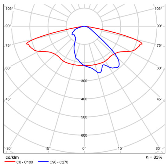
Figure 1.
Luminous intensity for SCHREDER TECEO GEN 2 2/5248/ 72LEDs 500 mA NW 740 109 W/457072.
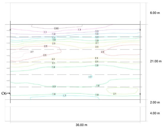
Figure 2.
Iso-luminance curves for main road—six lanes.
DIALux Evo does not have an option to move the observer to any desired position other than the center of the lanes. To overcome this limitation, an extra lane (virtual lane), was added to each side of the carriageway without changing the luminaires position. Consequently, the observer was positioned on the virtual lane, which in reality corresponded to the outside traffic area.
The proposed lighting arrangement that allows the placement of the observer outside the carriageway is represented in Figure 3. The average luminance was calculated in the same way for both observer positions, using the mean values obtained for the center of the six traffic lanes. In Figure 3, the areas considered for the average luminance calculation have been highlighted.
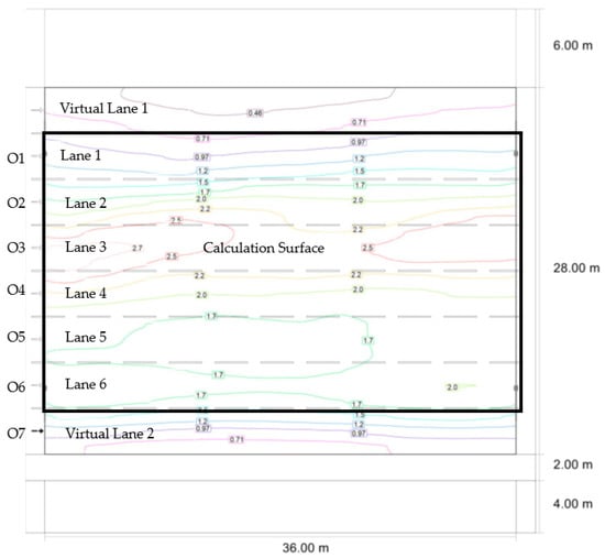
Figure 3.
Iso-luminance curves for main road—six lanes + two virtual lanes.
The values shown in Figure 2 and Figure 3 correspond to the luminance calculation for the opposite arrangement. The same calculation was repeated for staggered and single sided arrangements. A centralization of the results for each observer is shown in Table 2.
Table 2.
Average luminance comparison for a six-lanes carriageway with different observer positions.
Observers 1 to 6 (O1-O6), are positioned on the center of each lane in Figure 2, from top to bottom, while observer 7 is placed outside the carriageway on the virtual lane, as presented in Figure 3, which is the worst-case scenario for average luminance values.
The calculations were done for two particular situations:
- with the observer on lane 6, the position for which the program gives the average luminance of the entire road;
- with the observer O7 on the axis of the virtual lane 2, at 1.75 m from the edge of the calculation surface (Figure 3).
For a broader generality of the conclusions, all calculations were done for the R1–R4 type of asphalt and at 0°, 10°, 20° tilt angles.
To see whether the results are influenced by the road width, the previous calculation was repeated for a two-lanes carriageway. Figure 4 and Figure 5 present the street arrangement used for the second part of the study, with the observer O2 placed on the carriageway and O3 placed on the virtual lane, outside the carriageway (Figure 5).
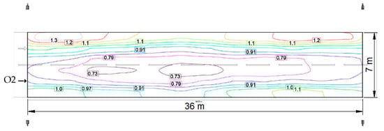
Figure 4.
Iso-luminance curves for main road—two lanes.
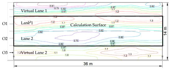
Figure 5.
Iso-luminance curves for main road—two lanes + two virtual lanes.
In the case of narrower roads, achieving the required design parameters required less powerful luminaires. Therefore, for the last two-lane lighting arrangement, the luminaire used was SCHREDER TECEO GEN 2 1/5244/ 24LEDs 500 mA NW 740 37.6 W/445172 [18], with the distribution curve presented in Figure 6.
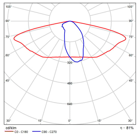
Figure 6.
Luminous intensity for SCHREDER TECEO GEN 2 1/5244/ 24LEDs 500 mA NW 740 37.6 W/445172.
The height of the luminaire for this calculation arrangement is 10 m. The distance from the center of the carriageway to the luminaire is 6.21 m and the asphalt type considered is R1–R4. The maintenance factor for all calculations is 1.
Table 3 presents the centralization of the results for a two-lanes road, with the observer placed on and outside the carriageway. By analyzing Table 2 and Table 3, one can see that, for opposite and staggered arrangements, the average luminance value is almost the same regardless of the tilt angle. The maximum error is just 4%, but in most cases, it does not exceed 2%. This difference between the two average luminance ratings has a significant impact on the measurement error when the observer is 1.75 m from the edge of the last lane. Since, for measuring the luminance with a digital camera, the equipment can be placed right next to the road, on the edge, the error can in fact be reduced.
Table 3.
Average luminance comparison for a two-lane carriageway with different observer positioning.
By contrast, for the single side lighting arrangement, the results are quite different. If we compare the values calculated with the observer outside of the carriageway with the minimum values of the average luminance, according to Table 3, it can be seen that the difference can be as high as 17% for the observers placed on the traffic lanes, which means that the relative error increased as the width of the carriageway became smaller. From the case study, it can be understood that the error increases when the road width is smaller. Even if we cut the distance in half, it would still result in an error of 8.5%. This error is unacceptable, given that the digital camera’s own errors are added to this type of measurement.
To test whether the average luminance for different observer positions is dependent on the distribution curve, the calculations have been repeated for the two-lanes carriageway (the worst case scenario) using two more luminaires, characterized by very different distribution curves, namely TECEO GEN2 1/5119/24 LEDs 500 mA NW 740 37.6 W/Back light/444962 [18], with the distribution curve represented in Figure 7, and TECEO GEN2 1/5249/24 LEDs 500 mA NW 740 37.6 W/445222 [18], with the distribution curve represented in Figure 8.
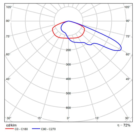
Figure 7.
Luminous intensity for SCHREDER TECEO GEN 2 1/5119/ 24LEDs 500 mA NW 740 37.6 W/444962.
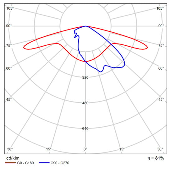
Figure 8.
Luminous intensity for SCHREDER TECEO GEN 2 1/5249/ 24LEDs 500 mA NW 740 37.6 W/445222.
Table 4 presents a centralization of the average luminance results for the last considered luminaires and with the observers positioned according to Figure 4 and Figure 5. In the case of the symmetric lighting arrangements, for the observer placed at 1.75 m from the edge of the last traffic lane, the maximum error was the same (2%) and was, as expected, less for the observer placed at the edge of the last traffic lane. In conclusion, regardless of the distribution curve of the luminaires, in the case of the symmetrical arrangement, the average luminance can be measured with sufficient accuracy by placing the equipment near the last traffic lane.
Table 4.
Comparison of the average luminance values for different distribution curves on a two-lanes carriageway.
3. Average Luminance Calculation for Road Lighting with Adjustable Observer Positioning
One limitation when using any street lighting design software is related to the observer’s position, which cannot be placed as desired. The observer is placed automatically by the software in the center of each traffic lane according to the European Standard [4] and, for the American Standard [10], in the center of an imaginary line parallel to the axes of the road that goes through the calculation. Because of this limitation, it is very difficult to study how the average luminance values vary if the observer is placed outside of the traffic area.
In order to avoid this problem, the authors have made a script that allows the calculation of the average luminance according to the European standards [4] with an adjustable position of the observer.
where:
- L—is the maintained luminance in candelas per square meter;
- k—is the index of current luminaire in the summation;
- nLU—is the number of luminaires involved in the calculation;
- Ik(C,γ)—is the luminous intensity in candela of the kth luminaire;
- fM—is the overall maintenance factor, depending on the light source lumen maintenance factor and luminaire maintenance factor;
- rk(tan ε, β)—is the reduced luminance coefficient for the current incident light path with angular coordinates (εk, βk);
- Hk—is the mounting height of kth luminaire above the surface of the road, in meters.
The calculation needs to select the luminous intensities, I(C,γ), for any calculation points. This means that the first step is to determine the angles C and γ for each calculation point. The method used, which was also presented in [16], is simpler than the one recommended by the standards.
In Figure 9, Q is the luminaire position, P is the calculation point, and QT the optical axis of the luminaire. If QT is perpendicular on the plan passing through PP′, and their intersection is the point V, then PV and P′V are perpendicular on the optical axis and form the angle φ. Angle C is determined based on angle φ. The value is translated in the quadrant, in which the calculation point is in reference to the luminaire. Because PP′V is a right triangle in P′, φ can be calculated with the formula:
where the segment length can be determined based on the coordinates of their ends:
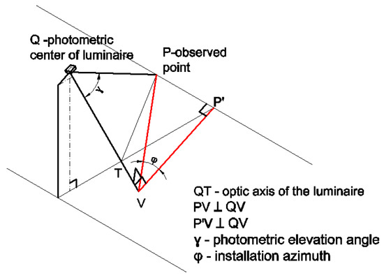
Figure 9.
Street and measurement points geometry, with P—calculation point.
Similarly, the angle γ can be determined from the right triangle PVQ (in V) using the formula:
The value of I(C,γ) for the calculated C and γ values specific to a certain calculation point is obtained by interpolation. For each luminaire, the I(C,γ) values can be found in the LDT file for some standard directions. These files can be read by several specialized softwares, the one used in this paper being LDT Editor. The luminous intensity I(C,γ) in the direction (C,γ) for a calculation point is determined by a linear interpolation between four values of luminous intensity, which corresponds to the closest directions compared with the calculation direction (C,γ).
The determination of the reduced luminance coefficient in the directions given by the angles β and ε, is shown in Figure 10. The reduced luminance coefficient table, also called the r-table, has been published by the CIE [19], but it can also be measured on site with specialized equipment [20,21,22].
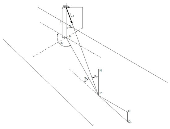
Figure 10.
Angular relationships for reduced luminance coefficient, considering luminaires at tilt during measurement, observer, and point of observation.
This type of measurement is not common practice, although the type of asphalt has a great impact on energy efficiency and lighting performance [23,24,25].
The program was first validated by comparing the calculation results in the standard observer position in the center of each traffic lane. The results were similar to the values calculated with DIALux Evo.
The use of the previously mentioned angles is usually considered difficult, and literature proposes some alternatives. The paper [26] has proposed a simplified method to directly take the luminance coefficient value based on the longitudinal and transverse distance from the luminaire to the calculation points. This method has a drawback though, as it neglects an important parameter: the observer’s position. The geometry used for the European standards is defined by the CIE [19,27] and is currently used with an observation angle of 1 ± 0.5° for a viewing distance between 60 and 160 m. The observer is positioned at 60 m from the calculation point, k1. For a 14 m width carriageway such as the one presented in this paper, the β angle can change with 10°, as demonstrated in Figure 11. After analyzing the r-table for the same ε, very different values of the reduced luminance coefficient can be observed. This suggests significant errors in the luminance calculation when the observer’s position is not taken into account.
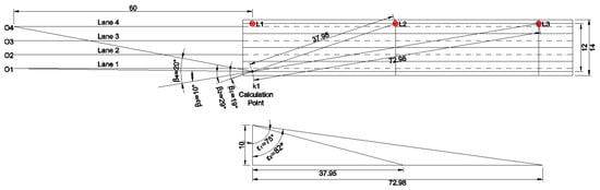
Figure 11.
Geometry for reduced luminance coefficient interpolation.
This idea was tested by comparing the values of the reduced luminance coefficient when considering observer 1 and observer 4 and the lamps L2 and L3, for one calculation point k1, as presented in Figure 11. The corresponding values from the R3 table [19] are centralized in Table 5.
Table 5.
Reduced luminance coefficient comparison for different observer positions viewing k1 calculation point.
Although the idea of simplifying the way of calculating the luminance by doing a luminance coefficient matrix based on longitudinal and transverse distances from luminaire to the calculation point is very good, the method should not exclude the position of the observer. A compromising solution can be the use of different tables for different transverse observer positions.
In the present study, the interpolation method recommended by the European Standard [4] has been used. Unlike I(C,γ), in order to determine the reflection factor of the asphalt, one must employ a quadric interpolation, for which nine values need to be taken into consideration instead of four [4].
Using Equation (1), the luminance values have been calculated for the observer positions O1, O2, and O3, represented in Figure 12, considering the three types of lighting arrangements opposite, staggered, and single sided, for a 0°, 10°, and 20° tilt.
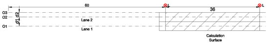
Figure 12.
Installation geometry for average luminance comparison with different observer positions.
The luminaire used for the calculation was SCHREDER TECEO GEN 2 1/5244/ 24LEDs 500 mA NW 740 37.6 W/445172 [18] with a maintenance factor of 1.
The results centralized in Table 6 are similar to the first case study done with DIALux Evo. For opposite and staggered lighting arrangements, the values are almost the same. The maximum error calculated is 1.3%, which, most likely, is due to the rounding of the values. Therefore, for these two types of lighting arrangements, the luminance can be measured on the exterior edge of the traffic lane near the lighting pole without any consequential errors.
Table 6.
Average luminance comparison for two-lanes carriageway with different observer positions.
For the single sided lighting arrangement, the situation is significantly different. The error reaches 7%, which is not acceptable. Therefore, for this lighting arrangement, a correction function must be found to determine the average luminance on the carriageway.
4. Determination of a Correction Function for Single Sided Lighting Arrangement
The average luminance for the single sided lighting arrangement changes depending on the observer’s position, as seen in Figure 13. The graphs are done for the geometries and positions of poles and luminaires as represented in Figure 3 and Figure 5. In Figure 13, the numbers of the center of the traffic lanes are represented on the abscissa. The observer O7 is placed outside the carriageway at 1.75 m on the side with the lighting poles.
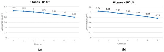
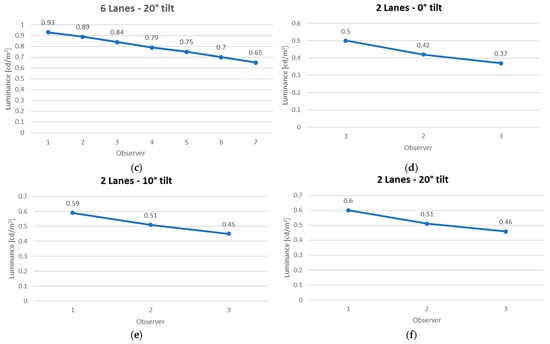
Figure 13.
Luminance evolution according to observer position: (a) Six-lanes carriageway and 0° tilt; (b) Six-lanes carriageway and 10° tilt; (c) Six-lanes carriageway and 20° tilt; (d) Two-lanes carriageway and 0° tilt; (e) Two-lanes carriageway and 10° tilt; (f) Two-lanes carriageway and 20° tilt.
The graphs show that luminance values have a very predictive evolution, in most cases being almost linear. At the taking over of the street lighting works, it is mandatory for the authorities to receive the detailed design project. This led to the idea to create a link between calculated and average luminance measurements, with a digital camera placed at the edge of the carriageway, as in the method described in [15]. By applying a correction function, the average luminance with the observer placed as per standard recommendation can be determined with much error reduction.
The geometry used for testing the correction function is presented in Figure 12. “In the transverse direction the observer shall be positioned in the centre of each lane in turn. Average luminance shall be calculated for the entire carriageway for each position of the observer. The operative value of average luminance shall be the lowest.” [4]. For the single sided lighting arrangement, the minimum average luminance value is, for the observer, positioned on the center of the first traffic lane, near the street lighting poles.
Observing the apparently linear evolution of the luminance from the graphs presented in Figure 13, the linear regression principle was first used in order to find the desired correction function.
The correction function must amend the luminance values measured at the edge of the carriageway. The first idea was to use a linear regression function to express the dependency between the luminance values and the observer’s position. If y represents the average luminance and x represents the observer’s position, then their linear dependence is:
where:
- k1—slope of the line.
The geometry of the installation is shown in Figure 12, and the values for observer 1 and 2 are centralized in Table 7.
Table 7.
Input data for linear regression function.
If O1 is considered the origin, the coordinate x becomes a distance and Equation (5) is:
where:
- Lav3—average luminance that needs to be calculated for O3;
- d—is the transverse distance from the first observer to the measurement point (equal to d1 + d2, see Figure 12).
Therefore, for the linear variation law, the average luminance for the observer placed in O3 can be calculated using the average luminance values for the observer placed in O1 and O2:
where:
- Lav1—average luminance calculated with the observer in the center of lane 1;
- Lav2—average luminance calculated with the observer in the center of lane 2;
- Lav3—average luminance calculated with the observer outside the carriageway as per Figure 12 geometry;
- d1—distance between the center of lane 1 and lane 2;
- d2—distance from the center of lane 2 to the observer at the edge of the carriageway (O3—position of digital camera).
Consequently, knowing Lav1 and Lav2 from the DIALux calculation, the measured value (with the observer placed on the center of lane two, as per Figure 12) of the average luminance can be approximated with:
where:
Table 8 is used to estimate the magnitude of the error in this approximation. It presents the difference between the average luminance calculated as per standard recommendation and the one calculated by applying Equation (8). In Equation (8), is the average luminance value calculated with the script developed in the previous section using different distances d2, and Lav3 is the average luminance value calculated with Equation (7).
Table 8.
Average luminance comparison between calculated values and proximate values based on the linear regression function.
Table 8 shows that the calculation error is 5% at 3 m distance from the axis of the lane near the poles and almost 24% at 7 m. This unacceptable error pushed the authors to find a better correction function.
Examining the variations in Figure 13, we looked for a better approximation than the linear one, respectively a law of variation in geometric progression. The average decrease in luminance for each meter of the observer’s movement (as an example, from O1 to O2 in Figure 12) is:
From the absolute value calculated with Equation (9), the relative value of the average luminance decreases compared with the reference value Lav1 and can be calculated as a relative loss coefficient (RLC) with:
Based on the geometric progression, one can assume that, for a 2 m movement, the relative loss is RLC2, and for a certain movement distance d2, the relative loss becomes RLCd2.
Therefore, the average luminance with the observer at the edge of the carriageway based on the values calculated from the last two traffic lanes is:
Consequently, to find the average luminance measured according to standards, one can use the average luminance measurement made outside the carriageway by applying the correction function RLC−d2, for example:
As previously observed, to estimate the magnitude of the error with this correction function, Table 9 presents a centralization of the results for observer O3 at different distances, d2, from the last traffic lane axes. The maintenance factor used is 1 and the tilt is 0°. There is almost no error for the first 2 m from the axis of the traffic lane and the magnitude of the error is very small for the next three meters. If the distance is bigger than 5 m, the error increases significantly, therefore this correction function method is useful when the observer is as close as possible to the traffic lane, on the side with the street lighting poles. However, almost no variation is observed in the first 3 m. This is more than enough for most streets, considering that in most cases the area outside of the traffic lanes is used either for parking, grass strip, or sidewalks, all of which are accessible to someone with a camera.
Table 9.
Average luminance comparison between calculated values and proximate values based on the geometric progression function.
The superiority of the second correction function is also highlighted by the graphical representation in Figure 14, in which the average luminance Lav2 is closer to the variation of the average luminance estimated with the correction function 2 (Lav2″) than that estimated with the correction function 1 (Lav2′).
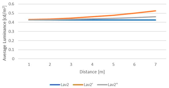
Figure 14.
Average luminance depending on the transverse distance from the observer O3 to the observer O2, as in Figure 12.
5. Errors in Luminance Measurements Done as Per 13201-4 Standard
The main conditions imposed by EN 13201 are the location and height of the observer, but also the equidistance of the points from which the luminance is measured.
Although fast measurement of the average value with a spot meter and a large measurement field is possible, standard 13201-4 states that: “As a less rigorous alternative, a luminance meter with a larger measurement cone can be used at a closer distance and a lower height. It is recommended that the measurement cone of the luminance meter should not exceed 30 min of arc, and the size of the measurement area on the road should not be greater than 0.5 m transversely and 2.5 m longitudinally” [5]. The minimum number of calculation points in the longitudinal direction is N = 10, and in the transverse direction is three for each traffic lane. This would mean that for a small two-lane road, the minimum number of calculation points is 10 × 6 = 60.
Due to the extended distance from the observer’s position to the calculation/measurement point, luminance-meters can have significant errors. Figure 15 presents how the surface measured (aimed) by the luminance-meter changes depending on the angle. If we take into consideration that the opening between poles is 40 m, the distance from the observer to the last calculation point is 98.5 m. Figure 15 presents the ellipse dimensions for this particular distance, considering three types of luminance-meters, with the most frequently used angles of observation: 0.1°, 1/3°, 1° [28]. Because of the very big dimensions of the 1° ellipse, this was not drawn at scale.
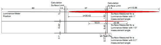
Figure 15.
Surface aimed on the asphalt at 98.5 m from the luminance-meter position for 0.1°, 1/3°, and 1° measuring angles.
Unlike lux-meters, the luminance-meter point measurement is actually a surface measurement at low angle on which the equipment measures the average value.
By analyzing Figure 15, one can see from the start that there is a big problem regarding the longitudinal dimension of the area measured. Even at low angles (0.1°), the ellipse longitudinal dimension is much larger than 3 m, the maximum distance between the calculation points recommended by the standards. The minimum longitudinal dimension of the ellipse for a luminance measurement positioned at 98.5 m from the calculation point is 10.9 m. This not only means that sections of the carriageway surface are taken into consideration multiple times, but also that the measurements at the beginning and at the end of the pole opening take into consideration surfaces outside the measured area, and, in some cases at the edge of the carriageway, it can even go outside of the project boundary, as seen in Figure 16.
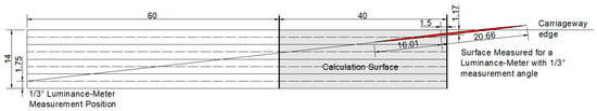
Figure 16.
Example of 1/3° luminance-meter measuring outside the project boundary.
Another very important error that appears when using this type of measurement equipment represents the fact that the ellipse projected on the asphalt is not symmetric to the measurement point position. For example, in Figure 15, one can see that for a 1° measurement angle, the length of the surface projected before the measurement point is 35.42 m, while the length after the calculation point is 115.98 m. This means that the average value in this point is totally compromised due to the fact that the surface after the measurement point represents 76.6 of the average value.
In order to understand how this error influences the results, Table 10 centralizes the values for all measuring angles, in absolute and relative values. The results show that even for a 1/3° luminance-meter, there can still be important differences between the surface considered before the measurement point and the one after it.
Table 10.
Comparison of the elliptical area before the calculation point with the area after the calculation point.
Unlike the luminance-meter, the imaging method is completely objective, ensuring traceability and repeatability in measurements. This method provides global qualitative information of the light environment. Not only is the imaging method much faster, it is much more accurate as well.
As in the case of the luminance-meter, the use of the imaging sensor raises some problems, as the photographic lens determines that for each pixel there is the same solid angle that receives the luminous flux reflected by the targeted asphalt. Transposing into a planar representation, Figure 17 indicates that, for equal viewing angles for each pixel, the horizontal plane surfaces are different. It follows that the average value calculated as an arithmetic average of the luminance values measured by the pixels is not perfect, as the average has the meaning as the average weighted by the asphalt surface targeted by each pixel (which is different). In order to verify this aspect, Figure 17 indicates, in principle, the geometry that establishes the connection between the pixel response and the image of the targeted asphalt.
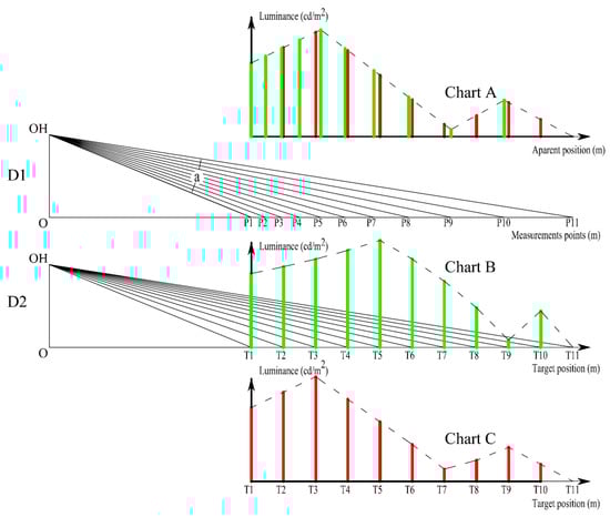
Figure 17.
How to determine the correction required to obtain the luminance measurement in the horizontal plane with equidistant steps according to EN 13201, using an imaging sensor with a constant viewing angle for each pixel (explanations are in the text).
In Figure 17, the OH observer is symbolized, positioned at a height of 1.5 m (O-OH segment) and a distance of 60 m from the first target point (O-P1 segment). The distances are not to scale, so that they can be visible. It is observed that there is a total viewing angle (a), which is evenly distributed for all pixels in the sensor. It turns out that the distances between the targeted points (respectively the size of the surfaces influencing the pixels) will be different, as the nearby asphalt target pixels provide more values per unit length compared to the distant asphalt target pixels (the P1–P2 segment is obviously smaller than P10–P11).
This aspect is illustrated in Figure 17, Chart A, where the luminance values measured by the pixels, relative to the points on the asphalt that were targeted, are illustrated in green (denser near the digital camera on the left of the chart). If this variation is represented graphically, with constant (and arbitrary) steps, we can obtain a variation similar to the one presented in Figure 17—Chart B. It is observed that there are several values measured on the left side of the graph, which influence the arithmetic mean and therefore the average luminance value. To determine which are the luminances in the equidistant points on the asphalt, the sketch from Figure 17—D2 was used, where the horizontal increment is constant, from T1 to T11.
The results are the angles for which the luminance is required to be read. However, as the imaging sensor provides us with luminance values for constant angular increments (Figure 17—D1), an interpolation operation is required. The graphical representation of this interpolation is indicated by the red segments in Figure 17—Chart A. After obtaining the values corresponding to the equidistant points on the field T1-T11, we can follow the result in Figure 17—Chart C. It is observed that the density of the measured values was enlarged to the right (in the distance) and decreased to the left (near the sensor). In this case, the arithmetic mean is lower, and this is the correction we are looking for.
An example of how the correction of the imaging sensor values work can be followed for an arbitrarily chosen longitudinal profile, presented in Figure 18.
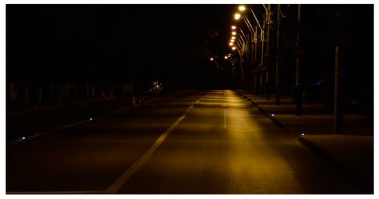
Figure 18.
The longitudinal direction of the profile for the luminance arbitrarily targeted to visualize the correction required for the values read by the optical sensor (white line in the center of the traffic lane).
The luminance values are read from bottom to top and the longitudinal profile of the luminances is available in Figure 19, illustrated in a blue color.
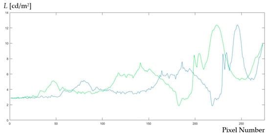
Figure 19.
Longitudinal luminance profile (cd/m2) referred to in Figure 18, values read on the ima-ging sensor with constant angular increment (blue) and corrected values for constant horizontal increment (green line), according to EN 13201.
In Figure 19, it is observed that the area with high luminance values on the right (at a bigger distance from the observer) expands, so that the average luminance value is higher. This fact is also confirmed numerically. The value of the uncorrected average luminance is 4.75 cd/m2, and the value of the corrected average luminance is 5.31 cd/m2. The very large difference justifies the need for this correction, especially for luminance distributions with a large non-uniformity factor and for single measurements.
After finding that the corrected average luminance decreased for the distribution in Figure 17 (with high luminance near the sensor) and increased for the distribution in Figure 19 (with high luminance for long-distance asphalt from the sensor), the question arises: What happens with this correction for distributions with relatively acceptable uniformity and with multiple measurements for the average luminance (according to EN 13201)?
This parameter is checked based on the imaging method. Figure 20 presents the night scene and directions by which the longitudinal profiles’ average luminance was calculated.
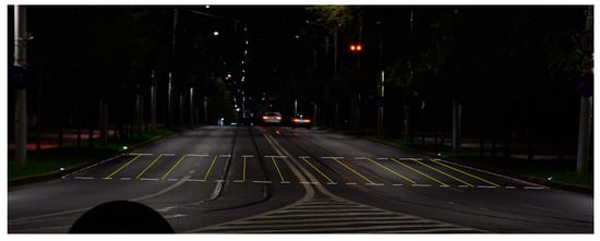
Figure 20.
Night scene with longitudinal profiles for the calculation of the average luminance according to EN 13201.
The values measured by the imaging sensor and the corrected values for constant horizontal increment, as well as the corrected error, are available in Table 11, the values being presented from left to right, corresponding to Figure 20.
Table 11.
Values read by the luminance-imaging sensor [cd/m2] with constant viewing angle and corrections for constant horizontal incremental steps.
The values confirm that corrections with different signs are obtained depending on the distribution of luminance. Overall, the gross and corrected values have a negligible difference of only 0.15%. The explanation is based on the relatively good luminance uniformity.
These types of determinations, in which the choice of points between which the longitudinal luminance is extracted and calculated, have a certain degree of subjectivity, but after repeated determinations, it was found that the differences remain negligible between successive calculations. As the overall calculation of the average values is much faster and more comprehensive, its usefulness is confirmed. The only precautionary measure is necessary in the case of lighting systems with a high degree of non-uniformity, where the correction of the imaging sensor for the constant incremental step, according to Figure 17, is necessary.
6. Average Luminance Measurements with Bias Observer Positioning
This section is dedicated to the validation of previous results which show that, in the case of symmetrical arrangements, the average luminance is approximately the same regardless of the position of the observer, inside or outside the carriageway. The validation was done through field measurements, performed on the Carol Boulevard, located in the city of Iasi, Romania.
Generally, the illuminance can be easily calculated, measured or evaluated. For the luminance calculation and measurement, the situation is totally different, as there are several variables to be taken into account.
The most unpredictable coefficient that influences the results is the asphalt reflection factor. There is equipment able to measure the asphalt reflection factor, and there are papers that suggest doing on-site measurements using this equipment, “on each road, providing a better representation of the road surface reflection properties and, consequently, more accurate luminance calculations of street and road lighting installations” [20]. However, for appropriate measurements, it is needed to stop traffic for a very long time. Moreover, there are some limitations to the angles for which the equipment can measure. Therefore, the use of the interpolation method cannot be excluded for now [29]. The photographic methods can be used to measure the reflectance properties of the asphalt [30], but this does not exclude the required stopping of traffic.
In case the measurements do not confirm the design hypothesis, measuring the reflection properties of asphalt becomes necessary.
There are some studies that have evaluated the average luminance with the observer at different distances. The influence of the angle of observation on the lighting criteria has been approached in [11]. The geometry associated with the study done in [11] is presented in Figure 21. Several problems can be identified. Firstly, the calculation surface is too narrow and the values are different due to the distance to the closest pole. Therefore, the average luminance calculation must be done for a full opening between two poles, similar to the specialized software calculations. Secondly (and most importantly), the study keeps the observer in a fixed position and evaluates average luminance for different surfaces at different angles of observation.
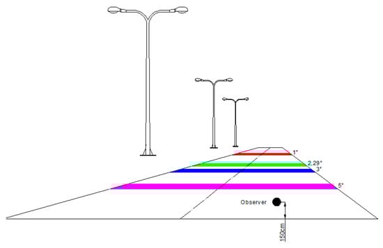
Figure 21.
Positioning of measurement area.
Using different surfaces to perform the calculation does not take into account the asphalt wear variability (as the same road wear can be very different depending on the location).
The case study presented in this section compares the average luminance value of the same calculation/measurement surface for different transverse observer positions.
The Nikon D5300 digital camera was used for this purpose. However, any digital camera can be used, even smart phones, if the manual operation mode is available and the calibration function is determined [31]. A simplified method for calibration is done by comparing the camera results with the ones from a precision luminance meter or even of a luminance standard [32]. In the present study, a calibration function determined in the laboratory with supplementary field correction for spectral sensitivity was used [33].
All average luminance measurements were done for the entire calculation surface from the axis centers of each traffic lane, as recommended by BS-EN 13201. In addition, two extra measurements were taken, placing the observer on the axis of each border of the carriageway. In Figure 22, the calculation surface is highlighted for each image. The area is represented by one pole opening. The installation’s geometry and observer positions are given in Figure 23.
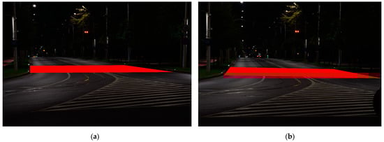
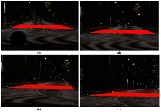
Figure 22.
Luminance images taken with the DSLR Camera for the same calculation surface highlighted in red, from different observer positioning: (a) Luminance image for observer 1—left border axis; (b) Luminance image for observer 2—axis of lane 1; (c) Luminance image for observer 3—axis of lane 2; (d) Luminance image for observer 4—axis of lane 3; (e) Luminance image for observer 5—axis of lane 4; (f) Luminance image for observer 6—right border axis.
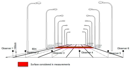
Figure 23.
Installation geometry for the series of images from Figure 22.
Figure 24 presents the luminance maps of the surface with the six viewing angles corresponding to the six observers, positioned as described in the illustration in Figure 23. The images reveal that spot luminance values can significantly differ with the observer’s position. This variation is not relevant for the average luminance value.
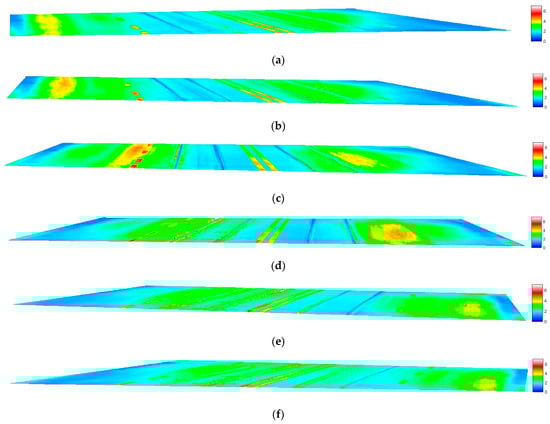
Figure 24.
Luminance map for observer 1—observer 6 position as per Figure 23: (a) Luminance map for observer 1—left border axis; (b) Luminance map for observer 2—axis of lane 1; (c) Luminance map for observer 3—axis of lane 2; (d) Luminance map for observer 4—axis of lane 3; (e) Luminance map for observer 5—axis of lane 4; (f) Luminance map for observer 6—right border axis.
A centralization of the average luminance values for the six luminance maps is given in Table 12. Values are very similar, and the maximum error is 6%. After analyzing the values on the luminance map, the conclusion is that most of the errors are due to the values on the road markups, not the asphalt itself. The important fact regarding the values is that the minimum value, as in the mathematical calculation, is at the edge of the carriageway. This means that the value measured at the boundary of the carriageway is almost identical to the minimum average luminance measured with the observer on the carriageway.
Table 12.
Average luminance comparison based on field measurements for observer 1–observer 6.
The numeric results confirm that, for symmetric arrangements, the average luminance value does not change considerably regardless of the observer’s transverse positioning. Outside the carriageway, the average luminance measurements should be done with the digital camera placed at the edge of the carriageway, as these results present minimum errors.
This somewhat surprising result deserves a deeper analysis. As a first observation, in the case of the opposite lighting arrangement, for a certain calculation point, the sum of the two β angles corresponding to the opposite luminaires is always constant. Moving the observer at the edge of the carriageway, the deviation angle β increases for one pole and decreases for the other pole by the same amount. As a consequence, the reduced luminance coefficient values corresponding to the two poles vary in the same opposing manner, and compensate each other, more or less, depending on the influence of the ε angle.
From the two parameters of the reduced luminance coefficient table (r-table), the only variable changing with the observer position is the deviation angle β. Figure 25 gives the geometry that helps in the analysis of β variation. For the surface calculation defined by standards, placed at 60 m from the observer, and moving the observer from O4 (the center of the lane with the lowest average luminance) to O5 at the edge of the road, the largest variation of β is recorded for the calculation point located next to the L4 pole. For that point, Δβ = 1.6708°, for any other calculation point the β-variation is smaller.
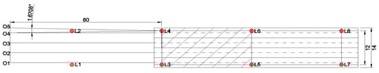
Figure 25.
Geometry for assessing the variation of the deviation angle β.
Looking in the r-table, for β bigger than 75°, it is a low variation with β for the reduced luminance coefficient values. Therefore, moving the observer at the edge of the road and producing a variation of β with a maximum of 1.6708° results in almost no difference for the reduced luminance coefficient values. This means that, when measuring the luminance from the road edge, the contribution to the luminance of the luminaires L1–L4, placed before the calculation surface, is not influenced significantly by the change of β.
The r-table analysis also shows that the values of the ε angle are important. For tgε > 10, the R-values are small, regardless of β values. Therefore, moving the observer position to the edge of the road, produces significant changes only in the luminance produced by the luminaires L5, L6, L7, and L8.
7. Confirmation of Correction Function through Luminance Measurements with an Imaging Sensor
This section is dedicated to the validation of previous results from Section 4 that proposed a correction function for a single sided lighting arrangement in order to measure the average luminance value with an imaging sensor positioned at the edge of the carriageway, near the lighting pole. The validation was done by field measurements, performed on Fagului street, located in the city of Iasi, Romania.
Figure 26 presents the geometry of the installation and Figure 27 presents the luminance map for observer O1–O4.
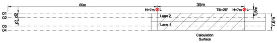
Figure 26.
Fagului street installation geometry.
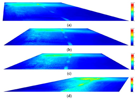
Figure 27.
Luminance map for observer 1—observer 4 position as per Figure 26 installation geometry: (a) Luminance map for observer 1—left border axis; (b) Luminance map for observer 2—axis of lane 1; (c) Luminance map for observer 3—axis of lane 2; (d) Luminance map for observer 4—right border axis.
As Section 4 suggests, in theory, one should be able to calculate the average luminance value for observer 2 based on the observer 1 value and the values from the design calculation.
In order to confirm this hypothesis, we first did the DIALux Evo calculation. Considering that the installation is old, the maintenance factor of the luminaire was considered 0.67.
As the previous study has shown, the minimum average luminance value is for the observer O1, near the lighting pole.
A centralization of the average luminance measured for the luminance map in Figure 27 and for the DIALux Evo calculations are given in Table 13. Considering that we only need the values calculated with the observer in the center of each traffic lane, the average luminance was calculated only for the O2 and O3 positions. The luminaire used in the calculation was a Philips SGS453 C GB 1xSON-TPP150W.
Table 13.
Average luminance comparison based on field measurements for observer 1–observer 4.
As expected, due to the usage of the luminaire and asphalt, the results were not exactly the same, but the question is: How much this influences the correction factor? By applying Equation (12) to the value measured from the O1 position, based on the DIALux Evo-calculated average luminance, one can calculate the measured value when the digital camera is positioned in the center of lane 2.
Considering that both the asphalt reduced luminance coefficient and luminaire usage are not exactly known, an error of 4.1% is more than reasonable. This is why measuring the average luminance value from the edge of the carriageway is suitable even for a single sided arrangement if the correction function is applied.
8. Conclusions
This paper proves that average luminance measurements with a digital camera can be done with the observer positioned at the edge of the carriageway with negligible errors for symmetric lighting arrangements. This particular parameter has an important role in evaluating the efficiency of a street lighting installation. Therefore, in order to achieve a sustainable system, average luminance measurements on traffic lanes are mandatory.
For single sided arrangements, the paper proposes a new correction function, which can be used to calculate the average luminance value with the observer on the carriageway, based on measurements taken by the camera positioned outside of the traffic area, at the edge.
The paper also calculates the errors in luminance measurements done as per 13201-4 standard recommendations, with different angles of measurement luminance-meters. The conclusions are that wide angle luminance-meters are not at all to be recommended, even at small distances from the calculation point, due to the big differences between the area taken into consideration before the calculation point and the area after it. Even at low measurement angles, the error is still significant due to the large dimension in longitudinal direction.
In the same section there is an assessment of an imaging sensor which has for each pixel the same solid angle that receives the luminous flux, reflected by the targeted image, and analyzes how this fact influences average luminance measurements. Transposing into a planar representation, for equal viewing angles for each pixel, the horizontal plane surfaces are different. This means that the average value calculated as an arithmetic average of the luminance values measured by the pixels will not be accurate. This occurs because the average has the meaning of an average weighted by the asphalt surface targeted by each pixel (which is different).
Based on the case study, the values confirm that corrections with different signs are obtained depending on the distribution of luminance. Overall, the gross and corrected values have a negligible difference of only 0.15%. This confirms that the measurement of average luminance with an imaging sensor is the most reliable method, with minimum error.
The only precautionary measure should be taken for a high degree of non-uniformity of luminance, where, in this paper, we proposed a correction of the imaging sensor for the constant incremental step.
Considering that, in most cases, the average luminance is the most important parameter to check when doing any examinations of works, the possibility of measuring this value with the digital camera placed outside the traffic area, with minimum, or even no error, is a very important step in street lighting measurements.
Author Contributions
Conceptualization, A.V.R.; methodology, A.V.R., C.D.G. and D.D.L.; software, A.V.R.; validation, C.D.G. and D.D.L.; formal analysis, D.D.L. and G.L.; investigation, C.D.G. and A.V.R.; resources, C.D.G. and A.V.R.; data curation, A.V.R., C.D.G. and D.D.L.; writing—original draft preparation, A.V.R.; writing—review and editing, D.D.L., C.D.G. and G.L. All authors have read and agreed to the published version of the manuscript.
Funding
This work was supported by a publications grant of the TUIASI, project number GI/P25/2021.
Institutional Review Board Statement
Not applicable.
Informed Consent Statement
Not applicable.
Data Availability Statement
The data are available from the corresponding author upon request.
Conflicts of Interest
The authors declare no conflict of interest.
References
- Commission Internationale de l’Éclairage (CIE). Calculation and Measurement of Luminance and Illuminance in Road Lighting, CIE 030:1976; Commision Internanionale de l’Eclairage: Vienna, Austria, 1976; ISBN 978-9-290340-30-0. [Google Scholar]
- European Standard, Road Lighting—Part 1: Guidelines on Selection of Lighting Classes (EN 13201-1:2014); CEN: Brussels, Belgium, 2015.
- European Standard, Road Lighting—Part 2: Performance Requirements (EN 13201-2:2015); CEN: Brussels, Belgium, 2015.
- European Standard, Road Lighting—Part 3: Calculation of Performance (EN 13201-3:2015); CEN: Brussels, Belgium, 2015.
- European Standard, Road Lighting—Part 4: Road Lighting Methods of Measuring Performance (EN 13201-4:2015); CEN: Brussels, Belgium, 2015.
- European Standard, Road Lighting—Part 5: Energy Performance Indicators (EN 13201-5:2015); CEN: Brussels, Belgium, 2015.
- Available online: https://www.dialux.com/en-GB/download (accessed on 5 April 2021).
- Available online: https://www.lightingreality.com/ (accessed on 6 April 2021).
- Available online: https://reluxnet.relux.com/en/downloads.html (accessed on 6 April 2021).
- Illuminating Engineering Society of North America (IESNA). ANSI/IES Recommended Practice for Roadway Lighting No. RP-8-18; Illuminating Engineering Society of North America, Roadway Lighting Committee, ANSI/IES: New York, NY, USA, 2018. [Google Scholar]
- Muzet, V.; Bernasconi, J.; Iacomussi, P.; Liandrat, S.; Greffier, F.; Blattner, P.; Reber, J.; Lindgren, J. Review of Road Surface Photometry Methods and Devices—Proposal for new Measurement Geometries. Light. Res. Technol. 2020, 53, 213–229. [Google Scholar] [CrossRef]
- Commission Internationale de l’Éclairage (CIE). Recommended System for Visual Performance Based Mesopic Photometry, CIE 191:2010; Commision Internanionale de l’Eclairage: Vienna, Austria, 2010; ISBN 978-3-901906-88-6. [Google Scholar]
- Uchida, T.; Ayama, M.; Akashi, Y.; Hara, N.; Kitano, T.; Kodaira, Y.; Sakai, K. Adaptation Luminance Simulation for CIE Mesopic Photometry System Implementation. Light. Res. Technol. 2016, 48, 14–25. [Google Scholar] [CrossRef] [Green Version]
- Greffier, F.; Muzet, V.; Boucher, V.; Fournela, F.; Dronneau, R. Use of an Imaging Luminance Measuring Device to Evaluate Road Lighting Performance at Different Angles of Observation, Commision Internationale de l’Eclairage. In Proceedings of the 29th CIE Session, Washington, DC, USA, 14–22 June 2019; pp. 553–562. [Google Scholar] [CrossRef]
- Rusu, A.V.; Galatanu, C.D.; Lucache, D.D. Luminance Uniformity Analysis Based on Digital Camera Measurements. In Proceedings of the 11th International Conference and Exposition on Electrical And Power Engineering (EPE), Iasi, Romania, 22–23 October 2020; pp. 392–396. [Google Scholar] [CrossRef]
- Rusu, A.V.; Galatanu, C.D.; Lucache, D.D. Field Measurements for Street Lighting Assessment. In Proceedings of the 11th International Conference and Exposition on Electrical And Power Engineering (EPE), Iasi, Romania, 22–23 October 2020; pp. 668–673. [Google Scholar] [CrossRef]
- Lipnický, L.; Gašparovský, D.; Dubnička, R. Influence of the Calculation Grid Density to the Selected Photometric Parameters for Road Lighting. In Proceedings of the Lighting Conference of the Visegrad Countries (Lumen V4), Karpacz, Poland, 13–16 September 2016. [Google Scholar] [CrossRef]
- Available online: https://www.schreder.com/en/products/teceo-led-street-lighting (accessed on 1 March 2021).
- Commission Internationale de l’Éclairage (CIE). Road Surface and Lighting, CIE 66:1984; Commision Internanionale de l’Eclairage: Vienna, Austria, 1984; ISBN 978-3-901906-72-5. [Google Scholar]
- Strbac-Hadzibegovic, N.; Strbac-Savic, S.; Kostic, M. A New Procedure for Determining the Road Surface Reduced Luminance Coefficient Table by On-site Measurements. Light. Res. Technol. 2017, 51, 65–81. [Google Scholar] [CrossRef]
- Laurent, M. Characterisation of Road Surfaces Using Memphis Mobile Gonioreflectometer. In Proceedings of the International CIE Symposium on Road Surface Photometric Characteristics, Torino, Italy, 25–26 May 2008. [Google Scholar]
- Jackett, M.J.; Frith, W.J. Measurement of the Reflection Properties of Road Surfaces to Improve the Safety and Sustainability of Road Lighting, NZ Transport Agency Research Report 383; NZ Transport Agency: Wellington, New Zealand, 2009.
- Fotios, S.; Boyce, P.; Ellis, C. The Effect of Pavement Material on Road Lighting Performance. Lighit. J. 2006, 71, 35. [Google Scholar]
- Ekrias, A.; Ylinen, A.; Eloholma, M.; Halonen, M. Effects of Pavement Lightness and Colour on Road Lighting Performance. In Proceedings of the CIE International Symposium on Road Surface Photometric Characteristics: Measurement Systems and Results, Torino, Italy, 25–26 May 2008. [Google Scholar]
- Gidlung, H.; Lindgren, M.; Muzet, V.; Rossi, G.; Iacomussi, P. Road Surface Photometric Characterisation and Its Impact on Energy Savings. Coatings 2019, 9, 286. [Google Scholar] [CrossRef] [Green Version]
- Zhou, S.; Chen, C.; Han, H. A New Method of Calculating the Luminance Distribution in Straight Road Lighting; China International Forum on Solid State Lighting (SSLCHINA): Guangzhou, China, 2014; pp. 32–34. ISBN 978-1-4799-6697-4. [Google Scholar]
- Commission Internationale de l’Éclairage (CIE). Road Lighting Calculations, 2nd ed.; CIE 140:2019; Commision Internanionale de l’Eclairage: Vienna, Austria, 2019; ISBN 978-3-902842-56-5. [Google Scholar]
- Available online: https://www5.konicaminolta.eu/ru/measuring-instruments/products/light-display-measurement.html (accessed on 7 April 2021).
- Debergh, N.; Embrechts, J.J. Mathematical Modelling of Reduced Luminance Coefficients for Dry Road Surfaces. Light. Res. Technol. 2008, 40, 243–256. [Google Scholar] [CrossRef]
- Galatanu, C.D.; Canale, L. Measurement of Reflectance Properties of Asphalt using Photographical Methods. In Proceedings of the International Conference on Environment and Electrical Engineering and 2020 IEEE Industrial and Commercial Power Systems Europe (EEEIC/I&CPS Europe), Madrid, Spain, 9–12 June 2020; ISBN 978-1-7281-7455-6. [Google Scholar]
- Jin, J.; Lee, S.; Byun, Y. Mobile-based Luminance Measurement for Night Scene. In Proceedings of the International Conference on Computer Application Technologies, Matsue, Japan, 31 August–2 September 2015; p. 148. [Google Scholar] [CrossRef]
- Gbologah, E.F.; Guin, A.; Purcell, R.; Rodgers, M. Calibration of a Digital Camera for Rapid Auditing of In Situ Intersection Illumination. Transp. Res. Rec. J. Transp. Res. Board 2017, 2617, 35–43. [Google Scholar] [CrossRef]
- Galatanu, C.D. Luminance Measurements for Light Pollution Assessment. In Proceedings of the International Conference on Electromechanical and Power Systems (SIELMEN), Iaşi, Romania, 11–13 October 2017; pp. 456–461. [Google Scholar] [CrossRef]
Publisher’s Note: MDPI stays neutral with regard to jurisdictional claims in published maps and institutional affiliations. |
© 2021 by the authors. Licensee MDPI, Basel, Switzerland. This article is an open access article distributed under the terms and conditions of the Creative Commons Attribution (CC BY) license (https://creativecommons.org/licenses/by/4.0/).