Abstract
Carbon emissions (CE) reduction has been an important measure to control global warming. With the deepening of internationalization, the import and export trade can have a significant influence on CE. In this study, the panel data of 282 cities in China from 2003 to 2016 were employed, and linear regression analysis with fixed effects, feasible generalized least squares and Driscoll–Kraay estimators were performed to assess the separate impacts of import and export trade on CE. The results show that there is a positive correlation between imports and CE, while the relationship is contrary for exports. The panel threshold regression method was further used for regression, and it found that there was one threshold value for gross domestic product (GDP) and two threshold values for gross industrial output (GIO) in the model. According to the division of threshold value, the impact of import trade on CE will turn from positive to negative, while the impact of export trade on reducing CE will be further enhanced. The structure of China’s import and export trade are used to illustrate the underlying mechanism of the different effects. For controlling CE in international trade, China should import more high-tech products to upgrade high-emission industries, and reduce the proportion of labor-intensive products exported.
1. Introduction
Over the past 10 years (2010–2019), China’s fossil carbon dioxide emissions (CE) have grown at an annual growth rate of 1.2%, dominating the global growth trend [1]. China pledged in the Paris Accord that its CE would peak by around 2030 [2]. The government has introduced measures in various aspects to reduce CE and curb global warming. Therefore, the analysis of the influencing factors of CE and the corresponding mechanisms can help policy makers to better adjust energy strategies and formulate carbon reduction policies.
Since China’s accession to the World Trade Organization (WTO), the volume of its imports and exports is increasing year by year. Some literature showed that international trade will increase China’s CE [3,4,5]. On the other hand, environment-friendly technologies from developed countries can flow into China to reduce CE [5,6]. Furthermore, imports and exports in international trade have different influences on CE. Exports have been shown to contribute more to China’s CE than imports [7,8]. For the 20 Asian countries, exports will lower consumption-based CE, whereas imports increase it [9]. Similar results can be found in other studies [10]. In other words, imports and exports have asymmetric and heterogeneous effects, but they are rarely regarded as separate variables in empirical analysis. Thus, the systematic assessment of impacts of imports and exports is of great significance for CE reduction.
Moreover, existing studies of CE in China are mostly focused on the provincial level [11,12,13]. In fact, due to different geographical locations, economic foundations and industrial structures, the trade contribution of each city varies greatly. For instance, in a recent study by Mi et al. [14] of 11 cities in China, they found that six of the cities are dependent on imports for their CE, but the other five are the opposite. Against such backgrounds, it is necessary to analyze this issue from the city level.
In this study, we calculated the CE of 282 Chinese cities from 2003 to 2016, and these data were used for regression analysis. On this basis, the panel threshold model can help to explore the relationship between imports and exports and CE in a nonlinear framework. The rest of the paper is structured as follows. Section 2 provides the literature review of CE and international trade. The estimated model and data management are described in Section 3. The empirical results of linear analysis and panel threshold analysis and their corresponding mechanism are discussed in Section 4. The conclusion and policy implications are presented in Section 5.
2. Literature Review
In the following, the literature review is conducted from the perspective of the international trade–CE nexus.
Trade openness is often used to represent the level of international trade, which is defined as trade value as a percentage of gross domestic product (GDP) [15]. Using cointegration techniques, Chebbi et al. [16] found that trade openness could exacerbate the greenhouse effect in the short and long term. Fang et al. [17] and Mahmood et al. [18] have also obtained a consistent conclusion. However, for the 35 Organization for Economic Cooperation and Development (OECD) countries, trade openness has a negative impact on CE [19]. As for China, Ang [20] found that greater trade openness tends to cause more CE in China via the corresponding data from 1953 to 2006. According to the research results of Qi et al. [21], there is an “inverted U” relationship between trade openness and CE; that is to say, CE may also decrease with the increase of trade level. In general, scholars have not reached a consensus on the relationship between trade openness and CE.
The trade openness will bring in financial support, leading to economic expansion and factory production, which can significantly increase CE. Thus, some researchers have studied the impact of foreign direct investment (FDI) on domestic CE. Li et al. [22] used extended STIRPAT model, and a positive effect of FDI on the CE was found. In a study by Yang et al. [13], FDI increased the CE of China’s provincial industries between 1999 and 2011. On the other hand, foreign products can motivate local improvement or invention of more technological products. These kinds of technology spillover effects are beneficial in reducing CE. By using provincial data sets in China from 1995 to 2011, Wang et al. [23] observed an insignificant but positive effect of FDI on the reduction of CE. Huang et al. [24] also found that FDI decreased the provincial CE in China from 2000 to 2013.
In view of the complex influences of international trade on CE, the role of imports and exports are examined separately in some studies. In order to investigate the impacts of international trade on CE in China–Japan–ROK FTA countries, Dou et al. [25] selected panel datasets from 1970 to 2019 for empirical analysis and divided the total trade into imports and exports. They concluded that imports can lead to an increase in CE, while exports significantly reduce a country’s CE. Using the data from the BRICS countries for the period 1990–2017, the same results can be obtained [26]. This is because more imports will result in more domestic consumption-based CE, while more exports mean fewer goods and services consumed domestically. These similar conclusions are also valid in the G7 countries [27], OECD and non-OECD countries [28] and Mexico, Indonesia, Nigeria and Turkey (MINT nations) [29]. Besides, it was found by Shahbaz et al. [30] that export diversification is beneficial to energy conservation, from which we can infer that exports are beneficial to the reduction of CE. These findings are different from some other conclusions. For example, Ahmed et al. [31] employed the annual panel data from eight developing countries between 1980 and 2014, and the study showed that exports are a significant factor in CE. The CE embodied in China’s international trade from 1997 to 2007 was estimated in another study [32], and the researchers found about 10.03–26.54% of China’s CE was generated in the export manufacturing process, while the imports only accounted for 4.40–9.05% CE. Therefore, the impacts of imports and exports may be complicated in different regions and over different time periods. To make more targeted policy recommendations, it is important to discuss these impacts on CE after China’s accession to the WTO from the urban level.
3. Methodology
3.1. Estimated Model
When studying the issue of CE, GDP is an indispensable influencing factor [10,26,31,33,34,35], and it is generally positively correlated with CE. In addition, the regions with higher population densities [35], population size [36] and higher level of population urbanization [33] can have higher CE. In some regions, the effect of population may not be significant [34]. As for industrial development, the proportion of high energy-consumption sector CE to total industrial emissions is steadily increasing in China [36], and the adjustment of industrial structure is an effective way to reduce CE [37]. With the development of technology, the application of green energy technology can effectively reduce emissions [38]. In the selected G20 countries, innovation has also been proven to have a negative relationship with CE [39].
Based on previous studies, the following control variables at the city level were selected in this study: the gross domestic product (GDP), the natural growth rate of population (POP), the gross industrial output (GIO), the number of technology practitioners (TEP) and the ventilation coefficient (VC). The first four variables cover the cities’ economy, population, industry and technology development. The ventilation coefficient (VC) is a commonly used instrumental variable in environmental economics, and its detailed calculation is introduced in Section 3.2. Thus, the following model is proposed,
where the subscript i represents cities, the subscript t represents years, and IMP and EXP denote total imports and total exports, respectively. The “ln” in Equation (1) indicates the natural logarithm, and the indicates the random disturbance. These coefficients (m = 0, 1, 2, …, 7) are to be estimated.
3.2. Data Management
The relevant data of 282 cities in China from 2003 to 2016 were selected for empirical analysis in this paper. This basically covers the Chinese cities for which the data can be found, as detailed in the Supplementary Materials. Table 1 shows the basic description of these data. According to the China City Statistical Yearbook and the public data, the total imports and exports (IMP and EXP) can be obtained. The data of GDP, POP, GIO and TEP can be found in the China City Statistical Yearbook, as well. It is worth noting that the GDP used is deflated by the deflator, with 2003 as the base year. As for the CE and VC, they need to be calculated as follows.

Table 1.
Description of variables.
The CE were calculated according to the IPCC guidelines [40], based on energy data from individual cities. This calculation method has been successfully applied by Huang et al. [41] and the calculation equation is as follows,
where Ei denotes the energy consumptions for energy i, and NCV, CEF and COF are the low calorific value, carbon content and the rate of carbon oxidation, respectively. According to the China Energy Statistical Yearbook, China City Statistical Yearbook, etc., the seven most important energy sources calculated are raw coal, gasoline, kerosene, diesel oil, fuel oil, liquefied petroleum gas and natural gas, respectively.
The ventilation coefficient (VC) is calculated according to Equation [42],
where WS denotes the wind speed at 10 m height, and BLH denotes the atmospheric boundary layer height. These data were obtained from the European Centre for Medium-Term Weather Forecasting (ECMWF).
4. Results and Discussions
4.1. Panel Unit Root Tests
In order to avoid a possible spurious regression, the unit root tests for each variable should be conducted before regression. In this paper, the LLC method proposed by Levin, Lin and Chu [43] and the IPS method proposed by Im, Pesaran and Shin [44] were used to jointly verify the stationarity of variables. The corresponding results are shown in Table 2, and the null hypothesis of unit roots was rejected within the 1% significance level. Therefore, all the variables were stationary, which is the premise of the following panel regression.
Table 2.
Results of panel unit root tests.
4.2. Linear Regression Analysis
To determine whether the fixed effect (FE) or random effect (RE) was more appropriate for this model, the Hausman test was performed. Table 3 shows the relevant calculation results. The null hypothesis was rejected at the significance level of 1%, which indicates that the FE should be used for regression. After employing the modified Wald test for heteroskedasticity [45] and Wooldridge test for autocorrelation [46] in the FE regression model, however, the result may be biased due to the heteroskedasticity and serial correlation. In response to this possible problem, the feasible generalized least squares (FGLS) and Driscoll–Kraay (DK) estimators [47] were used. The corresponding empirical results are also presented in Table 3 for comparison.
Table 3.
Results based on linear panel regression analysis.
As shown in Table 3, imports (lnIMP) had a positive effect on CE, while exports (lnEXP) had a negative effect, at a very significant level. Their corresponding coefficients were 0.0056 and −0.0151, respectively, although the results in the FGLS method were slightly different. Some related studies have also shown the similar results [25,26,27,28,29]. Tang et al. [48] believe that the trend of China’s CE exports embodied has been gradually changed due to the improvement of the industrial and energy consumption structure. For our research results, it can be concluded that the further restructuring of China’s trade structure has been effective in curbing CE in recent years, since the study period was from 2003 to 2016.
Of all the variables, urban economic development (lnGDP) has a very significant impact; namely, 1% economic growth leads to an approximately 0.7% increase in CE at the 1% significance level. It is obvious that industrial development (lnGIO) will also increase CE, because energy consumption is closely linked to industrial development. As for the natural growth rate of population (POP), the POP has a negative correlation with CE, which may be different from our conventional understanding, but similar results have also been reported [49,50]. Although the energy consumption increases with population growth, it may stop increasing when there is a surplus of labor. Besides, the aging of the population will also reduce the labor force, affecting economic development. Therefore, when the positive effect of POP on CE is less than the negative effect, this negative correlation occurs.
Technology development (lnTEP) was also considered in our estimates. Obviously, it is negatively correlated with CE although the three estimated coefficients are not exactly the same. The larger the value of air ventilation coefficient (lnVC) is, the stronger the air flow is, so it should be negatively correlated with CE. However, its corresponding coefficients are positive in Table 3. So, this linear analysis may not fully show its effects as the coefficients in the FE and DK estimators are quite small, at a non-significant level.
4.3. Panel Threshold Regression Analysis
The impact of international trade on CE may differ from region to region. For instance, a different urban population density [21], regional intellectual property protection level [51] and urbanization level [52] can lead to the different effects of trade on CE. The economic development levels of the 282 cities in our study are quite different, so the results obtained by linear regression may not fully reflect the relationship between international trade and CE. In view of this, the panel threshold regression model proposed by Hansen [53,54] should be employed. The threshold variable can divide the sample into several sub-samples and calculate regression for each sub-sample respectively, so that different effects can be obtained within the range of different threshold variables. If there is a single threshold, the model is written as,
where X is a set of explanatory variables, q is a set of threshold variables, is the calculated threshold value, denotes the fixed effects, denotes a zero mean, finite variance, i.i.d. disturbance, and θ and β are the corresponding coefficients. To be specific, when the threshold variable q is lower than the threshold value γ, the coefficients are θ1 and β1, and otherwise they are θ2 and β2.
If there exists a single threshold, whether there are double thresholds needs to be determined next. The model with two thresholds is as follows,
where and are the two corresponding thresholds, respectively, and θm and βm (m = 1, 2, 3) are the corresponding coefficients.
In our models, one of the main differences among cities was the level of economic development (lnGDP), which is also a variable highly correlated with CE. In addition, the level of industrial development in a region (lnGIO) is a more direct reflection of the region’s CE. Therefore, the variables lnGDP and lnGIO were selected as threshold variables in the following regressions.
First of all, the possible numbers and value of threshold were tested with the threshold variables selected as lnGDP and lnGIO, respectively. The null hypothesis was that the threshold does not exist. Through the calculation of F-statistics, there will be at least one threshold if the hypothesis is rejected. Then the double threshold test will be done, and so on. The results of the threshold tests are shown in Table 4. It can be seen that a single threshold existed at 1% significance level when lnGDP was chosen as the threshold variable, and the corresponding lnGDP was 17.76. When the threshold variable shifted to lnGIO, the two threshold values were 16.41 and 18.10 at 1% significance level, respectively. In general, the nexus of CE and imports and exports was nonlinear, which was sensitive to the lnGDP and lnGIO changes.
Table 4.
Threshold tests for imports and exports.
Based on the threshold tests, the corresponding estimated coefficients are presented in Table 5 when lnGDP and lnGIO are at different levels. These significant coefficients have validated our model. It is worth noting that the coefficient before lnVC is always negative in this table, which is different from linear regression. It also shows that this nonlinear relationship is more in line with the actual situation.
Table 5.
Results based on nonlinear panel threshold regression analysis.
The first eight rows in Table 5 show the estimated coefficients of all the variables with lnGDP as the threshold variable and lnIMP as an independent variable. It can be seen that these coefficients are significant at the 1% level. When the lnGDP is smaller than 17.76, the coefficient of lnIMP is 0.0052, otherwise it is −0.0087. This indicates that imports can be negatively correlated with CE only when the economic level further develops. As shown in rows nine to sixteen, a similar trend exists when lnGIO is the threshold. Moreover, the negative correlation is more pronounced with lnGIO larger than 18.10, because the coefficient has shifted to −0.0155. Thus, from the perspective of imports, international trade can increase CE for underdeveloped cities, while it can effectively reduce CE for developed cities.
As for exports (lnEXP), rows 17 to 32 of Table 5 indicate that all the coefficients in models are also basically significant at the level of 1%, and the relationship between lnEXP and CE is always negative. However, this effect is always nonlinear. When lnGDP is less 17.76, the coefficient of lnEXP is −0.0145, and it will be −0.0277 when lnGDP is greater than 17.76. In other words, the more developed the economy, the more effective exports can be in inhibiting CE. When there exist three thresholds, namely with lnGIO as the threshold value, the coefficient changes from −0.0137 to −0.0228 and −0.0336, as shown in row 26. In general, a more developed economy or industry can be more significant in reducing CE though exports always have a negative relationship with CE.
4.4. Mechanism Analysis
According to the above linear regression and panel threshold regression analyses, urban exports have a negative impact on CE, while imports may increase or decrease CE. To explore the mechanism, we will try to illustrate this in terms of the structure of international trade. Figure 1 shows the proportionate change of primary and manufactured products in import and export trade in China from 2001 to 2019. It can be seen from Figure 1a that the share of imported manufactured products declined significantly, while the share of imported primary products increased from less than 20% in 2001 to 35% in 2019. In fact, the proportion of fossil fuels and related raw materials in imported primary products was basically maintained at more than 40%. Thus, the increase of imported primary products is bound to lead to an increase in CE from industrial production. As for exports, the proportions of these two categories were basically unchanged, although there was a slight increase in manufactured products and a slight decrease in primary products, as shown in Figure 1b. Exported primary products may not have a significant impact on CE, while exported manufactured products are associated with energy consumption during production. Therefore, it is necessary to analyze the classification of manufactured products.
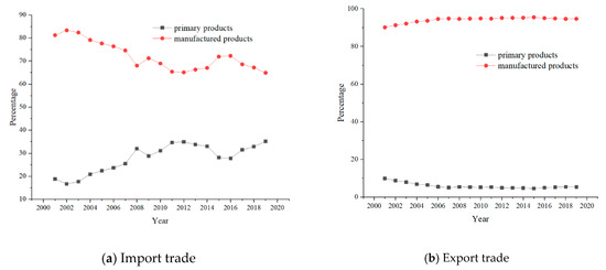
Figure 1.
The proportion of primary and manufactured products in (a) import and (b) export trade in China from 2001 to 2019. Source: official website of National Bureau of Statistics.
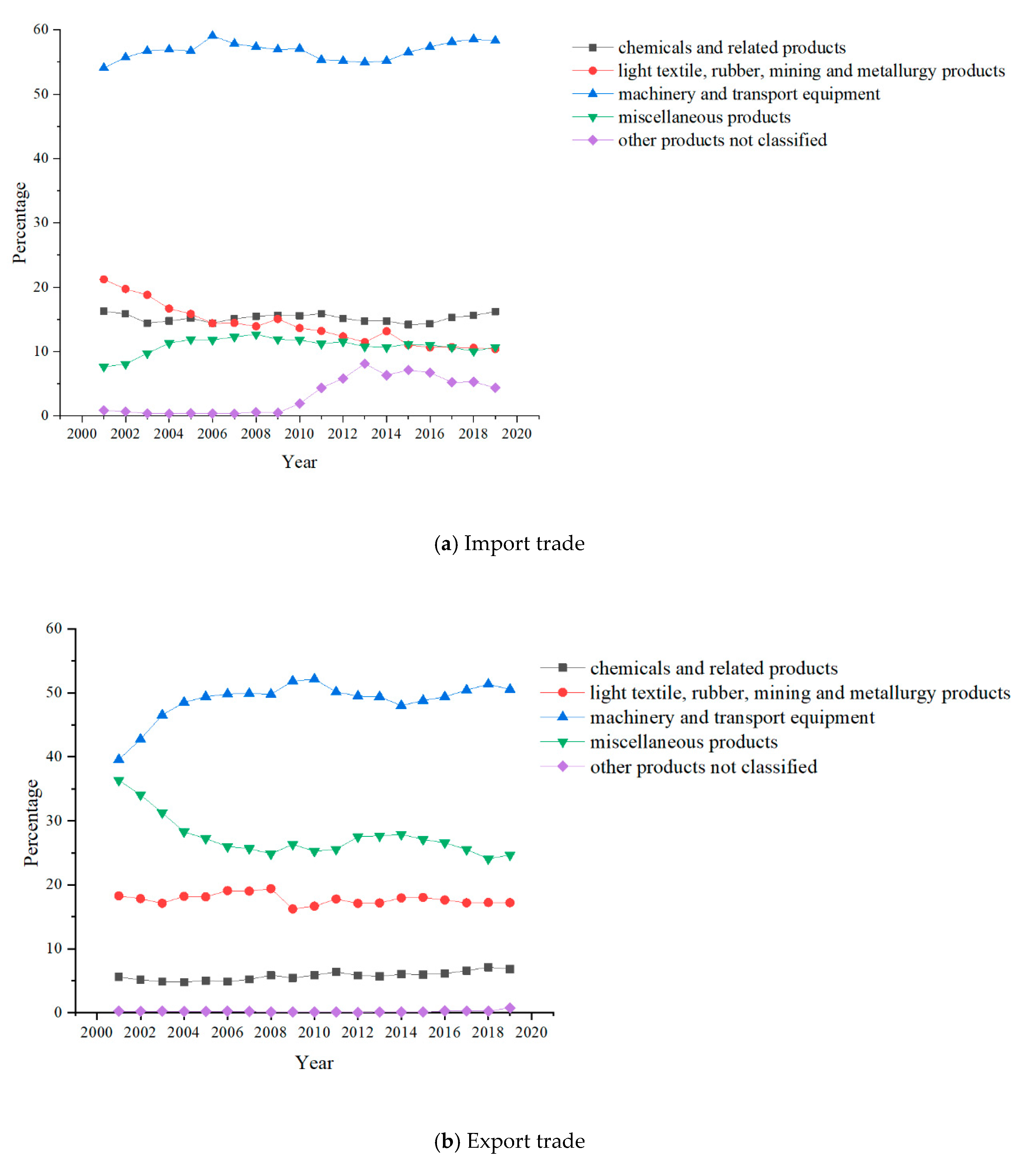
Figure 2 shows the variation curve of the proportion of the five types of manufactured products in the total manufactured products in international trade over time. For imports, the proportion of machinery and transport equipment slowly increased, and was a high proportion, as shown in Figure 2a. Notably, the proportion of light textiles and rubber products declined by about 10%. This could mean that the production of such products relies on domestic manufacturing, which would obviously contribute to CE. This may also be the reason why imports have a positive relationship with CE from the perspective of imported manufactured products. In exports, the share of machinery and transport equipment first increased significantly from 40% to about 50%, then fluctuated and increased slowly, while the corresponding share of miscellaneous products decreased from 35% to about 25%. The share of other types of manufactured products did not change significantly. Machinery and transportation equipment represent capital-intensive and technology-intensive products, while miscellaneous products are labor-intensive. Obviously, capital-intensive and technology-intensive products will bring much less pollution than labor-intensive products, and at the same time they bring more economic benefits. Therefore, the increase of this share is beneficial to the reduction of CE. In addition, more economic benefits also mean more funds for pollution control. In fact, exports may have a positive effect on CE when the regression corresponds to the year before 2000 due to the dominant position of miscellaneous products in our export structure.
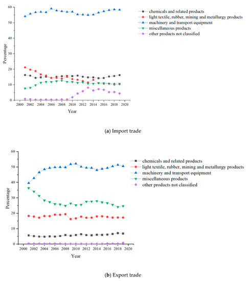
Figure 2.
The variation curve of the proportion of the five kinds of manufactured products in the total manufactured products with time in China for (a) import and (b) export trade. Source: official website of National Bureau of Statistics.
In the following, we will try to explain why the threshold effect exists and how it works. Although Figure 1 and Figure 2 represent the overall international trade situation of China in different years, they can also be regarded as the basic situation of cities with different levels of economic development to some extent. In other words, imports and exports in less developed cities are similar to those in earlier years, while imports and exports in developed cities are similar to those in recent years. Therefore, cities with more developed economies export more machinery and transportation equipment and less miscellaneous goods. The more developed cities will have more obvious negative effects on CE. From the imports point of view, developed cities will import more unclassified products, which may include science and technology products that are beneficial to pollution control. Moreover, they will also set higher industry standards for imported industrial materials. In general, the positive impact of import trade on CE may also turn negative after economic development.
5. Conclusions and Policy Implications
5.1. Conclusions
Based on the panel data of 282 cities in China from 2003 to 2016, the effects of import trade, as well as export trade, on CE were studied through linear regression and panel threshold regression analyses, and the following conclusions can be obtained:
- (1)
- Using the FE, FGLS and DK linear regression methods, it is found that import trade is positively correlated with CE, while export trade is negatively correlated with CE, and the influence of exports is obviously greater than that of imports.
- (2)
- The panel threshold regression analysis shows that there is a threshold effect on the relationship between imports, as well as exports, and CE. There exists one threshold with lnGDP as the threshold variable, while there are two thresholds when lnGIO is selected as a threshold variable. With the development of economy or industry, the effect of import trade will shift from increasing CE to curbing CE, while exports can continue to strengthen their role in reducing CE.
- (3)
- The mechanism of regression results is illustrated by the structure of China’s import and export trade. The positive impact of imports on CE is due to the increasing proportion of primary raw materials in China’s imports. The negative impact of exports on CE is due to the higher proportion of capital-intensive and technology-intensive products in exports, while labor-intensive products are in decline.
5.2. Policy Implications
On the basis of the above conclusions, the following policy recommendations can be made:
- (1)
- China should import less industrial raw materials and increase the proportion of imported high-tech products. After the introduction of advanced technology and equipment, the traditional high-emission industries will be upgraded based on digestion, absorption and transformation. Thus, the CE can be reduced while achieving economic growth.
- (2)
- China can further increase the proportion of capital-intensive and technology-intensive products in exports and reduce the proportion of labor-intensive products. Moreover, China should actively develop high-tech products, increase the added value of products, and make them strategic products for export. In addition, with global services trade growing significantly faster than trade in goods, China should expand the export of services.
- (3)
- Different trade policies should be determined according to different economic levels. For example, cities with less developed economies need to pay more attention to controlling CE in the import trade, and economically developed cities should continue to maintain and develop their control over CE in international trade.
Supplementary Materials
The following are available online at https://www.mdpi.com/article/10.3390/su13168968/s1, Table S1: List of Chinese cities.
Author Contributions
Conceptualization, J.W. and J.L.; methodology, J.W. and J.L.; software, J.W.; validation, J.W.; formal analysis, J.W.; writing—original draft preparation, J.W.; writing—review and editing, J.L.; visualization, J.W. and J.L. All authors have read and agreed to the published version of the manuscript.
Funding
This research received no external funding.
Institutional Review Board Statement
Not applicable.
Informed Consent Statement
Not applicable.
Data Availability Statement
The data used to support the findings of this study are available from the corresponding authors upon request.
Conflicts of Interest
The authors declare no conflict of interest.
References
- Friedlingstein, P.; O’Sullivan, M.; Jones, M.W.; Andrew, R.M.; Hauck, J.; Olsen, A.; Zaehle, S. Global Carbon Budget 2020. Earth Syst. Sci. Data 2020, 12, 3269–3340. [Google Scholar] [CrossRef]
- Dong, F.; Long, R.; Li, Z.; Dai, Y. Analysis of carbon emission intensity, urbanization and energy mix: Evidence from China. Nat. Hazards 2016, 82, 1375–1391. [Google Scholar] [CrossRef]
- Guan, D.; Peters, G.P.; Weber, C.L.; Hubacek, K. Journey to world top emitter: An analysis of the driving forces of China's recent CO2 emissions surge. Geophys. Res. Lett. 2009, 36, L04709. [Google Scholar] [CrossRef] [Green Version]
- Ren, S.; Yuan, B.; Ma, X.; Chen, X. The impact of international trade on China’s industrial carbon emissions since its entry into WTO. Energy Policy 2014, 69, 624–634. [Google Scholar] [CrossRef]
- Zhou, Y.; Fu, J.; Kong, Y.; Wu, R. How Foreign Direct Investment Influences Carbon Emissions, Based on the Empirical Analysis of Chinese Urban Data. Sustainability 2018, 10, 2163. [Google Scholar] [CrossRef] [Green Version]
- Wang, Y.; Liao, M.; Malik, A.; Xu, L. Carbon Emission Effects of the Coordinated Development of Two-Way Foreign Direct Investment in China. Sustainability 2019, 11, 2428. [Google Scholar] [CrossRef] [Green Version]
- Weber, C.L.; Peters, G.P.; Guan, D.; Hubacek, K. The contribution of Chinese exports to climate change. Energy Policy 2008, 36, 3572–3577. [Google Scholar] [CrossRef] [Green Version]
- Xu, X.; Mu, M.; Wang, Q. Recalculating CO2 emissions from the perspective of value-added trade: An input-output analysis of China's trade data. Energy Policy 2017, 107, 158–166. [Google Scholar] [CrossRef]
- Liddle, B. Consumption-Based Accounting and the Trade-Carbon Emissions Nexus in Asia: A Heterogeneous, Common Factor Panel Analysis. Sustainability 2018, 10, 3627. [Google Scholar] [CrossRef] [Green Version]
- Khan, Z.; Ali, M.; Jinyu, L.; Shahbaz, M.; Siqun, Y. Consumption-based carbon emissions and trade nexus: Evidence from nine oil exporting countries. Energy Econ. 2020, 89, 104806. [Google Scholar] [CrossRef]
- Zhang, C.G.; Lin, Y. Panel estimation for urbanization, energy consumption and CO2 emissions: A regional analysis in China. Energy Policy 2012, 49, 488–498. [Google Scholar] [CrossRef]
- Auffhammer, M.; Carson, R.T. Forecasting the path of China’s CO2 emissions using province-level information. J. Environ. Econ. Manag. 2008, 55, 229–247. [Google Scholar] [CrossRef] [Green Version]
- Yang, Y.; Cai, W.; Wang, C. Industrial CO2 intensity, indigenous innovation and R&D spillovers in China’s provinces. Appl. Energy 2014, 131, 117–127. [Google Scholar]
- Mi, Z.; Zheng, J.; Meng, J.; Zheng, H.; Li, X.; Coffman, D.M.; Woltjer, J.; Wang, S.; Guan, D. Carbon emissions of cities from a consumption-based perspective. Appl. Energy 2019, 235, 509–518. [Google Scholar] [CrossRef] [Green Version]
- Wang, Q.; Zhang, F. The effects of trade openness on decoupling carbon emissions from economic growth–Evidence from 182 countries. J. Clean. Prod. 2021, 279, 123838. [Google Scholar] [CrossRef]
- Eddine Chebbi, H.; Olarreaga, M.; Zitouna, H. Trade Openness and CO2 Emissions in Tunisia. Middle East Dev. J. 2011, 3, 29–53. [Google Scholar] [CrossRef]
- Fang, J.; Gozgor, G.; Lu, Z.; Wu, W. Effects of the export product quality on carbon dioxide emissions: Evidence from developing economies. Environ. Sci. Pollut. Res. 2019, 26, 12181–12193. [Google Scholar] [CrossRef]
- Mahmood, H.; Maalel, N.; Zarrad, O. Trade Openness and CO2 Emissions: Evidence from Tunisia. Sustainability 2019, 11, 3295. [Google Scholar] [CrossRef] [Green Version]
- Gozgor, G. Does trade matter for carbon emissions in OECD countries? Evidence from a new trade openness measure. Environ. Sci. Pollut. Res. 2017, 24, 27813–27821. [Google Scholar] [CrossRef]
- Ang, J.B. CO2 emissions, research and technology transfer in China. Ecol. Econ. 2009, 68, 2658–2665. [Google Scholar] [CrossRef] [Green Version]
- Qi, X.; Han, Y.; Kou, P. Population urbanization, trade openness and carbon emissions: An empirical analysis based on China. Air Qual. Atmos. Health 2020, 13, 519–528. [Google Scholar] [CrossRef]
- Li, B.; Liu, X.; Li, Z. Using the STIRPAT model to explore the factors driving regional CO2 emissions: A case of Tianjin, China. Nat. Hazards 2015, 76, 1667–1685. [Google Scholar] [CrossRef]
- Wang, Z.; Zhang, B.; Liu, T. Empirical analysis on the factors influencing national and regional carbon intensity in China. Renew. Sustain. Energy Rev. 2016, 55, 34–42. [Google Scholar] [CrossRef]
- Huang, J.; Hao, Y.; Lei, H. Indigenous versus foreign innovation and energy intensity in China. Renew. Sustain. Energy Rev. 2018, 81, 1721–1729. [Google Scholar] [CrossRef]
- Dou, Y.; Zhao, J.; Malik, M.N.; Dong, K. Assessing the impact of trade openness on CO2 emissions: Evidence from China-Japan-ROK FTA countries. J. Environ. Manag. 2021, 296, 113241. [Google Scholar] [CrossRef] [PubMed]
- Hasanov, F.J.; Khan, Z.; Hussain, M.; Tufail, M. Theoretical Framework for the Carbon Emissions Effects of Technological Progress and Renewable Energy Consumption. Sustain. Dev. 2021, 1–13. [Google Scholar] [CrossRef]
- Khan, Z.; Ali, S.; Umar, M.; Kirikkaleli, D.; Jiao, Z. Consumption-based carbon emissions and International trade in G7 countries: The role of Environmental innovation and Renewable energy. Sci. Total Environ. 2020, 730, 138945. [Google Scholar] [CrossRef]
- Liddle, B. Consumption-based accounting and the trade-carbon emissions nexus. Energy Econ. 2018, 69, 71–78. [Google Scholar] [CrossRef]
- Adebayo, T.S.; Rjoub, H. Assessment of the role of trade and renewable energy consumption on consumption-based carbon emissions: Evidence from the MINT economies. Environ. Sci. Pollut. Res. 2021, 1–13. [Google Scholar] [CrossRef]
- Shahbaz, M.; Gozgor, G.; Hammoudeh, S. Human capital and export diversification as new determinants of energy demand in the United States. Energy Econ. 2019, 78, 335–349. [Google Scholar] [CrossRef]
- Ahmed, K.; Ozturk, I.; Ghumro, I.A.; Mukesh, P. Effect of trade on ecological quality: A case of D-8 countries. Environ. Sci. Pollut. Res. 2019, 26, 35935–35944. [Google Scholar] [CrossRef]
- Yunfeng, Y.; Laike, Y. China's foreign trade and climate change: A case study of CO2 emissions. Energy Policy 2010, 38, 350–356. [Google Scholar] [CrossRef]
- Wang, S.; Li, C.; Ma, Y. Impact mechanism and spatial effects of urbanization on carbon emissions in Jiangsu, China. J. Renew. Sustain. Energy 2018, 10, 055902. [Google Scholar] [CrossRef]
- Kang, Y.-Q.; Zhao, T.; Wu, P. Impacts of energy-related CO2 emissions in China: A spatial panel data technique. Nat. Hazards 2016, 81, 405–421. [Google Scholar] [CrossRef]
- Liao, H.; Cao, H.-S. How does carbon dioxide emission change with the economic development? Statistical experiences from 132 countries. Glob. Environ. Chang. 2013, 23, 1073–1082. [Google Scholar] [CrossRef]
- Liang, W.; Gan, T.; Zhang, W. Dynamic evolution of characteristics and decomposition of factors influencing industrial carbon dioxide emissions in China: 1991–2015. Struct. Chang. Econ. Dyn. 2019, 49, 93–106. [Google Scholar] [CrossRef]
- Zhang, M.; Huang, X.-J. Effects of industrial restructuring on carbon reduction: An analysis of Jiangsu Province, China. Energy 2012, 44, 515–526. [Google Scholar] [CrossRef]
- Sun, Y.; Li, M.; Zhang, M.; Khan, H.S.; Li, J.; Li, Z.; Sun, H.; Zhu, Y.; Anaba, O.A. A study on China’s economic growth, green energy technology, and carbon emissions based on the Kuznets curve (EKC). Environ. Sci. Pollut. Res. 2021, 28, 7200–7211. [Google Scholar] [CrossRef] [PubMed]
- Nguyen, T.T.; Pham, T.A.T.; Tram, H.T.X. Role of information and communication technologies and innovation in driving carbon emissions and economic growth in selected G-20 countries. J. Environ. Manag. 2020, 261, 110162. [Google Scholar] [CrossRef]
- IPCC. 2006 IPCC Guidelines for National Greenhouse Gas Inventories; Institute for Global Environmental Strategies (IGES): Kanagawa, Japan, 2006. [Google Scholar]
- Huang, J.; Wu, J.; Tang, Y.; Hao, Y. The influences of openness on China's industrial CO2 intensity. Environ. Sci. Pollut. Res. 2020, 27, 15743–15757. [Google Scholar] [CrossRef]
- Hering, L.; Poncet, S. Environmental policy and exports: Evidence from Chinese cities. J. Environ. Econ. Manag. 2014, 68, 296–318. [Google Scholar] [CrossRef]
- Levin, A.; Lin, C.F.; Chu, C.S.J. Unit root tests in panel data: Asymptotic and finite-sample properties. J. Econom. 2002, 108, 1–24. [Google Scholar] [CrossRef]
- Im, K.S.; Pesaran, M.H.; Shin, Y. Testing for unit roots in heterogeneous panels. J. Econom. 2003, 115, 53–74. [Google Scholar] [CrossRef]
- Greene, W. Econometric Analysis, 4th ed.; Prentice Hall: Hoboken, NJ, USA, 2000. [Google Scholar]
- Wooldridge, J. Econometric Analysis of Cross Section and Panel Data; The MIT Press: Cambridge, MA, USA, 2002. [Google Scholar]
- Hoechle, D. Robust Standard Errors for Panel Regressions with Cross-Sectional Dependence. Stata J. Promot. Commun. Stat. Stata 2007, 7, 281–312. [Google Scholar] [CrossRef] [Green Version]
- Tang, X.; Jin, Y.; Wang, X.; Wang, J.; McLellan, B.C. Will China's trade restructuring reduce CO2 emissions embodied in international exports? J. Clean. Prod. 2017, 161, 1094–1103. [Google Scholar] [CrossRef]
- O'neill, B.C.; Dalton, M.; Fuchs, R.; Jiang, L.; Pachauri, S.; Zigova, K. Faculty Opinions recommendation of Global demographic trends and future carbon emissions. Proc. Natl. Acad. Sci. USA 2016, 107, 17521–17526. [Google Scholar] [CrossRef] [PubMed] [Green Version]
- Yang, T.; Wang, Q. The nonlinear effect of population aging on carbon emission-Empirical analysis of ten selected provinces in China. Sci. Total Environ. 2020, 740, 140057. [Google Scholar] [CrossRef] [PubMed]
- Hao, Y.; Ba, N.; Ren, S.; Wu, H. How does international technology spillover affect China's carbon emissions? A new perspective through intellectual property protection. Sustain. Prod. Consum. 2021, 25, 577–590. [Google Scholar] [CrossRef]
- Dong, F.; Wang, Y.; Su, B.; Hua, Y.; Zhang, Y. The process of peak CO2 emissions in developed economies: A perspective of industrialization and urbanization. Resour. Conserv. Recycl. 2019, 141, 61–75. [Google Scholar] [CrossRef]
- Hansen, B.E. Threshold effects in non-dynamic panels: Estimation, testing, and inference. J. Econom. 1999, 93, 345–368. [Google Scholar] [CrossRef] [Green Version]
- Hansen, B.E. Sample splitting and threshold estimation. Econometrica 2000, 68, 575–603. [Google Scholar] [CrossRef] [Green Version]

Publisher’s Note: MDPI stays neutral with regard to jurisdictional claims in published maps and institutional affiliations. |
© 2021 by the authors. Licensee MDPI, Basel, Switzerland. This article is an open access article distributed under the terms and conditions of the Creative Commons Attribution (CC BY) license (https://creativecommons.org/licenses/by/4.0/).