An Improved Forecasting Method and Application of China’s Energy Consumption under the Carbon Peak Target

Abstract

In the process of economic development, the consumption of energy leads to environmental pollution. Environmental pollution affects the sustainable development of the world, and therefore energy consumption needs to be controlled. To help China formulate sustainable development policies, this paper proposes an energy consumption forecasting model based on an improved whale algorithm optimizing a linear support vector regression machine. The model combines multiple optimization methods to overcome the shortcomings of traditional models. This effectively improves the forecasting performance. The results of the projection of China’s future energy consumption data show that current policies are unable to achieve the carbon peak target. This result requires China to develop relevant policies, especially measures related to energy consumption factors, as soon as possible to ensure that China can achieve its peak carbon targets.

1. Introduction

Energy consumption is tightly tied to the economic development of societies, and its importance is self-evident. China is currently the world’s largest energy consumer. In September 2020, China announced, for the first time, that it will achieve a carbon peak by 2030 and carbon neutrality by 2060 while optimizing its energy structure. The 14th five-year plan period is a critical period for China to reduce energy consumption and will lay a solid foundation for achieving a carbon peak by 2030 and carbon neutrality by 2060. China’s 14th five-year plan states that it will further reduce energy consumption in the industry to promote low-carbon development.

Therefore, how to accurately forecast energy consumption has become a key factor in policy making [1]. Renewable energy is always unpredictable [2,3], and its consumption also presents a fluctuating state. Therefore, this paper needs to solve the issue of how to establish a forecasting model with an accurate forecasting ability.

Thus far, scholars have proposed many forecasting models about energy consumption, and these models can be classified into three types: statistical models, gray models, and artificial intelligence models. Statistical models generally refer to regression models [4,5,6] and ARIMA models [7,8,9,10].

Aliyeh Kazemi et al., Carlos et al., and Ciulla et al. chose to use linear regression models to forecast various types of energy consumption [11,12,13]. However, statistical models have disadvantages such as easy underfitting, low forecasting accuracy, and the need for large sample data. Thus, gray models have been proposed.

Gray models [14,15] are widely preferred because the forecasting can be performed using only a small amount of data. Wang et al. proposed a seasonal gray model for forecasting solar energy consumption [16]. Yuan et al. and Zhou et al. forecast the energy consumption of China using a gray model [17,18]. However, this method is only suitable for approximating exponential growth forecasts, and the accuracy of medium- and long-term forecasts is poor.

Artificial intelligence algorithms can solve optimization problems well. At the same time, the results are accurate and rapid. Widely used artificial intelligence forecasting models include algorithmic models such as neural networks [19,20,21,22], support vector machines (SVMs) [23,24,25], and genetic algorithms [26,27,28]. Mailk et al. and Tian et al. used the neural network model to forecast building energy consumption [29,30]. Support vector machines improve generalization via the principle of structural risk minimization and can be extended to fields and disciplines such as forecasting and comprehensive evaluation [31]. A.S. reviewed artificial intelligence methods for building electrical energy forecasting models, such as SVM [32]. Xu et al. developed an SVM model for forecasting electrical energy consumption [33]. Support vector machine regression (SVR) is an important branch of application in SVM, which is widely used for time series forecasting. Iain et al. used SVR to forecast building energy consumption [34]. Bai et al. and Hu et al. used the SVR model to forecast natural energy consumption [35,36]. In order to enhance the accuracy of forecasting, numerous scholars have tried to use various optimization methods to optimize the parameters of SVR. Liu used VMD-GWO-SVR to forecast electricity daily load data [37]. Li used the IGSO algorithm to find the optimal parameters of SVR to obtain a forecast of air pollutant intensity [38]. Li proposed a joint IGWO-SVR algorithm for forecasting the battery health condition [39]. In a search of the literature, the authors found less studies on the use of the whale algorithm for SVR optimization, which is also a relatively new algorithm in recent years. Therefore, this paper chose to use the whale algorithm to optimize SVR, providing a new way of thinking for the optimization of SVR in the future.

Many scholars have improved and optimized the whale algorithm. Seyed et al. hybridized the WOA with the differential evolution algorithm, which has a better ability to explore function optimization, in order to overcome the disadvantage of premature convergence and local optimization [40]. Wang et al. optimized the whale algorithm by using the initialization strategy of Fuch chaotic mapping and oppositional learning [41]. Wu et al. proposed an improved whale optimization algorithm (ALWOA) based on adaptive weight and Levy flight to optimize the timing scheme of signalized intersections [42]. To improve the convergence speed and optimization capability of the algorithm, Xu et al. used a backward learning strategy, a nonlinear convergence factor, and adaptive weights to improve the whale algorithm [43]. Wang et al. improved the whale optimization algorithm (WOA) by replacing the linear parameter with a nonlinear rule [44]. Li et al. employed a nonlinear adjustment parameter and Gaussian perturbation operator in the whale optimization algorithm (WOA) [45]. It can be seen that many combinations of optimization methods have been adopted to improve the WOA, aiming at local and global searches.

Energy consumption forecasting is influenced by many factors [46,47,48,49]. The accuracy of the forecast value will influence the formulation of future policy; thus, this paper constructs an innovative and responsible forecast model. Based on the above methods, the linear SVR algorithm was used to forecast energy consumption, and the improved whale algorithm (IWOA) was used to optimize the model. The innovation points of this paper are as follows:

• In this paper, three methods, namely, compound chaotic mapping, nonlinear convergence factor, and local neighborhood disturbance, are used to optimize the whale algorithm in order to improve the search capability of the algorithm. By comparing the optimization ability of several optimization algorithms, the results show that the optimized whale algorithm has a strong optimization search ability.
• This paper presents an energy consumption forecasting model based on IWOA-linear SVR. The empirical analysis shows that the IWOA-linear SVR model has a higher accuracy, a stronger forecasting ability, and a better forecasting effect.
• This paper evaluates China’s 14th five-year plan and 2030 energy consumption target and puts forward relevant suggestions to provide a scientific basis for the formulation of an energy policy.

2. The Forecasting Model

2.1. Standard Whale Optimization Algorithm

The WOA (whale optimization algorithm) is a new swarm intelligence optimization algorithm proposed by Mirjalili and Lewis in 2016 [50]. In this paper, the algorithm was applied to optimize the parameters of a linear SVR, and its main steps are as follows:

1.

Prey surrounding

In the prey surrounding stage, the current local optimal solution is the individual closest to the food, and other individuals gradually approach the local optimal individual to surround the food. The mathematical model is as follows:

$$D=\left|C\cdot X^{*}\left(t\right)-X\left(t\right)\right|$$

(1)

$$X\left(t+1\right)=X^{*}\left(t\right)-A\cdot D$$

(2)

where $t$ is the number of current iterations, $X^{*}\left(t\right)$ is the current optimal individual position, $X\left(t\right)$ is the current individual position, $D$ denotes the gap between the optimal individual and the current individual, and $A$ and $C$ are coefficients. The formula is as follows:

$$A=2a\cdot r_1-a$$

(3)

$$C=2\cdot r_2$$

(4)

$$a=2\left(1-t/T_{\max }\right)$$

(5)

In Equations (3)–(5), $r_1$ and $r_2$ are uniformly distributed random numbers in the range [0, 1]; $a$ is the convergence factor, which linearly decreases; and $T_{\max }$ is the maximum number of iterations.

2.

Bubble net attacking

When a humpback whale attacks its prey, it renews itself in two ways: by contracting and by spiraling. When the coefficient vector is $\left|A\right|<1$, the algorithm searches for individuals to roam within the prey contraction envelope. At this point, the searching individual has a 50% probability of choosing to attack or to surround the prey. In the mathematical model, this can be expressed as follows:

$$X\left(t+1\right)=\left\{\begin{array}{ll}{X}^{\ast }\left(t\right)-A\cdot D& p<0.5\\ X^{\ast }\left(t\right)+D_P\cdot e^{bl}\cos \left(2\pi l\right)& p\ge 0.5\end{array}\right.$$

(6)

where $p$ is the probability of the algorithm choosing to attack or to surround the prey and is a random number in the range [0, 1], and $D_p$ is the distance between the individual and the prey. $b$ is a logarithmic spiral shape constant, and $l\in \left[-1,1\right]$.

3.

Searching for prey

Based on the variable coefficient $A$, when $\left|A\right|>1$, the whale swims outside the contraction envelope for a random search. The mathematical model is represented as follows:

$$X\left(t+1\right)=X_{rand}-A\cdot D^{\prime }$$

(7)

$$D^{\prime }=\left|C\cdot X_{\mathit{rand}}-X\left(t\right)\right|$$

(8)

where $X_{rand}$ represents a randomly selected position vector in the current population, and $D^{\prime }$ represents the distance between the search individual and $X_{rand}$, which is used by the search individual as a move step to update the position.

2.2. Improved Whale Optimization Algorithm

The WOA is a cluster intelligence algorithm. The basic WOA algorithm has the disadvantages of poor convergence and the tendency to fall into a local optimum. In the past, improvements to the whale algorithm mainly laid in the optimization of the regularization parameters. In this paper, the regularization parameter C and the tolerance coefficient Tol were selected for optimization. Meanwhile, most of the previous improvement methods were one or more combination methods of convergence factor and chaotic mapping. On this basis, two methods of composite chaotic mapping and nonlinear convergence factor were used in this paper. In particular, we added the local neighborhood perturbation method to enhance the local search capability of the algorithm.

1.

Compound chaotic mapping

Currently, the initial population of the whale algorithm is generated randomly, and the good degree of the initial population affects the efficiency of the algorithm; therefore, a comprehensive coverage of the search range can assist the algorithm in improving the convergence speed and accuracy.

Considering that chaotic operators are random and regular and can traverse all states without repetition in a certain range [51], this paper used tent mapping and logistic mapping for compounding to generate a search method for chaotic mapping, and this algorithm can improve the search efficiency in the prey encirclement phase. Compound chaotic mapping has a stronger local search capability [52].

The tent chaotic formula is as follows:

$$x_{n+1}=\alpha -1-\alpha \left|x_n\right|,-1<x_n\le 1,1<\alpha \le 2$$

(9)

The logistic chaotic formula is as follows:

$$x_{n+1}=\mu x_n\left(1-x_n\right),0<x_n<1,0<\mu \le 4$$

(10)

When $\alpha =2$, the Lyapunov exponent of the iterative equation of the tent mapping is the largest, and its chaotic orbit is most sensitive to the initial value. Based on this, the new mapping can be obtained by substituting the iteration series $x_{n+1}$ generated by bringing the tent mapping into the Lyapunov exponent in Equation (10) as the initial value $x_n$ of the tent mapping for compound iterations. The composite mapping is only a single full mapping when $1\le \mu \le 2$, and the sequence has boundedness and can enter the chaotic state. The formula is as follows:

$$x_{n+1}=1-2\mu x_n\left(1-x_n\right),0<x_n<1,1\le \mu \le 2$$

(11)

2.

Nonlinear convergence factor

In the original WOA algorithm, the linear convergence factor in the WOA algorithm tends to cause local stagnation. In order to efficiently search globally and locally, a combined convergence factor strategy is proposed, which is as follows:

$${\alpha }^{*}=\left\{\begin{array}{ll}\frac{1}{1{+e}^{2\cos \left(\frac{\pi }{2}\alpha \right)}}-0.11& \alpha <0.5\\ -{\log }_{10}\left(2\cos \left(\frac{\pi }{4}\alpha \right)\right)+0.3& \alpha \ge 0.5\end{array}\right.$$

(12)

where ${\alpha }^{\ast }$ from 2 to 0 shows a nonlinear decreasing trend, meaning that the convergence factor changes more in the early stage of the algorithm to strengthen the convergence speed and as far as possible to reduce the search range; later, the convergence factor changes less, increasing its local search efficiency to make the approximation of the lower bound more accurate.

3.

Local neighborhood disturbance

Throughout the iterative session of the whale algorithm, the optimal position is updated only when a better whale position appears, meaning that the possible optimal values in other regions are ignored. Since the optimal position may appear in a certain neighborhood of a position in the current population, a better optimization objective can be obtained by searching for the desired solution in the individual neighborhood, which, in turn, improves the convergence speed of the algorithm.

After generating each individual position, an individual is randomly selected to generate a surrounding disturbance to improve its judgment of searching in the nearby space, and this neighborhood disturbance is formulated as follows:

$$X^{\prime }=X+X\ast Poisson\left(\right)$$

(13)

where $Poisson\left(\right)$ is a random number satisfying the Poisson distribution, and $X^{\prime }$ is the new position generated.

For the generated neighborhood location, a greedy strategy is used to decide whether to use the location as the optimal location. The formula is given as follows:

$$X^{\ast }=\left\{\begin{array}{l}{X}^{\ast },f\left(X^{\ast }\right)\le f\left(X^{\prime }\right)\\ X^{\prime },f\left(X^{\prime }\right)<f\left(X^{\ast }\right)\end{array}\right.$$

(14)

In the formula, $f\left(X\right)$ is the position fitness of $X$, and $X^{\ast }$ is the original optimal position. Comparing the fitness of the original position with that of the new position, if the fitness of the new position is better, it becomes the current global optimal position. Otherwise, it stays the same.

2.3. Linear Support Vector Regression

In this paper, linear SVR was used as the forecasting model. The principle of linear support vector regression is as follows:

The training set is set to $\left(x_i,y_i\right)\left(i=1,2,3...,l\right)$, where $x_i\in R^n$ is the sample input, $y_t\in R^n$ is the sample output, and $l$ is the sample quantity. The loss function is set to an insensitive function.

The regression model is used to find a pair of parameters $\left(w,b\right)$ so that there is as little deviation as possible between the function $f\left(x_i\right)=w\cdot x_i+b$ and the actual target.

By introducing relaxation factors $\xi$ and ${\xi }^{\ast }$, we obtain the following:

$$\begin{array}{l}\min R\left(w,{\xi }_i,{\xi }_i^{\ast }\right)=\frac{1}{2}{‖w‖}^2+C{\displaystyle \sum _{i=1}^l\left({\xi }_i+{\xi }_i^{\ast }\right)}\\ \mathrm{subject}\mathrm{to}\left\{\begin{array}{l}{y}_i-w\cdot x_i-b\le \epsilon +{\xi }_i\\ w\cdot x_i+b-y_i\le \epsilon +{\xi }_i^{\ast }\\ {\xi }_i,{\xi }_i^{\ast }\ge 0\end{array}\right.\end{array}$$

(15)

where $C$ is the penalty factor, and $w$ and $b$ are the regression coefficient and the intercept, respectively.

The Lagrangian function is introduced for simplification, and $w$ is obtained by the following formula:

$$w={\displaystyle \sum _{i=1}^l\left(a_i-a_i^{\ast }\right)}\cdot x_i$$

(16)

where $a_i$ and $a_i^{\ast }$ are Lagrangian multipliers. This leads to the linear regression function

$$f\left(x\right)={\displaystyle \sum _{i=1}^l\left(a_i-a_i^{\ast }\right)}\left(x,x_i\right)+b$$

(17)

where $b=y_j-{\displaystyle \sum _{i=1}^l\left(a_i^{\ast }-a_i\right)\left(x_i,x_j\right)+\epsilon ,j\in \left\{m\left|0<a_m<C\right.\right\}}$.

Due to the complexity and precision of the regularized parameter adjustment model, if the value is too high, the generalization of the model is worse. Conversely, this leads to a lower complexity of the model, which may be underfitted, and renders the model less effective. $Tol$ is the size of the error value to stop training: the smaller the error tolerance, the higher the accuracy. The larger $Tol$ is, the fewer times the function is calculated and the faster it is, but the accuracy of the result becomes smaller. In order to enhance the model accuracy, the IWOA algorithm was used to optimize the regularization parameter $C$ and the error $Tol$ and to then optimize the linear SVR.

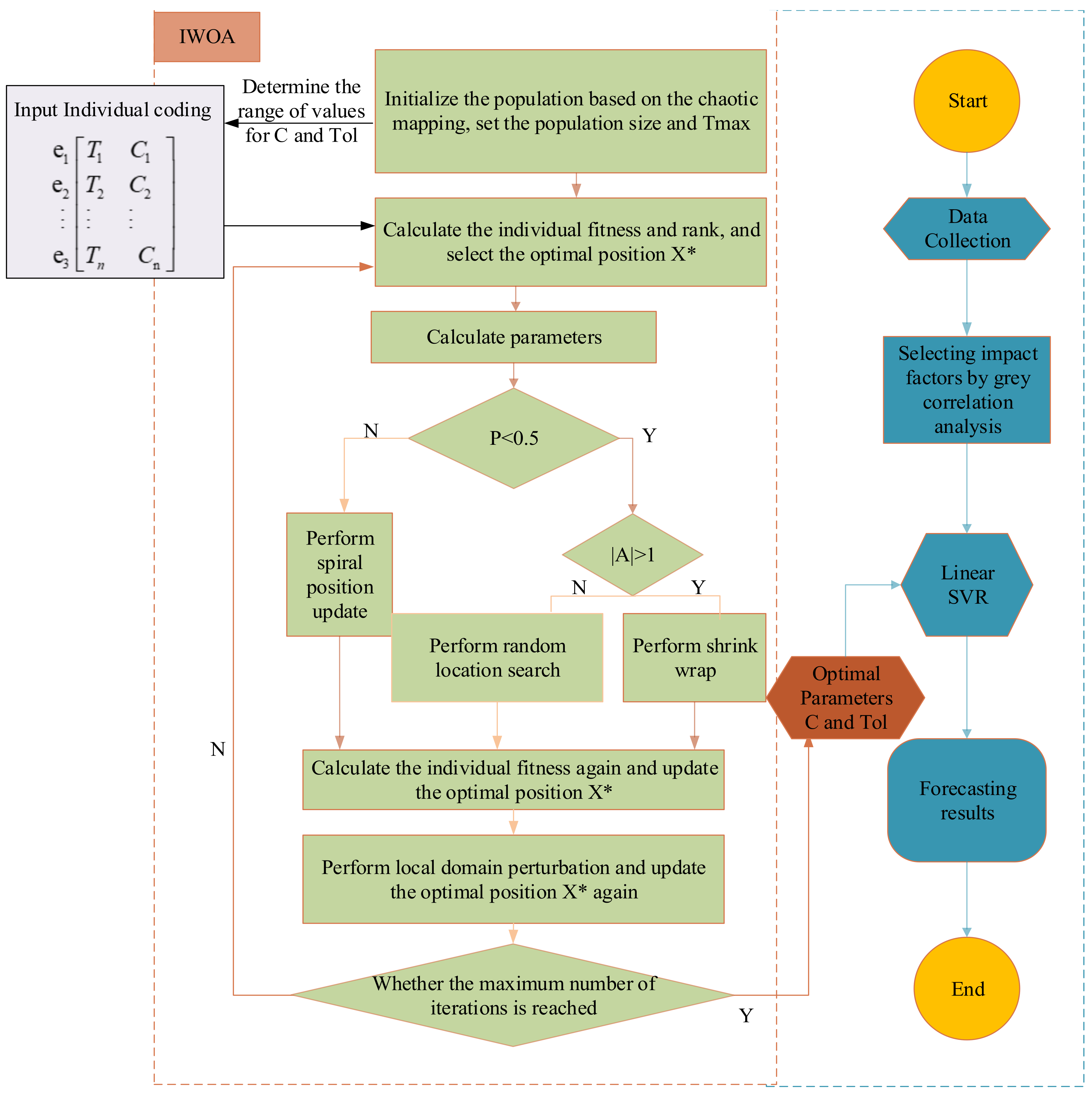
2.4. Improved Linear SVR Model Based on IWOA

In this paper, the IWOA was used to optimize the linear SVR in the following steps:

1.

Data processing

First, historical data were collected, and dimensionless data processing was carried out. Then, the gray relational analysis method was used to sort and screen the factors for the model input.

2.

IWOA-based linear SVR forecasting model

Based on 1, using the IWOA-linear SVR model, the forecast results for energy consumption were obtained. The specific steps are as follows:

Step 1: Set the population size $N$ and the maximum number of iterations $T_{\max }$ according to (11) to initialize the population algorithm. Determine the range of Tol and C.

Step 2: The population fitness is calculated according to the optimization problem, and the fitness values of each search individual solution are ranked to find the current optimal location $X^{\ast }$.

Step 3: The value of the nonlinear parameter $a$ is calculated and iterated according to Equation (12).

Step 4: Calculate the parameters $A$, $C$, $l$, and $P$. Determine whether the value of probability $P$ is less than 0.5. If yes, then go to Step 5; otherwise, search the individual and attack the prey in a spiral motion.

Step 5: Determine whether the value of the parameter $A$ is less than 1. If yes, the search individual reduces the amount they surround the prey; otherwise, the search agent conducts a global search.

Step 6: The fitness value of each individual is calculated again and compared with the location information $X^{\ast }$ of the optimal individual, and if it is better than $X^{\ast }$, the location of $X^{\ast }$ is replaced.

Step 7: An individual is randomly selected for the local search according to Equation (13), and the best individual retained is chosen according to Equation (14).

Step 8: Record the current number of iterations and compare it with the maximum number of iterations. If the set number of iterations is reached, terminate the iteration and output the current optimal solution; otherwise, return to Step 2 and continue the iteration.

Finally, the optimized parameters are assigned to linear SVR, and the forecasting model is built.

The forecasting process of the model is shown in Figure 1.

3. Experimental Analysis

3.1. Validation of Input Values for Forecasting Models

The data for this article are from the World Bank, National Bureau of Statistics of the People’s Republic of China, and BP’s World Energy Statistics Yearbook. This paper selects the factors that affect China’s energy consumption from 1990 to 2019, such as GDP, consumption level, import and export, coal proportion, population, industrial structure, urbanization rate, carbon emission, and energy intensity. In order to determine the model input value, this article uses the gray correlation method; the results are as follows:

The degree of correlation among the influencing factors is shown in

Table 1. Results of the gray relational analysis.

Influencing Factor	Gray Correlation Degree
GDP (billion yuan)	0.803017122
Consumption level of residents (yuan)	0.86801949
Total amount of imports and exports (billion yuan)	0.759810983
Energy consumption structure (%)	0.737780959
Population (m)	0.756403784
Industrial structure (secondary sector of the economy contribution to GDP (%))	0.718563884
Urbanization rate (%)	0.829549266
Carbon emissions (billion tons)	0.961802074
Energy consumption intensity (tce/ten thousand yuan)	0.651529903

. We chose a correlation degree above 0.7 as the input value of the forecasting model. The input factors are GDP, consumption level, import and export, energy consumption structure (coal proportion), population, industrial structure, urbanization rate, and carbon emission.

3.2. Performance Analysis of Optimization Algorithm

The IWOA-optimized performance comparing the 13 test functions, as shown in

Table 2. Single-mode reference function.

Function	Dim	Range	${\mathit{f}}_{\mathbf{min}}$
$f_1(x)={\displaystyle \sum _{i=1}^n{x}^2}$	30	[−100, 100]	0
$f_2(x)={\displaystyle \sum _{i=1}^n\left|x\right|}+{\displaystyle \prod _{i=1}^n\left|x_i\right|}$	30	[−10, 10]	0
$f_3={\displaystyle \sum _{i=1}^n{({\displaystyle \sum _{j=1}^n{X}_j^2})}^2}$	30	[−100, 100]	0
$f_4(x)={\max }_i\left\{\right|x_i|,1\le i\le n\}$	30	[−100, 100]	0
$f_5(x)={\displaystyle \sum _{i=1}^{n-1}[100{(x_{i+1}-x_i{}^2)}^2+{(x_i-1)}^2]}$	30	[−30, 30]	0
$f_6(x)={\displaystyle \sum _{i=1}^n({[x_i+0.5]}^2)}$	30	[−100, 100]	0
$f_7(x)={\displaystyle \sum _{i=1}^{n}i{x}_i{}^4+random[0,1]}$	30	[−128, 128]	0

;

Table 3. Multimode reference functions.

Function	Dim	Range	${\mathit{f}}_{\mathbf{min}}$
$f_8(x)={\displaystyle \sum _{i=1}^n-x_i\sin (\sqrt{\left|x_i\right|})}$	30	[−500, 500]	−418.98295
$f_9(x)={\displaystyle \sum _{i=1}^n[x_i{}^2-10\cos (2\pi x_i)+10]}$	30	[−5.12, 5.12]	0
$\begin{array}{l}{f}_{10}(x)=-20\exp (-0.2\sqrt{\frac{i}{n}{\displaystyle \sum _{i=1}^n{x}_i{}^2}})\\ -\exp (\frac{1}{n}{\displaystyle \sum _{i=1}^n\cos (2\pi x_i)})+20+e\end{array}$	30	[−32, 32]	0
$f_{11}(x)=\frac{1}{4000}{\displaystyle \sum _{i=1}^n{x}_i{}^2-{\displaystyle \prod _{i=1}^n\cos (\frac{x_i}{\sqrt{i}})+1}}$	30	[−600, 600]	0
$\begin{array}{l}{f}_{12}(x)=\frac{\pi }{n}\{10\sin (\pi y_1)+\\ {\displaystyle \sum _{i=1}^{n-1}{(y_i-1)}^2[1+10{\sin }^2(\pi y_{i+1})]}+{(y_n-1)}^2\}+\\ {\displaystyle \sum _{i=1}^{n}u(x_i,10,100,4)}\end{array}$ $y_i=1+\frac{x_i+1}{4}$ $u(x_i,a,k,m)=\left\{\begin{array}{c}\begin{array}{cc}k{(x_i-a)}^m& x_i>a\end{array}\\ \begin{array}{cc}0& -a<x_i<a\end{array}\\ \begin{array}{cc}k{(-x_i-a)}^m& x_i-a\end{array}\end{array}\right.$	30	[−50, 50]	0
$\begin{array}{l}{f}_{13}(x)=0.1\{{\sin }^2(3\pi x_1)\\ +{\displaystyle \sum _{i=1}^n{(x_i-1)}^2[1+{\sin }^2(3\pi x_i+1)]+{(x_n-1)}^2[1+{\sin }^2(2\pi x_n)]}\}\\ +{\displaystyle \sum _{i=1}^{n}u(x_i,5,100,4)}\end{array}$	30	[−50, 50]	0

was used to analyze the optimization performance of the IWOA, BA (bat algorithm), GWO (gray wolf algorithm), PSO (particle swarm optimization), and WOA (whale optimization algorithm). F₁–F₇ are unipolar functions that can be used to test the optimization speed of the algorithm. F₈–F₁₃ are multipolar functions that can be used to test the global search ability of the algorithm and to test the ability of the algorithm in escaping or avoiding falling into a local optimum.

The comparison is shown in

Table 4. Comparison results of algorithms.

Function	M × 10 tric	IWOA	BA	GWO	PSO	WOA
$f_1$	$avg$	2.48 × 10−208	2.49 × 101	7.44 × 100	2.29 × 102	6.66 × 108
	$stdv$	9.33 × 10−98	2.09 × 100	6.03 × 100	1.99 × 101	2.00 × 107
$f_2$	$avg$	3.00 ×10−136	3.21 × 101	1.36 × 104	4.95 × 101	2.04 × 10−95
	$stdv$	3.92 × 10−117	2.56 × 101	7.43 × 104	1.28 × 101	5.12 × 10−95
$f_3$	$avg$	7.05 × 10−205	6.29 × 101	1.95 × 103	4.03 × 102	1.08 × 10−188
	$stdv$	4.80 × 10−217	2.42 × 101	9.29 × 102	7.14 × 101	0.00 × 100
$f_4$	$avg$	2.62 × 10−185	3.90 × 100	1.41 × 101	4.54 × 100	1.78 × 10−19
	$stdv$	4.93 × 10−180	3.60 × 101	3.09 × 100	3.65 × 101	4.88 × 10−19
$f_5$	$avg$	2.21 × 10−63	6.11 × 103	2.34 × 103	1.89 × 105	3.96 × 101
	$stdv$	0.61 × 10−227	1.86 × 103	3.31 × 103	4.21 × 104	4.29 × 101
$f_6$	$avg$	5.43 × 10−166	2.73 × 101	6.54 × 100	1.54 × 102	2.83 × 100
	$stdv$	9.94 × 10−143	1.78 × 100	5.90 × 100	1.89 × 101	1.03 × 100
$f_7$	$avg$	9.85 × 10−175	2.33 × 101	1.32 × 102	1.57 × 102	3.11 × 105
	$stdv$	3.27 × 10−215	9.47 × 100	5.50 × 103	2.79 × 101	5.15 × 105
$f_8$	$avg$	0.76 × 10−146	−7.29 × 103	−7.51 × 103	−6.87 × 103	−5.22 × 103
	$stdv$	7.32 × 10−238	8.25 × 102	9.53 × 102	8.67 × 102	7.93 × 102
$f_9$	$avg$	2.75 × 10−211	2.31 × 102	9.71 × 101	3.65 × 102	0.00 × 100
	$stdv$	0.46 × 10−155	3.94 × 101	3.31 × 101	3.56 × 101	0.00 × 100
$f_{10}$	$avg$	8.92 × 10−241	6.29 × 100	4.71 × 100	8.21 × 100	4.24 × 10−16
	$stdv$	4.27 × 10−54	4.63 × 100	2.63 × 100	3.25 × 101	0.00 × 100
$f_{11}$	$avg$	4.33 × 10−95	5.36 × 10−1	7.24 × 101	1.03 × 100	0.00 × 100
	$stdv$	8.27 × 10−239	7.32 × 10−2	2.34 × 101	4.82 × 103	0.00 × 100
$f_{12}$	$avg$	6.72 × 10−164	2.38 × 101	8.82 × 100	4.94 × 100	1.81 × 101
	$stdv$	3.35 × 10−93	7.68 × 100	3.88 × 100	4.28 × 101	2.78 × 102
$f_{13}$	$avg$	5.23 × 10−249	2.23 × 100	3.25 × 101	3.58 × 101	4.78 × 100
	$stdv$	8.75 × 10−103	3.65 × 10−1	2.93 × 101	5.13 × 100	4.29 × 101

. Each test function records the global optimal solution obtained using each of the five algorithms and obtains the average value and standard deviation. The algorithm was programmed in Python 3.7.9. The basic parameters of the algorithm are as follows: the population size was set to 30, the maximum iteration of the algorithm was set to 500, each algorithm was run 30 times independently, and the average value and standard deviation of the results were obtained.

The experimental results show that the mean value reflects the convergence accuracy of the optimization algorithm, and the standard deviation reflects the stability. As it can be seen in the table above, the results of the IWOA for all 13 test functions are better than those of the other four algorithms, which indicates that the IWOA has a better optimization performance and robustness.

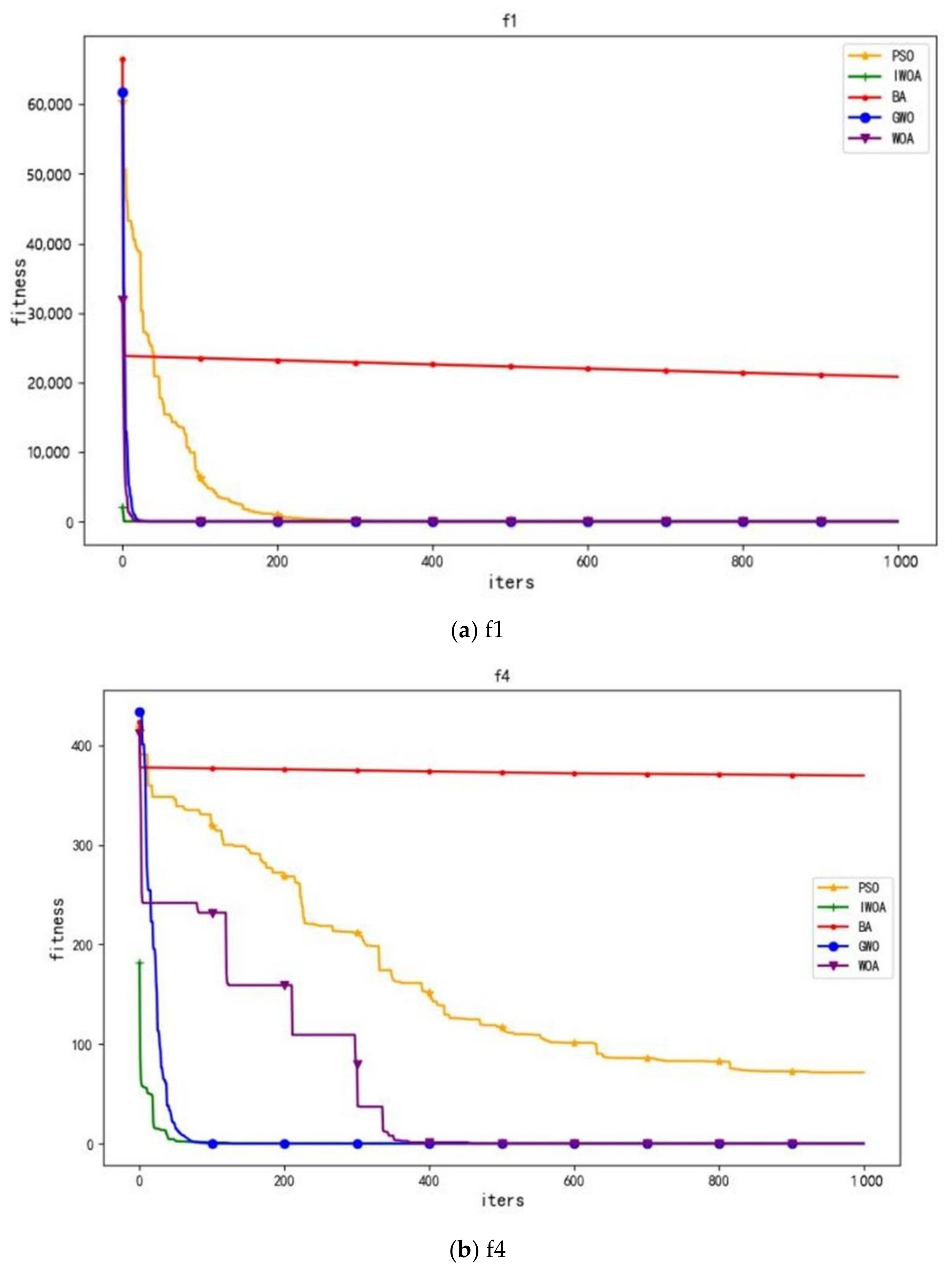
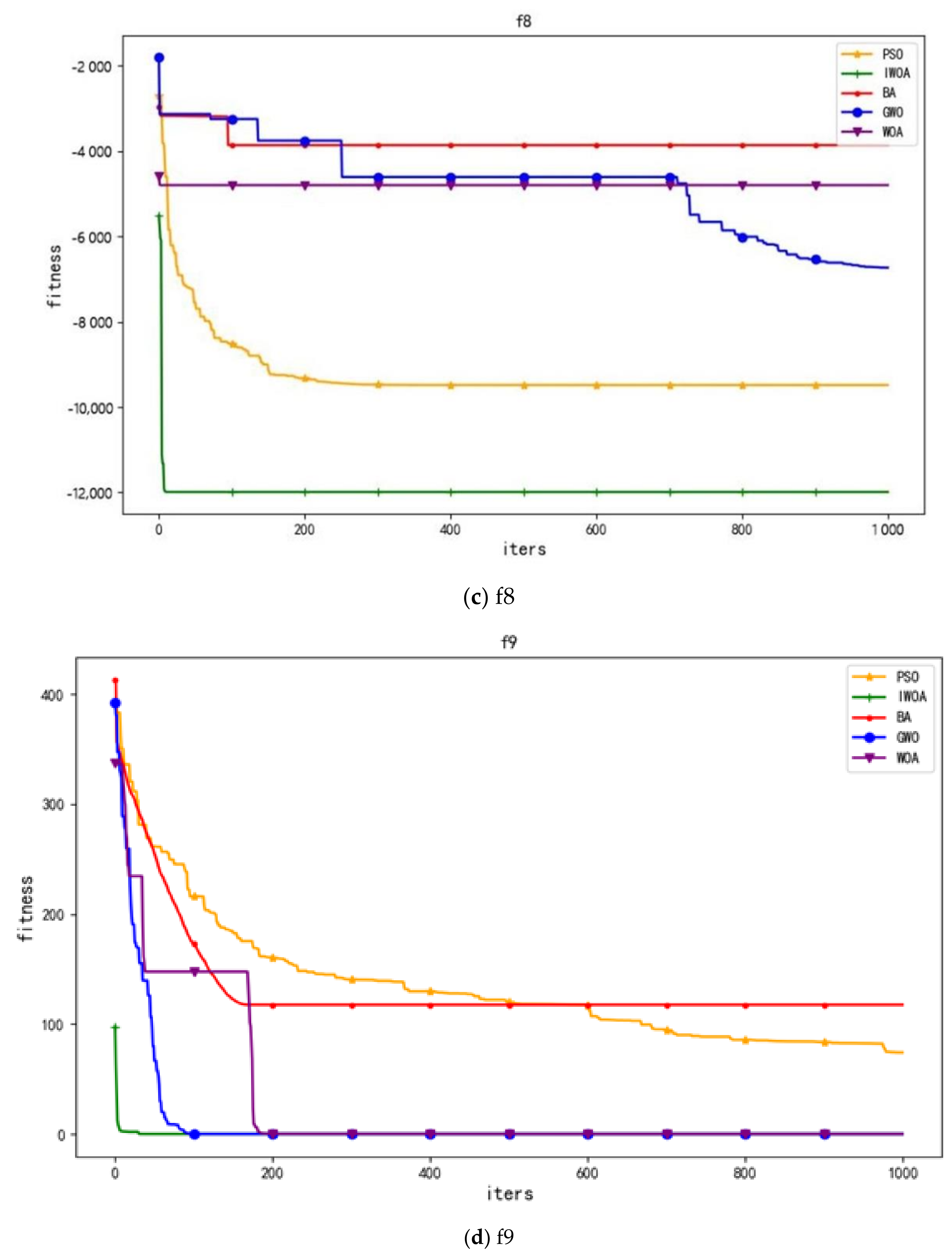
In this paper, four representative convergence graphs were selected, as shown in Figure 2. As it can be seen in the convergence curve of Figure 2, the IWOA has the fastest search speed for optimization, can effectively save search time, and has the best ability in obtaining the optimal solution.

In order to prove the effectiveness of the IWOA compared to linear SVR, the WOA, BA, GWO, and PSO were selected to optimize linear SVR, and the results of the parameter optimization were compared. The optimization results are shown in

Table 5. Results of the algorithm optimization (linear SVR stands for SVR).

	IWOA-SVR	WOA-SVR	BA-SVR	GWO-SVR	PSO-SVR
R2 Score	98.46%	97.86%	98.21%	97.41%	98.33%
Tol	0.007336	1.256905	0.000001	1.245675	0.000001
C	1.031752	0.000030	200.0000	0.000030	136.400593

.

The algorithm parameters were set as shown in

Table 6. Linear SVR algorithm parameter setting.

Metrics	Range
Tol	[10−6, 200]
C	[10−6, 200]
Maxiter	1000
dim	2

.

In this paper, R² was chosen as the criterion to judge the model. The formula is as follows:

$$R^2=1-\frac{{\displaystyle \sum _{i=1}^n{\left({\widehat{y}}_i-y_i\right)}^2}}{{\displaystyle \sum _{i=1}^n{\left({\overline{y}}_i-y_i\right)}^2}}$$

(18)

R² has a value range of [0, 1]. If the result is 0, the model fits poorly; if the result is 1, the model has no errors. R² is a non-unit, can be compared with other values of itself, and can be used to judge the goodness of fit intuitively; therefore, this paper chose it as an index to evaluate the fit degree of the model.

The closer R² is to 1, the better the model is, which means the closer we are to obtaining a perfect fit. According to the running results, IWOA-linear SVR is the best model, with the result closest to 1. According to the ranges of Tol and C, the TOL values of BA-SVR and PSO-SVR were too small, and their C values were too large, while the TOL values of WOA-SVR and GWO-SVR were within the normal range, but their C values were too small. Taken together, the IWOA had the best optimization capabilities for linear SVR.

3.3. Energy Consumption Forecast of China Based on IWOA-Linear SVR

In the process of model building, we need to divide the dataset into a training set, a verification set, and a test set to train the model. After the training, the final result of the test set is used to judge the model, but this may lead to the model over-fitting.

The k-fold cross-validation method can effectively reduce over-fitting of a model in a given dataset. The sample data before 2010 were divided into the training set and the verification set at a ratio of 4:1, and the remaining sample data were used as the test set, each time using the five groups of sample data as the training data and the remaining group of sample data as the verification set for a total of five times, in order to use the average accuracy to verify the model. As the sample data in this study are small, we adopted five-fold cross-validation for every model, in which each group has 4 samples, the training set has 16 samples, and the validation set has 4 samples.

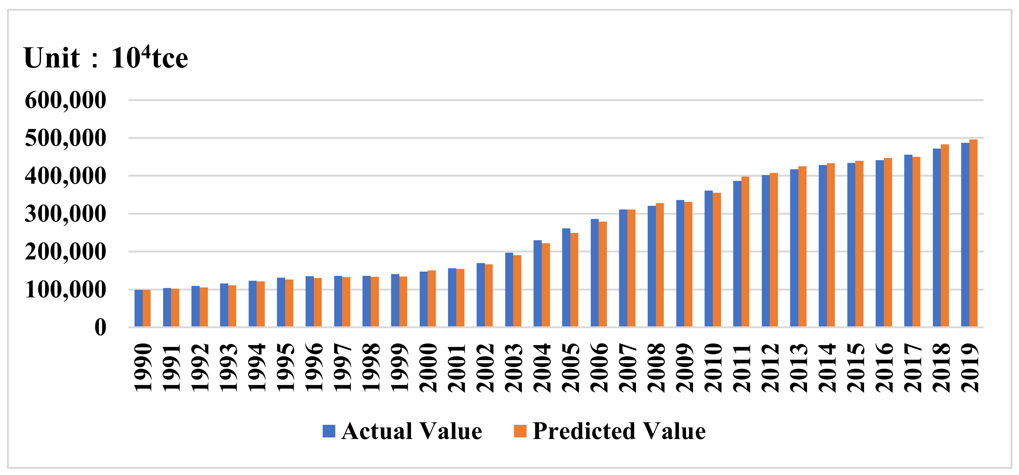
The forecasting result is shown in Figure 3.

The formula for calculating the relative error RE is expressed in Equation (18):

$$RE=\frac{\left|{\hat{y}}_i-y_i\right|}{y_i}\times 100\%$$

(19)

From

Table 7. Relative error.

Year	Actual Value (104 tce)	Forecasted Value (104 tce)	RE (%)
1990	98,703	98,634.54104	0.07%
1991	103,783	101,882.978	1.83%
1992	109,170	105,291.1203	3.55%
1993	115,993	110,986.8893	4.32%
1994	122,737	121,327.2492	1.15%
1995	131,176	126,172.5499	3.81%
1996	135,192	129,928.0744	3.89%
1997	135,909	132,376.0608	2.60%
1998	136,184	133,092.8162	2.27%
1999	140,569	133,879.844	4.76%
2000	146,964	150,053.6495	2.10%
2001	155,547	154,280.0707	0.81%
2002	169,577	166,275.3759	1.95%
2003	197,083	190,538.2778	3.32%
2004	230,281	222,118.2106	3.54%
2005	261,369	249,098.2486	4.69%
2006	286,467	279,338.404	2.49%
2007	311,442	311,442	0.00%
2008	320,611	327,829.134	2.25%
2009	336,126	331,495.7319	1.38%
2010	360,648	354,960.8872	1.58%
2011	387,043	397,999.9939	2.83%
2012	402,138	407,721.7381	1.39%
2013	416,913	425,209.2542	1.99%
2014	428,334	432,942.4791	1.08%
2015	434,113	439,790.7166	1.31%
2016	441,492	447,348.5768	1.33%
2017	455,827	450,341.9307	1.20%
2018	471,925	483,438.5672	2.44%
2019	487,000	496,422.0153	1.93%

and Figure 3 above, the forecasting curve of energy consumption using the IWOA-linear SVR model fits well with the actual curve. The relative error between the forecasted value and the real value is less than 5%, and the forecasting effect is remarkable.

3.4. Model Comparison and Error Analysis

In addition to the optimization ability of the algorithm, the optimal forecasting ability of IWOA-linear SVR needs to be proven. Five other models were selected, and the same sample data were used for the comparison with the IWOA-linear SVR model. The comparison results show that the IWOA-linear SVR forecasting results are, indeed, more accurate (the following graph abbreviates linear SVR as SVR).

Figure 4 shows the degree of fit between the forecasted and actual values of the different models. The IWOA-linear SVR model is most suitable for the actual curves.

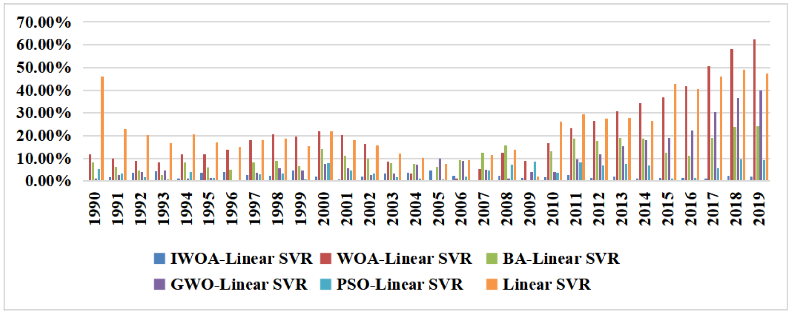
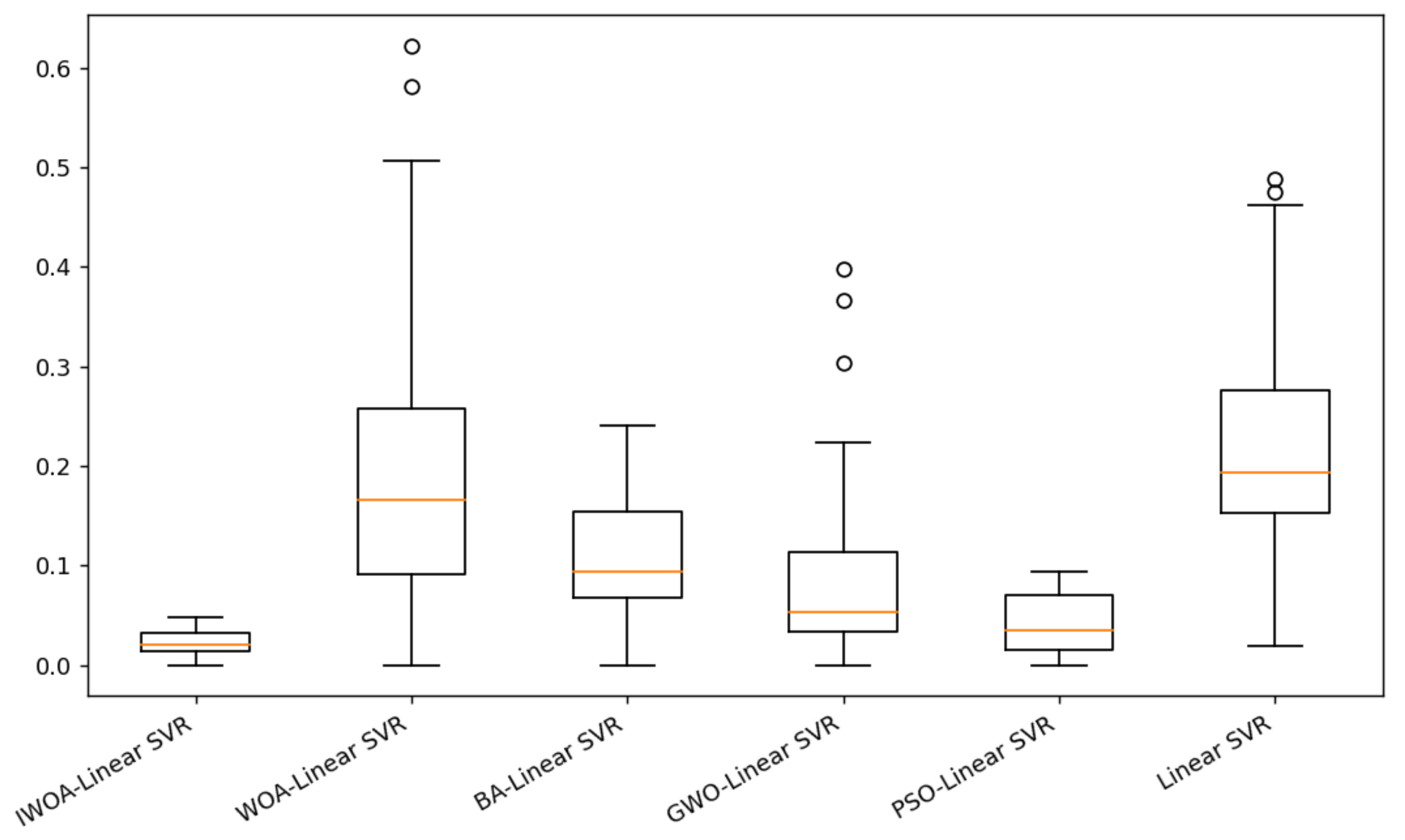
From Figure 5 and Figure 6, the IWOA-linear SVR model has a minimum relative error, followed by the PSO-linear SVR model; the other models have the maximum relative error.

In order to objectively evaluate the forecasting effect of each model, MAPE (mean absolute percentage error), RMSE (root mean square error), and MAE (mean absolute error) were used to compare the forecasting accuracy.

The mean absolute percentage error (MAPE) is one of the most popular metrics used to evaluate the performance of a forecast. The smaller the value, the smaller the error.

The root mean square error (RMSE) actually describes a degree of dispersion, not an absolute error. It measures the deviation of the observed value from the true value. The smaller the RMSE value, the better the model.

The mean absolute error (MAE) represents the mean of the absolute error between the predicted value and the observed value. The smaller the MAE value, the better the quality of the model, and the more accurate the prediction.

The formulae are as follows:

$$MAPE=\frac{1}{n}{\displaystyle \sum _{i=1}^n\left|\frac{{\hat{y}}_i-y_i}{y_i}\right|}$$

(20)

$$RMSE=\sqrt{\frac{1}{n}{{\displaystyle \sum _{i=1}^n\left({\widehat{y}}_i-y_i\right)}}^2}$$

(21)

$$MAE=\frac{1}{n}{\displaystyle \sum _{i=1}^n\left|{\hat{y}}_i-y_i\right|}$$

(22)

From

Table 8. Calculation results (the following table abbreviates linear SVR as SVR).

	IWOA-SVR	WOA-SVR	BA-SVR	GWO-SVR	PSO-SVR	Linear SVR
MAPE (%)	3.12251047	20.48030982	11.24815323	9.682133379	4.169042243	21.84254
RMSE (107 tce)	12.74570998	108.090835	49.01393016	63.06827405	18.69665672	541.2087053
MAR (104 tce)	91.91958034	262.1260115	189.0318169	190.7988472	113.8909016	590.2436011

, the MAPE, RMSE, and MAE of the IWOA-linear SVR models are the smallest among all models, reaching 3.12%, 12.75%, and 91.91, respectively. The next smallest is the PSO-linear SVR model: MAPE, RMSE, and MAE are 4.17%, 18.70, and 113.89, respectively. The maximum values of MAPE, RMSE, and MAE for the linear SVR model are 21.84%, 541.208, and 590.24, respectively. By comparison, we can see that the three indicators have the same trend. The three indexes of linear SVR all show minimum values, which proves that the model is superior to other models in the prediction precision. Therefore, it can be concluded that the IWOA-linear SVR model is superior to the other algorithms.

4. Energy Consumption Forecast of China in 2020–2030

The forecasting accuracy of the model was confirmed in the error analysis in the previous section. Next, the paper predicts the total energy consumption in China for 2020–2030 to realize the significance of the model. The targets and measures formulated during the period 2020–2025 lay a foundation for achieving the goals of a “carbon peak” and “carbon neutrality”. The energy intensity will be reduced by 13.5% during the fifteenth period according to the government’s work report. The National Development and Reform Commission set a target of 7.5 billion tons of coal for energy consumption by 2030. Based on this, this paper used IWOA-linear SVR to forecast China’s energy consumption data in 2025 and 2030 to judge whether China can achieve the target efficiently.

4.1. Impact Factor Analysis

In past research, some scholars only used the gray prediction method to predict the influencing factors and then obtain the future forecast value [53]. Before forecasting China’s energy consumption, it is necessary to combine China’s policy planning, to determine the changing trend of some influencing factors, and to then combine the gray forecasting method to obtain more accurate forecasting results.

1.

Energy consumption structure

At the UN Summit on Climate Ambition, Mr. Xi announced that China’s non-fossil fuels will account for twenty-five percent of primary energy consumption by 2030. This indicates that the energy structure will change greatly and that the proportion of coal will decrease rapidly.

2.

GDP

Affected by the COVID-19 pandemic, GDP growth in 2020 was 2.3%. At the annual GDP session for 2021, China set a target of 6% or more in GDP growth. Although the 14th five-year plan does not specify clear requirements for the speed of economic development, China currently faces downward pressure regarding the economy. As a result, GDP growth will be relatively flat.

3.

Consumption level of residents

The period 2021–2025 will be a critical period for China to move into a high-income country. Therefore, China will raise its national income level through policy liberalization. The income of the people is an important guarantee for the consumption level. Therefore, China’s consumption level will show a growth trend.

4.

Total imports and exports

The period of 2021–2025 will usher in a new phase in the development of “One Belt, One Road”. The double cycle of domestic and international creates new historical opportunities for the growth of trade. However, as the situation of the foreign “COVID-19” epidemic is still severe, China’s total import and export will enter a stable growth phase. With the easing of the “COVID-19” epidemic abroad, the growth of total import and export will be more rapid.

5.

Industrial structure

With the contribution rate of the service industry to economic growth increasing, there is great potential for the development of new business forms and new models. Over the next five years, the value-added share of China’s service sector will maintain a steady upward trend, expected to reach about 65%, and the manufacturing and service sectors will move towards a deep integration.

6.

Urbanization rate

China has proposed to improve its new urbanization strategy during the period 2021–2025. In his government work report, Premier Li Keqiang proposed that the urbanization rate of China’s resident population will increase to 65% by 2025. Based on this, China’s urbanization process will steadily advance.

7.

Population

The results of the seventh national census show that although the growth rate of China’s population will tend to slow down in the future, the total population will still be very large for a long time.

8.

Carbon emissions

China’s “carbon peak” target proposes to reach a carbon peak by 2030: by 2030, carbon emissions should reach their maximum. As a result, projections of carbon emissions will be affected.

As the other influencing factors have no definite policy objective, the other influencing factors are still forecast by the gray forecasting method.

Based on future trends in qualitative and quantitative analysis factors, we will be able to obtain a more accurate forecast of the total energy consumption from 2020 to 2035.

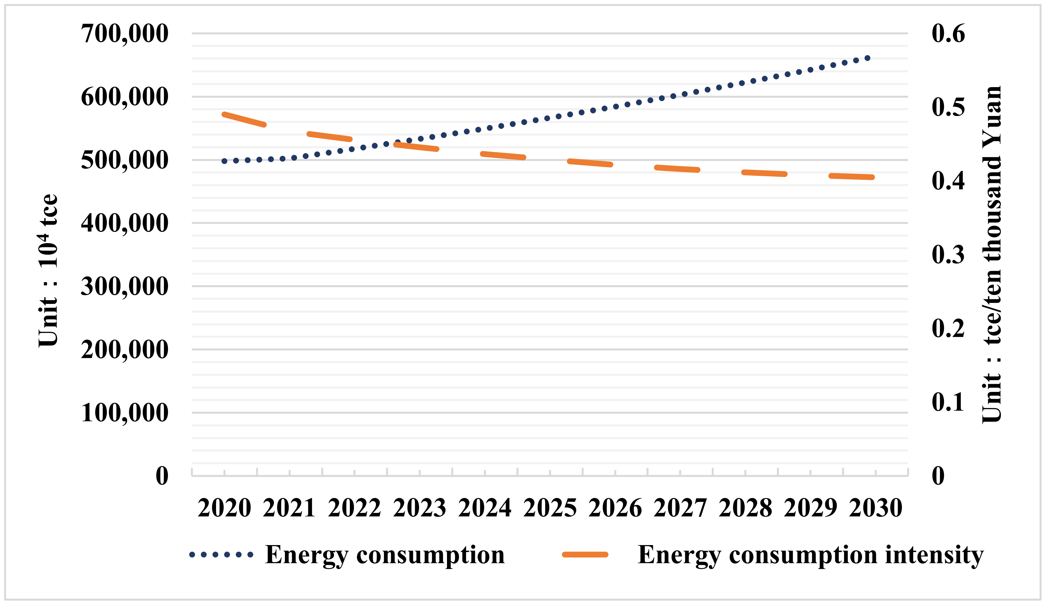
4.2. Forecast Results

According to the influencing factors set in Section 4.1, the IWOA-linear SVR model was used to forecast the energy consumption in China. The forecast results for 2020–2030 are shown in Figure 7 and

Table 9. Forecast results.

Year	Energy Consumption (104 tce)	Energy Consumption Intensity (tce/Ten Thousand Yuan)
2020	498,000	0.490164138
2021	502,141	0.46714554
2022	517,239	0.455673601
2023	532,961	0.445468936
2024	549,345	0.436467017
2025	566,422	0.428604837
2026	584,234	0.421834893
2027	602,818	0.416111961
2028	622,218	0.411401679
2029	642,479	0.407675589
2030	663,623	0.404896349

, and the forecast comparison results are shown in

Table 10. Forecast results.

Year	Total Energy Consumption (104 tce)	Energy Intensity (tce/Ten Thousand Yuan)	Whether We Can Achieve the Target of Energy Consumption Intensity of the 14th Five-Year Plan	Can We Meet the 2030 Total Energy Consumption Target
2020	489,000	0.490164138	——	——
2025	566,421	0.428604081	No	——
2030	663,623	0.404896349	——	Yes

Note: ——indicates that there are no targets set for that year.

.

The energy intensity formula is as follows:

$$Energyintensity=\frac{Totalenergyconsumption}{\mathrm{GDP}}$$

(23)

The forecasting results show that the total energy consumption will increase year by year, while the energy consumption intensity will decrease year by year.

Currently, China’s economy and society are experiencing high-quality development, and the future energy demand will continue to grow slowly. Therefore, the total energy consumption is rising in line with expectations.

The energy consumption intensity is an important index to measure the energy efficiency of a country. The lower the intensity of energy consumption, the higher the efficiency of energy utilization. China has been trying to reduce its energy intensity for years; therefore, the results are in line with the expectations.

According to Table 10, China can meet its 2030 energy consumption target, but it may fail to meet the energy intensity targets for the 14th five-year period.

Faced with a widespread shortage of energy supplies, the Chinese government has set a target of limiting total energy consumption to less than 7.5 billion tons of coal equivalent by 2030. In 2020–2030, the total energy consumption will show a steady growth trend. In 2030, total energy consumption will still be less than 7.5 billion tons of coal. As a result, China can meet its 2030 total energy consumption target.

The energy intensity will be reduced by 13.5% during the fifteenth period according to the government’s work report. This would mean that the energy intensity in 2025 would need to fall by 13.5% compared with 2020, while the figure based on Table 10 shows that it would only fall by about 12.6%. As a result, China is currently unable to meet its energy intensity target for the 14th five-year period.

Therefore, China needs to change its policies to achieve the energy intensity target.

5. Conclusions and Recommendations

We proposed a new IWOA-linear SVR model to accurately predict China’s energy consumption. The model has a high prediction accuracy and can describe China’s future energy consumption relatively accurately. The following conclusions can be drawn from this paper.

• Through gray correlation analysis, we can see that the value of energy consumption is closely related to carbon emissions and people’s affluence. In the future, we can start with low-carbon consumption when formulating energy saving and emission reduction policies.
• By comparing the IWOA with the WOA, GWO, BA, and PSO in optimizing linear SVR’s performance, the results of R² show that the IWOA has the best optimizing ability. By comparing the energy consumption prediction results and errors from 1990 to 2019, it shows that IWOA-linear SVR is more accurate than WOA-linear SVR, GWO-linear SVR, BA-linear SVR, PSO-linear SVR, and linear SVR.
• Due to the superiority of IWOA-linear SVR in the error comparison, the prediction results of energy consumption are of practical significance. Based on the forecast results for 2020–2030, China may not be able to achieve the energy intensity target of the 14th five-year plan under the established policies and national development plans, but it can meet its 2030 energy target.

Therefore, in order to achieve this target, China needs to take stronger measures to reduce energy consumption. This paper establishes relevant recommendations from the perspectives of both the individual consumer and the state.

From the perspective of individual residents, it is important to promote low-carbon consumption and to introduce the concept of low-carbon consumption. Low-carbon consumption includes low-carbon travel, low-carbon smart homes, and frugal consumption, contributing to the reduction in energy consumption in China through the efforts of individual consumers. The magnitude of energy consumption is positively correlated with people’s consumption. Actively guiding consumers to a low-carbon philosophy is conducive to the formation of a good atmosphere for energy conservation and low carbon and helps achieve the energy saving and emission reduction targets.

From the perspective of national policies and institutions, in addition to promoting the transformation of industrial structures and improving energy-saving technologies, subsidies from a low-carbon transition-related fund need to be set up by the state to favor high energy-consuming industries and resource-poor regions through special funding. At the same time, the state needs to implement carbon labeling for commodities, informing consumers about the carbon information of products in the form of labels.

Overall, this paper provides a practical energy consumption forecasting model, which provides a reliable tool for future energy consumption forecasting. As our model has strong prediction ability and needs less data, it can be widely used in the related research of energy prediction. In addition, this paper used the model to determine future targets, which can provide the scientific basis for national measures related to achieving the goal of reaching a “carbon peak”.