Abstract
Green spaces have a positive influence on human well-being. Therefore, an accurate evaluation of public green space provision is crucial for administrations to achieve decent urban environmental quality for all. Whereas inequalities in green space access have been studied in relation to income, the relation between neighbourhood affluence and remediation difficulty remains insufficiently investigated. A methodology is proposed for co-creating scenarios for green space development through green space proximity modelling. For Brussels, a detailed analysis of potential interventions allows for classification according to relative investment scales. This resulted in three scenarios of increasing ambition. Results of scenario modelling are combined with socio-economic data to analyse the relation between average income and green space proximity. The analysis confirms the generally accepted hypothesis that non-affluent neighbourhoods are on average underserved. The proposed scenarios reveal that the possibility of reaching a very high standard in green space proximity throughout the study area if authorities would be willing to allocate budgets for green space development that go beyond the regular construction costs of urban green spaces, and that the types of interventions require a higher financial investment per area of realised green space in non-affluent neighbourhoods.
1. Introduction
1.1. Access to Public Green Spaces and Quality of Life
With an expected population increase of 28% by 2060 [1], Brussels is facing the challenge of improving urban environmental quality [2] while absorbing strong demographic growth. A good understanding of access to Brussels’ public green spaces (GS) is required, as these are essential for the well-being and quality of life of the region’s inhabitants. This is not only important for the current state, but also for future development scenarios, as visiting urban green spaces has a general positive connection to reduced mortality [3], health protection [4], obesity in children and adults [5,6], and psychological well-being [7]. Next to mitigating impacts of air pollution and urban heat [8], reducing flood risk [9], and contributing to groundwater recharge [10], urban GS offer opportunities to reconnect with nature and self [11], resulting in a feeling of rejuvenation, enhanced contemplation, and a sense of peace and tranquillity [12,13,14,15]. Access to urban GS has a positive effect on the development and well-being of children [16] and may contribute to coping with a wide range of behavioural problems [17].
1.2. Green Space Accessibility Modeling
Standards and indicators for access to public GS come in many forms, and variations exist on the GS size levels that are taken into consideration and on the type of paths used for calculation (Table 1). GIS software is the prevailing tool for spatial analysis of GS accessibility. The simplest form—GS percentage or GS area per inhabitant—requires no distance calculation. The indicator has a low resolution and least reflects the inhabitant’s perception. When analysis is performed from the point of view of the inhabitant through focal (moving) neighbourhoods, access routes are either neglected and replaced by a unidirectional field (with barriers [18,19,20] or without barriers [21,22,23,24]), or a path/road network is considered [25,26,27,28]. One can also differentiate between road networks depending on the age of the users [29] (e.g., children and elderly having difficulty crossing specific roads). A public GS is considered accessible when the distance to it does not exceed the norm. To define this norm, some studies apply a single maximum distance [18,21,22,23,24,29], others stratify GS according to size classes [19,23,25,26,27,28], and a third—so far not implemented—approach is to have a maximum distance specific to, and as a function of, the GS area [20,25]. The most advanced models and indicators reflect user perception more by depicting paths and destinations more realistically [25,26,27,28]. Several studies use the GS accessibility models to analyse the relation between GS accessibility and socio-economic variables, such as well-being [18,22], age [21,29], education, and income [23]. Other studies use the models to analyse scenarios [24]. However, the influence of scenario developments on environmental justice (through socio-economic indicators) remains understudied.

Table 1.
Characteristics of green space accessibility models and indicators.
1.3. Unequal Distribution of Urban Green Space and Accessibility Benefits
In an urban context, GS provision is often unequally distributed [19,30]. Many studies reveal that GS accessibility predominantly benefits more affluent communities [31,32]. This is also the case for Brussels [25]. Disproportional access to green spaces is therefore increasingly recognized as an environmental justice issue [33]. Planners and policymakers are nowadays challenged, not only with the need to enhance the provision of GS across the city, but also with questions of justice regarding GS access and multi-functionality of GS, and provision of a healthy urban environment for all citizens. Recent studies have also highlighted the undesirable effects of urban greening, such as gentrification, whereby the added quality of urban green tends to ‘push out’ less affluent residents [34,35]. The benefits of bringing nature into neighbourhoods can be countered by destabilization of neighbourhoods through property value pressure, unequal access, and unequal benefits. For greening strategies to be inclusive, there has to be a deliberate acknowledgement of socio-spatial inequalities, and they have to be planned in a way that they can serve as places of encounter for different groups of people [34]. In this study, therefore, particular attention is paid to neighbourhoods with low average income.
The imperative to address environmental injustices and related health issues, as well as enhancing urban nature and biodiversity, has led planners to focus on traditional parkland acquisition programs, deployment of underutilized urban land, and defining innovative strategies for expanding green space resources [36]. Such open space development, however, can create an urban green space paradox in poor areas [33], where improved attractiveness increases property value. The average income in the BCR was €13,535 in 2013, which is 21% under the average Belgian income [37], with the lowest median incomes situated in the canal area. This is the historical industrial area, which is densely populated, and which has a low public green space proximity score. The highest median income areas are situated in the ‘second crown’ of the region and mostly in the southeast quarter of the area. The numbers do not include foreign diplomats, who have not been taken up in the national register.
1.4. Alternative Scenarios and Innovative Design Strategies
In all the challenges mentioned, the changing climate has agency. It not only forms but also alters the socio-political context in which GS and green infrastructure are developed [38]. To address these challenges, there is a strong interest in the formulation of design options, as well as in assessing the impact of alternative scenarios for urban GS development [39]. The preferred method for the formulation of design options/opportunities for GS development (OGSD) is collaborative design, supported by indicators of the current state of GS proximity. The co-production of scenarios through design and the impact assessment of alternative design options, along with the scientific and practical output it delivers, can be considered as research by design (RbD), that is, an inquiry in which design is a substantial part of the research process, forming a pathway to new insights through the inclusion of contextualized possible alternatives, validated through an interdisciplinary peer review of experts [40].
1.5. Objectives
The main objective of this paper is to present a GIS-based method for developing and analysing scenarios with a focus on environmental justice. This objective implies the identification of possible GS development scenarios for the Brussels’ study area and the assessment of how these scenarios benefit the population of Brussels as a whole, as well as different socio-economic segments of the population. The research reported in this paper makes use of the outcome of an earlier developed GIS model built for analysing the inherent quality of public GS [41] and proximity (accessibility) of public GS [25] from existing GIS data. The model is used in several ways: (a) the indicators are used for designing scenarios and strategies for public GS development for Brussels in RbD workshops and in additional RbD by the authors; (b) analysis of these scenarios (whether for single public GS or for the whole study area) is done through spatial and numerical comparison of the indicator scores; (c) this allows the formulation of design strategies and approaches for public GS development, as well as policy recommendations. The research presented is novel in its combination of three aspects: (a) high-resolution proximity indicators, calculated at the urban block level, using path network distances; (b) in-depth collaborative RbD exercises on opportunities for GS development; and (c) scenario-based impact analysis in relation to socio-economic indicators.
2. Materials and Methods
2.1. Concepts
The methodology involves concepts that are explained more in-depth first. The proximity model is the GIS-based model that was developed by the authors [25] for producing indicators for proximity of green spaces on different Theoretical Functional Levels (TFL). The notion of TFL relates the distance to GS that a resident is willing to cover to the size of the GS. The rationale behind this approach is that the size of a GS determines the range of functions or activities the GS may potentially support. It is assumed that residents will be prepared to cover longer distances to reach a larger GS, because of its improved offer in terms of amenities, potential uses, and benefits [25]. This idea is supported by several empirical studies [19,42]. In the proximity model used in this study, seven theoretical functional levels (TFL) are defined, from the residential to the metropolitan scale, each corresponding with a minimum size and maximum distance, the latter obtained empirically (Table 2, Figure 1). Design is used in this study to test possibilities for creating GS and for testing these propositions against the multiple preconditions concerning development of GS. GS that are proposed on suited locations as a solution for the lack of GS on a specific TFL are named Opportunities for Green Space Development (OGSD). When a specific set of OGSD is chosen for impact analysis, it is called a scenario.
Table 2.
Theoretical functional levels (TFL) with values used for the proximity modelling.
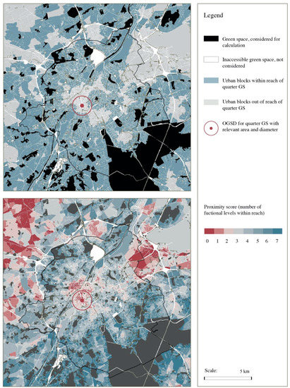
Figure 1.
Urban blocks within reach of quarter green space (top) and proximity score of urban blocks (bottom).
2.2. Materials
GS proximity is modelled according to the procedure described in Stessens, Khan, Huysmans and Canters [25] and its standards. A visual representation of the existing public GS and TFL Spatial indicators/maps produced by the model are calculated at the level of urban blocks and include identification of all urban blocks having a specific level of GS within reach (Table 2, Figure 2, top), as well as an overall proximity score ranging from 0–7, indicating for each urban block how many of the seven TFL are accessible (Figure 2, bottom). It is important to note that functional levels form a hierarchy, where it is assumed that higher-level GS also offer the functions of lower-level GS. For example, district GS are also considered in the calculation of access to neighbourhood green, applying the maximum distance threshold for the latter. For the design exercises, the proximity indicator maps (model output) were complemented with an aerial image of Brussels at 25 cm resolution. Additional layers that were used for location finding of new GS are: a base map including buildings, parcel boundaries, and existing GS (Figure 1), the public transport network (rail, metro, tram), surface water (streams and water bodies), protected landscapes and nature reserves, a noise map (road, rail, and air traffic), and the biological valuation map (Table 3).
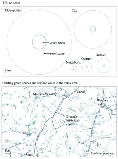
Figure 2.
Minimum TFL areas plotted as circles and outlines in the study area on the same scale. ↑ North.
Table 3.
Maps used for the design exercises and scenario development (all are in vector format, except for (*), which are in raster format).
2.3. Main Methodology
Table 4 provides an overview of the different steps in the methodology and the materials used in each step. The RbD was performed in two parts: (i) during an interdisciplinary workshop (Figure 3) with twelve participants, including researchers (e.g., architects and urban designers, planners, hydrologists, geographers), students in architecture and urban design, people from the regional office for environment, and regular citizens—here, proximity maps per TFL were projected on whiteboard for drawing GS development scenarios; (ii) during a smaller session (one researcher and one student) on GIS analysis, for processing the workshop outputs, and for additional scenario work. Complex solutions were further tested in AutoCAD. Based on the interventions needed for the realisation of the green space, OGSD were classified according to investment scale, from regular investment to high additional costs. The development options include both traditional GS planning options and more intricate options that can be considered in case a traditional solution is not spatially possible. One of the goals of the exercise is to explore which degree of complexity of solutions is needed to provide sufficient green space accessibility in the most challenging areas. The spatial as well as demographic impact was then assessed for the whole study area as well as for two socio-economic groups in the BCR.
Table 4.
Methodological steps and materials used.
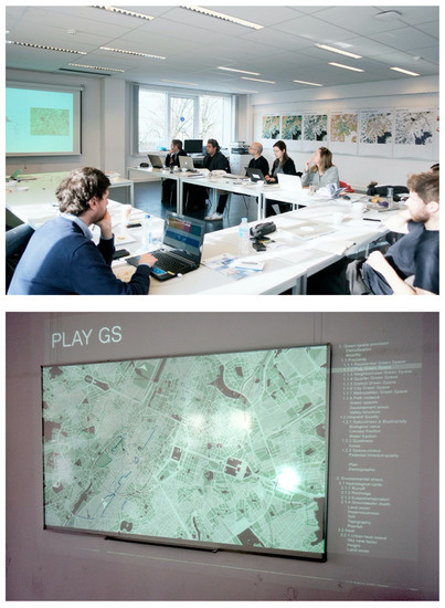
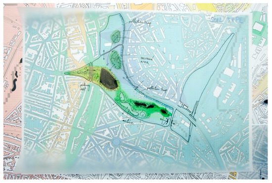
Figure 3.
Pictures of the collaborative RbD workshop. Top: plenary session and discussion; middle: joint sketching session of OGSD on projected media (output of proximity modelling); bottom: detailed design of one case study for expansion and improvement of an existing park.
2.4. Collaborative RbD Workshop
In the workshop, the study area was explored for public GS optimisation possibilities with the help of the output of the proximity model (Figure 2). Maps depicting the accessibility of each separate TFL were used for identifying opportunities/options for green space development (OGSD). OGSD comprise all viable options to develop public GS or to expand an existing public GS. They are outlined by a perimeter and involve spatial interventions. All interventions necessary for the OGSD to be feasible were then determined and listed. To determine the relevant interventions, rudimentary design exercises were made, such as drawing the perimeter on aerial imagery, overlay with other maps, or more detailed design exercises in case of complex potential public GS.
2.5. Individual RbD
Four questions are explored: (i) whether the study area can be fully served at all TFL; whether ‘standard’ approaches exist for GS development and how these differ for each TFL; which scenarios can be formulated based on the design exploration; and how do these scenarios relate to the earlier described correlation with socio-economic indicators?
3. Results
First, inequalities in the provision of GS in the BCR are briefly discussed, focusing on the proximity of GS of different functional levels. Next, the results of the RbD exercises for the improvement of GS proximity are discussed per TFL, and distinctive types and opportunities of GS creation are identified. In the last part, these OGSD are incorporated in three different scenarios, depending on how (financially) challenging different types of interventions are. In the scenario analysis, GS proximity for the poorest 25% of neighbourhoods is compared with scenario outcomes for other neighbourhoods.
3.1. Inequalities in Green Space Provision
As Figure 4 shows, green proximity scores, expressing the diversity of TFL within reach of each urban block, are generally higher in the periphery of the BCR than in the central parts of the city. Weighting the lack of GS (reversed proximity score multiplied with the population density) highlights the lack of GS in the densely populated 19th century belt around the centre of the BCR (Figure 5). Figure 6 and Figure 7 show the urban blocks within reach of a certain TFL of GS, and therefore also the gaps where GS of the specific TFL should ideally be provided. Whereas the gaps in residential and play GS proximity are quite fragmented, in the higher TFL, clear zones start to appear, with a consistent lack in the historical centre up to district GS and a north-south partitioning for city and metropolitan GS.
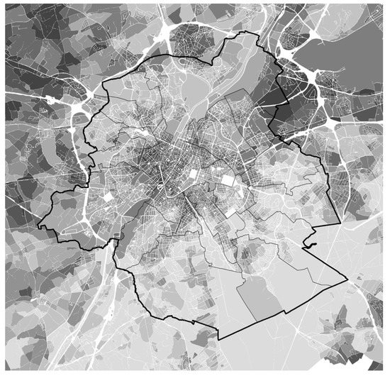
Figure 4.
Proximity score at urban block level (dark 0–7 light). Lines: Brussels-Capital Region (thick) and the 19 municipalities it is composed of (thin) ↑ North—Scale:  5 km.
5 km.
5 km.
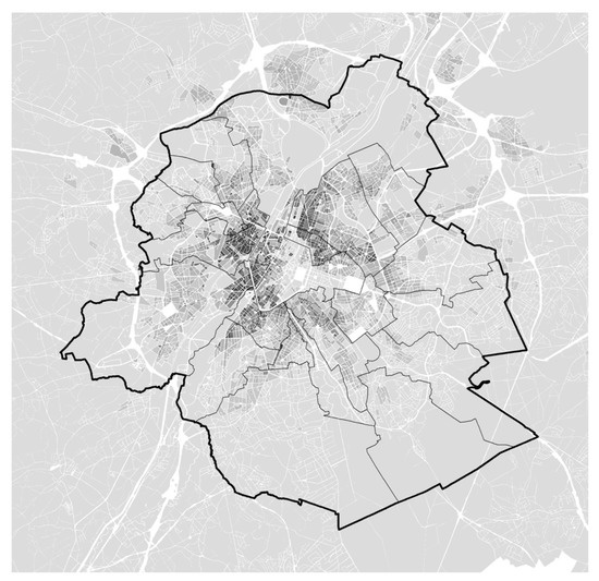
Figure 5.
Impact of lack of green space proximity (population weighted). Light: low impact; dark: high impact (i.e., low proximity
scores in densely populated areas). Lines: Brussels-Capital Region (thick) and the 19 municipalities it is composed of (thin) ↑ North—Scale: 5 km.
5 km.
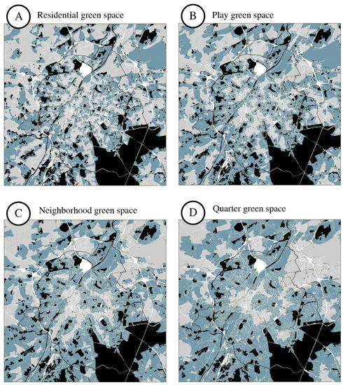
Figure 6.
Urban blocks within reach of seven levels of public green space (continues on the next page, including legend). Residential green space (A), play green space (B), neighborhood green space (C) and quarter green space (D).
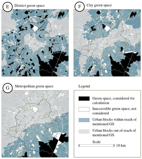
Figure 7.
Urban blocks within reach of seven levels of public green space (continuation of the previous page). ↑ North. District green space (E), city green space (F) and metropolitan green space (G).
3.2. Research by Design on Improvement of Public GS Proximity
In the design workshops, by means of the GS proximity indicators per functional level (Figure 6 and Figure 7), 162 OGSD were identified for the whole study area (Table 5, Table 6 and Table 7, Figure 8, Table A1, Table A2, Table A3, Table A4 and Table A5 in Appendix A) relating to the TFLs neighbourhood GS (level 3) to metropolitan GS (level 7). These OGSD were defined with the goal of increasing the amount of people within reach of a TFL with a minimum of interventions. By solving higher TFL first, starting with metropolitan GS, some OGSD could be considered redundant in lower levels, as they were already covered by the proposed GS on a higher level. For example, when introducing a metropolitan structure in the west of Brussels with a reach of 5900 m, an outward buffer zone of 707 m (theoretical displacement of 1000 m distance reach of district GS, see: displacement, Table 7) was taken into account. Here, in this area, the introduced metropolitan GS already covered the district GS proximity. The proposed OGSD are visualised relative to existing green spaces in Figure 8. For the study area as whole, the levels residential GS (level 1) and play GS (level 2) would potentially result in a very high amount of OGSD, and determining these is out of the scope of this work. Therefore, for these levels, a focus area was selected (Figure 8, dashed line), in which 42 OGSD were defined. In total, 53 types of interventions needed for the realisation of the proposed OGSD were identified (Table 5 and Table 6). For quarter green (level 4) up till metropolitan green (level 7), OGSD can be grouped into types according to recurring interventions (Table 5). For residential (level 1) up to neighbourhood green (level 3), interventions proposed are limited, so OGSD types are self-explanatory, referring to a particular type of intervention. Interventions proposed for all OGSD are listed in Appendix A (Table A1, Table A2, Table A3, Table A4 and Table A5). The following sections provide a description of common and specific interventions related to the different types of OGSD.
Table 5.
Number of and parameters related to proposed green spaces.
Table 6.
Types of GS development options (TFL residential-neighbourhood excluded as these are self-explanatory, as they are related to one intervention).
Table 7.
Interventions not related to specific GS typologies.
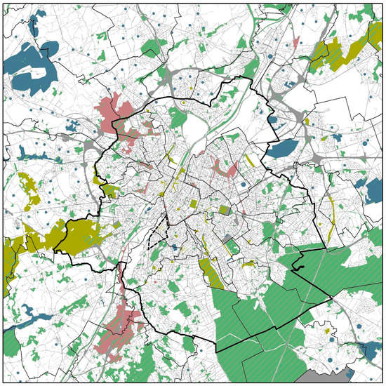
Figure 8.
Existing public GS (green) and
proposed public GS (blue: low investment; yellow: medium investment; red: high investment). Hatched GS are reconversions or expansions of existing GS. Dots are indications of green spaces without their actual shape. The size of the dot
represents its actual TFL area, which has been verified visually to fit in the landscape. Thick line: Regional border Brussels–Flanders, thin line: city borders, dashed line: focal area for residential and play GS OGSD. ↑ North—Scale: 5 km.
5 km.
3.3. Three Scenarios of PUBLIC GS Development
Three scenarios were created by selecting a subset of OGSD that were identified earlier in the process: basic investment (BASE); supplementary investment (SUPP); and full investment (FULL) (Table 8, detailed listing in Appendix A, spatial representation in Figure 8). Most OGSD require an additional investment apart from regular construction costs for public GS. The investment class of an OGSD determines in which scenario it is included. The classification is approximate due to the absence of detailed cost estimates, though sufficiently discriminating for its purposes, which is to define three public GS development scenarios based on approximate investment. The following cost-increasing actions were considered for the scenario classification: tunnel construction or similar works; above-ground infrastructure works; compulsory residential real estate acquisition; compulsory industrial/logistic real estate acquisition; altering public facilities; agricultural land acquisition; and installing noise barriers.
Table 8.
Number of OGSD per scenario per functional level of the proposed GS.
In the design exercises, the low-cost OGSD (suited for the BASE scenario) were given priority when deciding on locations for public GS development in the scenarios. An optimal allocation was pursued to introduce a minimum of OGSD for a maximum improvement of GS accessibility for each functional level. With these preconditions, for the FULL scenario where a maximum coverage is attempted, at least 43% of the proposed public GS are not low cost.
The current state of GS proximity is described in detail in Stessens, Khan, Huysmans and Canters [25]. To summarise, there is a strong lack of public GS in the area including East Molenbeek and the west of central Brussels (area marked as A in Figure 9) and to a lesser extent in Sint-Joost-Ten-Node (Figure 9B) and the Hallepoort-Louise-Matongé area (Figure 9C). A few patterns are the cause of this: (i) district GS is not present in the central parts of the BCR; (ii) city GS only occurs along the northwest and southeast border of the BCR, resulting in a southwest-northeast oriented axis with reduced accessibility to higher-level green spaces; and (iii) metropolitan GS is absent in the north, leaving the northern part of the BCR underserved [25]. Residential GS and play GS have more irregular patterns of coverage, yet are less well represented in dense urban areas, which in combination with the lack of other TFL reinforces the occurrence of problem areas. Results reveal that even though it is difficult to reach a good green space provision for poor neighbourhoods, it is not impossible within the current urban fabric of Brussels.

Figure 9.
Number of TFL within range in scenario BASE.
The BASE scenario mostly resolves the lack of public GS in the periphery, though very little in the BCR itself (Figure 9). This is mainly due to the open space scarcity in the highly urbanised BCR implying more costly solutions. The SUPP scenario significantly improves the lack of public GS in East Molenbeek as well as west of central Brussels but does not fully solve the lack of GS in the Hallepoort area and Sint-Joost-Ten-Node and leaves Schaarbeek with a low proximity score (Figure 10). The FULL scenario solves the lack of GS proximity by bringing most urban blocks to a score 4–5 (Figure 11). Some of the peripheral agricultural areas keep low values, which is mainly due to the large units of land. This increases the average distance between the perimeter of the urban block and public GS. A reiteration of public GS placement or creating a finer path network could solve this issue. The average proximity score is 3.1 for CURR, 3.5 for BASE, 4.3 for SUPP, and 4.7 for FULL.
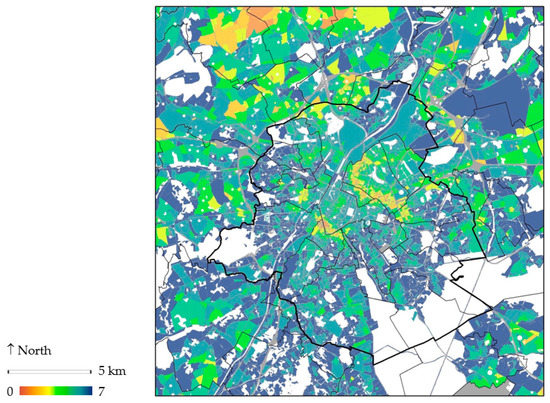
Figure 10.
Number of TFL within range for scenario SUPP.

Figure 11.
Number of TFL within range for scenario FULL. 0  7.
7.
7.
Figure 12 depicts the population share per proximity score (the amount of different TFL within reach). Since proximity to residential GS and play GS are not considered in the scenarios, the proximity score can be maximum 5 instead of 7. Ideally, the population share is 100% for proximity score 5 and 0% for 0–4. The existing state CURR shows a large margin for improvement in the range 4–5. Around 1/5th of the population has a proximity score of only 1–2, and nearly 1/10th of the population has no neighbourhood GS or larger within reach. Whereas the BASE scenario gives the impression of significant change when observing the maps, in terms of population impact there is only a slight change of around 10% increase for proximity scores 4–5 and around 5% decrease in the proximity scores 0–3. The scenario halves the population with proximity score 0 but leaves about 5% of the population with no neighbourhood GS or larger public GS within reach. The population with proximity scores 0–2 lowers from 30% to 19%; however, it requires the SUPP scenario to make this segment drop below 6%. In this scenario, changes become clear, as the population share with full access to higher-level GS (proximity score 5) reaches 53%, while the population with no access to public GS of neighbourhood level or larger drops to 0%. In the FULL scenario, 78% of the population has a proximity score of 5 and 99% has a score of 3 or higher. The centre–periphery contrast disappears, and the BCR achieves a balanced, high-quality provision of public GS.
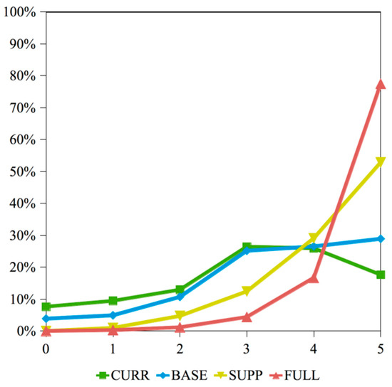
Figure 12.
Share of population that has 1–5 TFL of public green space within range for CURR and scenarios BASE, SUPP, FULL.
As explained before, design interventions for residential GS and play GS have not been tested for the full study area due to the large number of potential interventions. One of the most challenging test areas was selected for a design exercise, based on the lack of such public GS, low income, and high imperviousness. Despite these challenges for the test area, the OGSD that have been identified appeared to be sufficient to cover the lack of these small public GS. The higher-than-normal investment costs related to, for example, developing public intensive green roofs, parks in urban block interiors, or car-free street and boulevard transformations make these OGSD not feasible within the BASE scenario. During the workshop, a discussion about the practical implications of green space development, experts, and designers agreed that these spaces do not only require elaborate spatial design, but also innovation related to the stakeholder process, legislation, and management. Examples are the management and insurance responsibilities for rooftop parks, the controversial aspect of making streets (partly) car-free, the high number of landowners involved for implementing urban block interior parks and the access management, the high number of stakeholders for street transformation, and consultation with fire departments and other emergency services and their willingness to change or co-create guidelines for unprecedented spatial configurations.
3.4. Inequalities in Green Space Proximity under Different Scenarios
Figure 13 shows the spatial distribution of urban blocks located within low versus medium-to-high average incomes for the BCR. The focus is on the BCR only, given its high population density and public GS demand. The selected urban blocks form an almost contiguous area along the canal zone. Urban blocks are split into two categories: those located within the 25% statistical sectors with the lowest average reported income (BOT25), and those located within statistical sectors where the average reported income is higher (TOP75).
Figure 13.
Urban blocks in neighbourhoods with TOP75 (grey) and BOT25 (blue) average incomes; the Brussels Canal is shown in black. No data is shown in scarcely populated statistical sectors (white). Scale: 5 km.
5 km.
In Figure 14, the influence of income on public GS accessibility is shown for the current situation, along with the potential of the three scenarios for improving access to public GS in low-income vs. medium-to-high-income neighbourhoods. For each category, the population percentage with GS of different TFL within reach is shown for the current state (CURR) and for each of the three scenarios (BASE, SUPP, FULL). The lowest TFL residential GS and play GS, for which no interventions are proposed in the scenarios, show an increase in reached population due to the fact that higher TFL are considered as covering the functions of lower TFL if they are within reach [19,25]. In the current state (CURR), metropolitan GS, city GS, and residential GS are the lowest-performing TFL region-wide with, respectively, 42%, 52%, and 55% of the population within reach. However, it is possible to elevate the reach of the five highest TFL to a very high level in the FULL scenario. In CURR, the average accessibility for all TFL for the BOT25 group in terms of fraction of the people reached is about 40% lower than for the TOP75 group (Figure 15), meaning that inhabitants living in the lowest-income neighbourhoods are strongly disadvantaged in terms of public GS access. Access is especially low for the BOT25 group for city and metropolitan GS (Figure 14). The BASE scenario has nearly no impact (3%) in terms of improving people’s access to GS overall. The SUPP scenario, on the other hand, leads to a substantial increase in accessibility for the five highest-level TFL, especially for BOT25 neighbourhoods, where the scenario impact is much higher than for the TOP75 group (Figure 16). In addition, for the FULL scenario the gain is higher for the disadvantaged BOT25 group than for the TOP75 group, restoring the balance for both groups in terms of access to GS for most TFL. Only city green and residential public GS access remains lower for BOT25 than for TOP75 (Figure 16).
Figure 14.
Percentage of population in low- and in medium-to-high-income neighbourhoods (BOT25, TOP75) and in the entire BCR (TOT) having access to each TFL in each scenario.
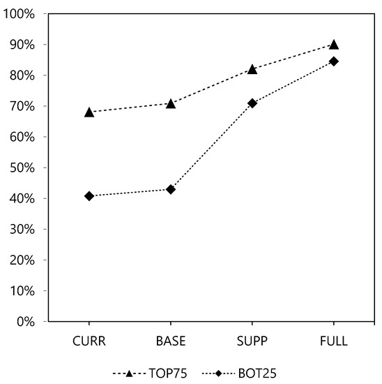
Figure 15.
Average fraction of people reached for all TFL in each scenario for low-income (BOT25) and for medium-to-high-income groups (TOP75).
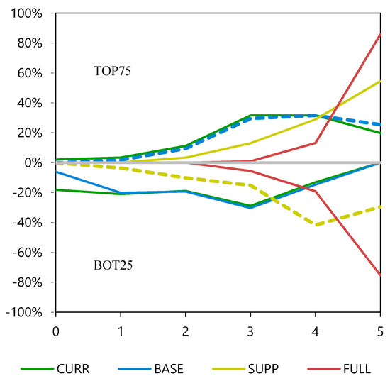
Figure 16.
Population share per proximity score (0–5) for low-income (BOT25) and for medium-to-high-income groups (TOP75).
Figure 16 shows the population share per proximity score per scenario for the five highest-level TFL for both population groups. The disadvantage of the BOT25 group is clearly visible for CURR and for the BASE scenario. The results show a higher FULL scenario potential for the TOP75 group, as well as some similarity of potential between the TOP75-BASE scenario and the BOT25-SUPP scenario. Therefore, in case an equitable public GS development is the priority, public GS development goals and investment levels might be differentiated as such, to generate similar public GS provision for low-income neighbourhoods and medium-to-high-income neighbourhoods.
4. Discussion
The RbD experiment shows the potential of the TFL proximity model that was developed by the authors [25], and its indicators, as a design and decision making tool. It allows the identification of problem areas. The output of the model helps in determining possible locations and interventions and allows measurement of the impact of proposed solutions on citizens’ access to public GS. Design exercises have shown the possibility for the BCR of moving away from a public GS status quo and reducing inequalities in public GS provision. The question of whether the solutions proposed are financially realistic is not addressed in this paper; however, the relation between approximated level of investment, its effect, and how to prioritise has been explored by means of scenarios.
Scenario definition in this study was limited to larger-size green spaces, from metropolitan to neighbourhood green. In further studies, the feasibility and typologies of OGSD at the level of residential and play green can be further elaborated, though exploration of RbD interventions in a focus area has shown the potential of a high level of GS provision for small public green spaces despite high built-up densities. Different types of OGSD can be defined for each TFL, corresponding to a range of interventions, sometimes unique to the TFL, sometimes spanning over several TFL. Identifying these types can contribute to the streamlining of identifying suitable locations for their realisation in the form of actual projects.
The three scenarios developed for the BCR show the negligible contribution of low-investment developments in the BASE scenario and the necessity of multidisciplinary, higher-investment GS development on challenging sites (SUPP/FULL scenarios). With regards to scenario implementation, mainly the interaction with traffic infrastructure poses an implementation challenge; however, it can also act as a catalyst to move towards more sustainable mobility. The design exercises point to the necessity of infrastructure adaptations that reorganise or lessen traffic flow and of the acquisition of empty (parts of) residential plots in favour of the GS. In accordance with other studies, design exercises showed a range of possibilities in adaptive use of sub-optimal or vacant urban infrastructure, brownfields, and gap sites [39,44,45], or gap space on occupied sites, as well as in covering of rail corridors and development of intensive green roofs adjacent to public green spaces.
Monitoring evolutions in the proximity score for different scenarios, thereby differentiating between various income groups (Figure 14), may be especially useful for setting policy priorities and for monitoring the balance between income groups in terms of access to a range of GS with different functionalities. However, there is a paradoxical aspect to the development of equity in access to GS. The inhabitants of neighbourhoods that are made healthier and more attractive through new or improved GS development are often confronted with gentrification caused by increasing property value [33,46], a process commonly referred to as environmental gentrification [47]. As such, policies and interventions can miss the intended receivers of benefits. Decision-makers, planners, and designers should therefore make cities and neighbourhoods ‘just green enough’ [33]. GS development has to be planned in an orchestrated way throughout the city for minimal gentrification effects, or GS development must be paired with strategies that prevent negative gentrification impacts, for example, careful urban renewal (behutsame Statdterneuerung) for the preservation of the social composition of the population [48]. Strategies include: an encouragement of citizens’ participation, transfer of land to public re-developers (right of first purchase and first refusal for public authorities), and instalment of rent caps and minimum lease terms. Another approach could be to improve proximity scores throughout the area without strongly affecting the relative ranking of the current situation, related to the ‘just green enough’ strategy [33]. The gradual implementation of the BASE and SUPP scenarios in the BCR largely allow maintaining this relative ranking. To assess GS availability and the effect of future developments, scenario simulation is a key element in decision-making and design.
The sustainable regional development plan [49,50] points out the need for strategic and holistic plans for the BCR that comprise the entire region [51]. The realization of such plans can be supported by the findings of this study, as well as by the tool that was presented. Effective green space planning is of crucial importance, especially in already compact cities [39] due to the many constraints, and particularly, the scarcity of space [52,53,54].
As partly demonstrated by the design exercises, public green space planning requires more information than is available on ecosystem services and social valuation [55]. Citizen input can be of key importance for the collection of this information. Over the years, the research and planning community has experimented with Participatory GIS (PGIS), also referred to as Public Participation GIS (PPGIS). PPGIS is a framework that allows the combination of expert knowledge and public input [56] by means of map-based surveys or geo-questionnaires [57,58]. Whereas participatory mapping was the ‘analogue’ procedure, PPGIS is digital [58]. This tool can help, for example, to target conflict areas, identify user preferences, improve the accuracy of expert-based assessments, enhance multifunctionality assessment, and especially, ensure social inclusion in the process. [55]. However, PPGIS cannot substitute debate over planning alternatives [55,59,60].
Whereas most proposals or experiments with PPGIS focus on the collection of information about existing GS, the potential for PPGIS is different in this case. The public can be consulted for two action points in the methodology: identifying OGSD and defining scenarios. For defining OGSD, an interactive mapping tool can be created, where users can delineate OGSD, identify the type of interventions related to it (e.g., land acquisition, deviating traffic), and receive real-time feedback about two indicators: to which socio-economic subgroups the GS caters, and how many people have the GS within reach (and no other GS of the same functional level), per GS area. Both are impact indicators of a specific type. For the defining of the scenarios, users can select either their own delineated spaces or spaces delineated by other users. These PPGIS interactions also have the potential to take form as a game, whereby the goal is to achieve maximum impact with limited resources, in a fair and equitable way. Studies have found that the combination of decision support tools and gaming procedures can support agenda setting and foster a shared understanding of challenges and potential solutions in the field of sustainable urban renewal [61].
While this study focuses on GS proximity, recent work [41] has demonstrated that inherent aspects of GS quality, such as naturalness and spaciousness, and how these qualities are valued by GS users, may be predicted from land-cover-based variables such as the fraction of dense/woody vegetation, herbaceous vegetation, impervious area, and water within GS, as well as from variables indicating biological value. By including these types of variables in design exercises, the methodology proposed in this study may be extended by incorporating aspects of GS quality in the scenario modelling. Since quality indicators partly require use-related ratings [41], the common use of PPGIS (data collection for existing GS) can be applied in this case.
5. Conclusions
Collaborative design was mobilised to explore the potential for GS development in Brussels and its surroundings. Analysis of the current state and of three GS development scenarios corresponding to different investment levels were conducted with the proximity model developed by Stessens, Khan, Huysmans and Canters [25], which enables spatially explicit analysis of citizen’s access to green spaces of different sizes, fulfilling different needs. Impact analysis showed that inhabitants of low-income neighbourhoods have limited access to larger green spaces. Actions to provide low-income neighbourhoods with a good accessibility to public green spaces require creative solutions. These are spatial solutions, dealing with property, management, and investments that go beyond the cost of regular GS development. Legal frameworks to designate urban GS are essential for reaching intended goals [39].
The main objective of this paper was to identify possible GS development scenarios for the Brussels’ study area and to assess how these scenarios benefit the population of Brussels as a whole, as well as different socio-economic segments of the population. The proposed method generated an unprecedented view on the practical feasibility of providing a high degree of GS proximity for the inhabitants of the Brussels-Capital Region and its surroundings. Whereas ordinary GS development would benefit both poor and rich neighbourhoods to a very low degree, medium to high investments will mainly advance the poorer neighbourhoods and bring them to a comparable level of GS proximity as the wealthier areas. The socio-economic bias of benefits by urban GS provision in the form of recreational nature, which is described in literature and proven for the case of Brussels, can be resolved. A caution towards negative effects of gentrification is advised, however.
The creation of scenarios involved collaborative workshops where: (i) the GS proximity indicators developed in Stessens, Khan, Huysmans and Canters [25], along with the proposed supplementary maps were deemed very useful for identifying problem areas and locations and proposing solutions; (ii) the process of collaborative RbD has proven to be an appropriate method for the same goal, especially for discussing the feasibility of solutions, and; (iii) the necessity of the combination of various indicator maps and supplementary maps has confirmed the effectiveness of the graphic overlay method, commonly used in landscape design. The creation of scenarios can benefit from additional data regarding the financial impact of proposed GS developments; however, the great relative investment scales allow for a rough classification from practical experience. A coarse classification of OGSD proved to be sufficient to formulate scenarios. The analysis of interventions needed for the realization for each OGSD resulted in a classification according to recurrent types per TFL. This is valuable information for further analysis, as they can streamline the process of finding OGSD in new cases.
The research is novel in its combination of three aspects: (i) high-resolution proximity indicators, calculated at the urban block level, using path network distances; (ii) in-depth collaborative and individual RbD exercises (162 OGSD with estimated investment class); and (iii) scenario impact in relation to socio-economic indicators. Few academic studies have performed similar in-depth analyses of concrete situations with the support of GIS models and collaborative RbD. This is a method with significant potential for future studies and application potential for policy documents and spatial development plans.
Future research can be conducted on the mapping of aspects of inherent GS quality (quietness, naturalness, historical/cultural value), not for existing spaces, but for the remaining open space where OGSD can be located. This would be a valuable data layer to be involved in defining scenarios. The whole methodology can be streamlined by creating a user interface with real-time feedback on consequences of choosing certain locations of OGSD, for example, demographic impact, investment scale, water buffering potential, ecological network, or inherent quality aspects.
Author Contributions
Conceptualization, P.S., A.Z.K. and F.C.; methodology, P.S., A.Z.K. and F.C.; software, P.S.; validation, P.S.; formal analysis:, P.S.; investigation, P.S.; resources, P.S., A.Z.K., F.C., and Marijke Huysmans; data curation, P.S.; writing—original draft preparation, P.S., A.Z.K. and F.C.; writing—review and editing, P.S., A.Z.K. and F.C.; visualization, P.S.; supervision, A.Z.K. and F.C.; project administration, A.Z.K. and F.C.; funding acquisition, P.S., A.Z.K. and F.C. All authors have read and agreed to the published version of the manuscript.
Funding
This work was supported by the Brussels-Capital Region via the Innoviris Prospective Research grant, number 2014-PRFB-1.
Institutional Review Board Statement
Not applicable.
Informed Consent Statement
Not applicable.
Data Availability Statement
The data related to this study can be requested from the authors via the correspondence address.
Acknowledgments
The authors thank Sebastiaan Willemen for his contributions through preliminary design exploration of green space development opportunities in his master’s thesis “Green Space Provision in The Brussels Metropolitan Region—Analysis and Research by Design of Urban Landscape Infrastructure Towards an Improved Urban Environmental Quality”.
Conflicts of Interest
The authors have no conflict of interest to declare.
Appendix A
Table A1.
Listing of identified opportunities for green space development and involved strategies 1/5 (continued on next page).
Table A1.
Listing of identified opportunities for green space development and involved strategies 1/5 (continued on next page).
| Type–Name/Count | Tunnel Construction | Infrastructure Works | Compulsory Res. Real Estate Acquisition | Compulsory Industr. Real Estate Acquisition | Changing Public Facilities | Agricultural Land Acquisition | Noise Barriers | Constructing Paths and Routes | Number of Strategies–59 | Number of Strategies for Metropolitan GS–9 | Number of Strategies for City GS–8 | Number of Strategies for District GS–13 | Number of Strategies for Quarter GS–9 | Number of Strategies for Neighborhood GS–21 | Number of Strategies for Play GS–5 | Number of Strategies for Residential GS–8 | Intra-Urban Metropolitan GS | Peri-Urban Metripolitan GS | Rural Metropolitan GS | Valley Parks | Agriculture Reconversions to Valley Parks | Agriculture Reconversions | Urban Space Optimization | Functional Level Scaling | Inner City District GS Optimization | Inner City Continuous Spaces | Peri-urban District GS Development | De-Privatizing Domains | Rural Disctrict GS | District GS Development in Tributary Valleys | Expanding Existing Parks | Conversion/Reorganization | Green Roof on Commercial Buildings | Converting Farmland to Park Space | Railroad Optimization | Private Gardens to Park Space | Mega-Block | De-Privatizing Estates | Public Space Redevelopment of Housing Blocks | Reorganizing Sports Fields | Brownfield Development | Rural Neighborhood GS Development | |
|---|---|---|---|---|---|---|---|---|---|---|---|---|---|---|---|---|---|---|---|---|---|---|---|---|---|---|---|---|---|---|---|---|---|---|---|---|---|---|---|---|---|---|---|
| TFL/N° | Σ | M | C | D | Q | N | P | R | M | M | M | C | C | C | C | D | D | D | D | D | D | D | Q | Q | Q | Q | N | N | N | N | N | N | N | N | |||||||||
| High investment class–FULL scenario | x | x | x | x | |||||||||||||||||||||||||||||||||||||||
| Middle investment class–SUPP scenario | x | x | x | x | x | x | x | x | x | x | |||||||||||||||||||||||||||||||||
| Low investment class–BASE scenario | x | x | x | x | x | x | x | x | x | x | x | x | x | x | x | x | |||||||||||||||||||||||||||
| 1 | Developing wetlands in valley bottom | 12 | 4 | 5 | 2 | 1 | 0 | 0 | 0 | x | x | x | x | x | |||||||||||||||||||||||||||||
| 2 | Developing a blue-green network | 20 | 9 | 6 | 2 | 2 | 0 | 0 | 0 | x | x | x | x | x | x | ||||||||||||||||||||||||||||
| 3 | Deploying walking and cycling trajectories | x | 21 | 9 | 8 | 0 | 0 | 0 | 2 | 1 | x | x | x | x | x | x | |||||||||||||||||||||||||||
| 4 | Converting agricultural fields to park space with small scale agricultural character | x | 59 | 9 | 6 | 13 | 9 | 21 | 0 | 0 | x | x | x | x | x | x | x | x | x | ||||||||||||||||||||||||
| 5 | Developing green areas around upstream tributaries | 11 | 5 | 3 | 3 | 0 | 0 | 0 | 0 | x | x | x | |||||||||||||||||||||||||||||||
| 6 | Cutting local road | 30 | 7 | 5 | 6 | 8 | 0 | 2 | 1 | x | x | x | x | x | x | x | x | ||||||||||||||||||||||||||
| 7 | Connecting existing public green spaces | 29 | 8 | 7 | 6 | 7 | 0 | 0 | 0 | x | x | x | x | x | x | x | |||||||||||||||||||||||||||
| 8 | Halting housing development | 9 | 5 | 3 | 0 | 0 | 0 | 0 | 0 | x | x | ||||||||||||||||||||||||||||||||
| 9 | Reversing housing development | x | 7 | 5 | 2 | 0 | 0 | 0 | 0 | 0 | x | ||||||||||||||||||||||||||||||||
| 10 | Noise shielding | x | 19 | 6 | 2 | 5 | 4 | 2 | 0 | 0 | x | x | x | x | |||||||||||||||||||||||||||||
| 11 | Integrating protected landscapes | 11 | 5 | 1 | 4 | 0 | 0 | 0 | 0 | x | x | x | x | x | |||||||||||||||||||||||||||||
| 12 | Integrating estates | 10 | 0 | 1 | 1 | 3 | 5 | 0 | 0 | x | x | ||||||||||||||||||||||||||||||||
| 13 | Connecting separate parts over 2 × 2-lane road | x | 4 | 2 | 1 | 1 | 0 | 0 | 0 | 0 | x | ||||||||||||||||||||||||||||||||
| 14 | Connecting to railway station | 11 | 4 | 2 | 1 | 2 | 0 | 1 | 1 | x | x | ||||||||||||||||||||||||||||||||
| 15 | Covering open railroad trenches | x | 9 | 0 | 2 | 2 | 0 | 5 | 0 | 0 | x | x | |||||||||||||||||||||||||||||||
| 16 | Connecting to tram station | 15 | 2 | 3 | 5 | 5 | 0 | 0 | 0 | x | x | x | x | ||||||||||||||||||||||||||||||
| 17 | Extending park over local road up to sidewalk | 4 | 0 | 0 | 3 | 0 | 0 | 1 | 0 | x | |||||||||||||||||||||||||||||||||
| 18 | Re-routing roads and traffic around or away from park | x | 8 | 0 | 0 | 4 | 1 | 2 | 1 | 0 | x | ||||||||||||||||||||||||||||||||
| 19 | Putting through traffic underground/covering open tunnels | x | 9 | 0 | 0 | 5 | 3 | 1 | 0 | 0 | x | x | |||||||||||||||||||||||||||||||
| 20 | Transforming urban boulevard to park strip | x | 4 | 0 | 0 | 0 | 2 | 1 | 0 | 1 | |||||||||||||||||||||||||||||||||
| 21 | Greening tram beds crossing the GS | 2 | 0 | 0 | 2 | 0 | 0 | 0 | 0 | x | |||||||||||||||||||||||||||||||||
| 22 | Cutting park drives for cars | 2 | 0 | 1 | 1 | 0 | 0 | 0 | 0 | x | |||||||||||||||||||||||||||||||||
| 23 | Connecting to metro station | 7 | 1 | 0 | 2 | 4 | 0 | 0 | 0 | x | x | ||||||||||||||||||||||||||||||||
| 24 | Re-integrating derelict/brownfield / unused land | 7 | 1 | 0 | 2 | 1 | 2 | 0 | 1 | x | x | ||||||||||||||||||||||||||||||||
| 25 | Connecting to highway | 4 | 3 | 1 | 0 | 0 | 0 | 0 | 0 | ||||||||||||||||||||||||||||||||||
| 26 | Moving logistic activities and light industry | x | 8 | 1 | 1 | 1 | 1 | 3 | 0 | 1 | |||||||||||||||||||||||||||||||||
| 27 | Integrating nature reserves | 2 | 1 | 1 | 0 | 0 | 0 | 0 | 0 | ||||||||||||||||||||||||||||||||||
| 28 | Connecting separate parts over highway | x | 2 | 2 | 0 | 0 | 0 | 0 | 0 | 0 | |||||||||||||||||||||||||||||||||
| 29 | Connecting over causeway | x | 3 | 2 | 0 | 0 | 1 | 0 | 0 | 0 | |||||||||||||||||||||||||||||||||
| 30 | Connecting over/under local road | x | 7 | 1 | 1 | 2 | 2 | 1 | 0 | 0 | |||||||||||||||||||||||||||||||||
| 31 | Visual shielding | 4 | 1 | 0 | 2 | 0 | 1 | 0 | 0 | ||||||||||||||||||||||||||||||||||
| 32 | Making fenced off grounds accessible integrating sports grounds | 5 | 0 | 1 | 2 | 1 | 1 | 0 | 0 | ||||||||||||||||||||||||||||||||||
| 33 | Renegociating industrial land for shared use | 4 | 1 | 0 | 0 | 0 | 0 | 3 | 0 | ||||||||||||||||||||||||||||||||||
| 34 | Connecting nearby housing projects with parkspace | 4 | 0 | 0 | 2 | 0 | 0 | 0 | 2 | ||||||||||||||||||||||||||||||||||
| 35 | Re-designing ground floor and terrains of 60’s housing blocks | x | 8 | 0 | 0 | 1 | 0 | 6 | 0 | 1 | x | ||||||||||||||||||||||||||||||||
| 36 | Developing real estate around GS | 5 | 0 | 0 | 0 | 5 | 0 | 0 | 0 | x | |||||||||||||||||||||||||||||||||
| 37 | Reorganizing open air sports facilities | x | 10 | 0 | 0 | 0 | 3 | 4 | 2 | 1 | x | x | |||||||||||||||||||||||||||||||
| 38 | Opening up impervious surfaces | 20 | 0 | 0 | 2 | 5 | 0 | 5 | 8 | x | x | ||||||||||||||||||||||||||||||||
| 39 | Rooftop park extension on commercial buildings | 1 | 0 | 0 | 0 | 1 | 0 | 0 | 0 | x | |||||||||||||||||||||||||||||||||
| 40 | Rooftop park extension on public buildings | x | 3 | 0 | 0 | 0 | 2 | 0 | 0 | 1 | x | ||||||||||||||||||||||||||||||||
| 41 | Creating passages in-between buildings | 5 | 0 | 0 | 0 | 2 | 0 | 0 | 3 | ||||||||||||||||||||||||||||||||||
| 42 | Mega-roundabout | x | 1 | 0 | 1 | 0 | 0 | 0 | 0 | 0 | |||||||||||||||||||||||||||||||||
| 43 | Mega-block | x | 4 | 0 | 0 | 0 | 0 | 4 | 0 | 0 | x | ||||||||||||||||||||||||||||||||
| 44 | Part of private garden to parkspace | x | 17 | 0 | 0 | 2 | 2 | 8 | 0 | 5 | x | ||||||||||||||||||||||||||||||||
| 45 | GS as part of strategic site redevelopment | 2 | 0 | 0 | 0 | 1 | 0 | 0 | 1 | ||||||||||||||||||||||||||||||||||
| 46 | Connecting over water body | 2 | 1 | 0 | 0 | 0 | 0 | 0 | 0 | ||||||||||||||||||||||||||||||||||
| 47 | GS in shared use with public services | 3 | 0 | 0 | 0 | 0 | 2 | 0 | 0 | ||||||||||||||||||||||||||||||||||
| 48 | Transforming local road into GS | 13 | 0 | 0 | 0 | 1 | 8 | 2 | 2 | ||||||||||||||||||||||||||||||||||
| 49 | Transformation public space into park | 7 | 0 | 0 | 0 | 0 | 3 | 3 | 1 | ||||||||||||||||||||||||||||||||||
| 50 | Rooftop park on top of industrial building | 6 | 0 | 0 | 0 | 0 | 1 | 4 | 1 | ||||||||||||||||||||||||||||||||||
| 51 | Reversing commercial building | 2 | 0 | 0 | 0 | 0 | 0 | 2 | 0 | ||||||||||||||||||||||||||||||||||
| 52 | Demolishing existing building for creation of GS | 2 | 0 | 0 | 0 | 0 | 1 | 0 | 1 | ||||||||||||||||||||||||||||||||||
| 53 | Converting parking space into GS | 4 | 0 | 0 | 0 | 0 | 2 | 1 | 1 | ||||||||||||||||||||||||||||||||||
| 54 | Cutting parking spaces | 7 | 0 | 0 | 0 | 1 | 4 | 0 | 2 | ||||||||||||||||||||||||||||||||||
| 55 | Activation of unused lawn | 9 | 0 | 0 | 0 | 1 | 5 | 0 | 3 |
Table A2.
Listing of identified opportunities for green space development and involved strategies 2/5 (continued on next page).
Table A2.
Listing of identified opportunities for green space development and involved strategies 2/5 (continued on next page).
| Type–Name/Count | Intra-Urban MGS—Koning Boudewijnpark, Moeras van Ganshoren, ... | Intra-Urban MGS—Zuidelijke Zennevallei | Peri-Urban MGS–Perk | Rural MGS–Asse | Rural MGS–Neerpede | Rural MGS–Groenenberg | Rural MGS - Kravaalbos (Liedekerke) | Rural MGS–Hertigembos | Rural MGS–Plutsingen | Rural MGS–Kanaal | Valley Parks–Bollebeek | Valley Parks–Hagaard | Agreculture Reconversion to Valley Parks—Merchtem | Agreculture Reconversion to Valley Parks—Sint-Martens Bodegem Park | Agreculture Reconversion to Valley Parks–Sint-Pieters-Leeuw | Agriculture Reconversions–NATO | Agriculture Reconversions–Moorsel | Urban space Optimization–Scheutbos | Un-Fragmented Park Space–Terkamerenbos | Urban Space Optimization–Josaphat | Functional Level Scaling—Albertpark, Marie-Josépark, Weststation | Functional Level Scaling—Tour&Taxis | Inner City District GS Optimization–Jubelpark | Inner City District GS Optimization–Koekelberg | Inner City District GS Optimization–Warandepark | Continuous Inner City Spaces–Vijvers van Elsene, Abdij | Continuous Inner City Spaces—Ste. Catherine | Peri-Urban DGS Development–Zellik | Peri-Urban DGS Development–Diegem | Peri-Urban DGS Development–Machelen | Peri-Urban DGS Development–Faubourg | Peri-Urban DGS Development–Zaventem | De-Privatizing Domains–Kasteeel ter Meeren | Rural DGS–De Hoek | Rural DGS–La hulpe | Valley Bottom DGS–La hulpe Vallée | Highway Rooftop Park–R0 Afrit 1-2 | Inner City DGS Optimization–Visserij | Rural DGS Development | Rural DGS Development | Rural DGS Development | Rural DGS Development | Rural DGS Development | Rural DGS Development | |
|---|---|---|---|---|---|---|---|---|---|---|---|---|---|---|---|---|---|---|---|---|---|---|---|---|---|---|---|---|---|---|---|---|---|---|---|---|---|---|---|---|---|---|---|---|---|
| TFL/N° | M1 | M9 | M4 | M5 | M2 | M3 | M6 | M7 | M8 | M10 | C1 | C2 | C4 | C5 | C6 | C8 | C9 | C10 | C11 | C12 | D1 | D6 | D2 | D3 | D5 | D7 | D18 | D8 | D10 | D11 | D12 | D13 | D14 | D15 | D16 | D17 | D9 | D19 | D20 | D22 | D23 | D24 | D28 | D29 | |
| High investment class–FULL scenario | x | x | x | x | x | x | x | ||||||||||||||||||||||||||||||||||||||
| Middle investment class–SUPP scenario | x | x | x | x | x | x | x | x | x | x | x | x | x | x | x | ||||||||||||||||||||||||||||||
| Low investment class–BASE scenario | x | x | x | x | x | x | x | x | x | x | x | x | x | x | x | x | x | x | x | x | x | x | |||||||||||||||||||||||
| 1 | Developing wetlands in valley bottom | x | x | x | x | x | x | x | x | x | x | x | |||||||||||||||||||||||||||||||||
| 2 | Developing a blue-green network | x | x | x | x | x | x | x | x | x | x | x | x | x | x | x | x | x | x | ||||||||||||||||||||||||||
| 3 | Deploying walking and cycling trajectories | x | x | x | x | x | x | x | x | x | x | x | x | x | x | x | x | x | x | ||||||||||||||||||||||||||
| 4 | Converting agricultural fields to park space with small scale agricultural character | x | x | x | x | x | x | x | x | x | x | x | x | x | x | x | x | x | x | x | x | x | x | x | x | x | x | x | x | x | |||||||||||||||
| 5 | Developing green areas around upstream tributaries | x | x | x | x | x | x | x | x | x | x | x | |||||||||||||||||||||||||||||||||
| 6 | Cutting local road | x | x | x | x | x | x | x | x | x | x | x | x | x | x | x | x | x | x | x | |||||||||||||||||||||||||
| 7 | Connecting existing public green spaces | x | x | x | x | x | x | x | x | x | x | x | x | x | x | x | x | x | x | x | x | x | x | ||||||||||||||||||||||
| 8 | Halting housing development | x | x | x | x | x | x | x | x | x | |||||||||||||||||||||||||||||||||||
| 9 | Reversing housing development | x | x | x | x | x | x | x | |||||||||||||||||||||||||||||||||||||
| 10 | Noise shielding | x | x | x | x | x | x | x | x | x | x | x | x | x | |||||||||||||||||||||||||||||||
| 11 | Integrating protected landscapes | x | x | x | x | x | x | x | x | x | x | x | |||||||||||||||||||||||||||||||||
| 12 | Integrating estates | x | x | ||||||||||||||||||||||||||||||||||||||||||
| 13 | Connecting separate parts over 2 × 2-lane road | x | x | x | x | ||||||||||||||||||||||||||||||||||||||||
| 14 | Connecting to railway station | x | x | x | x | x | x | x | |||||||||||||||||||||||||||||||||||||
| 15 | Covering open railroad trenches | x | x | x | x | ||||||||||||||||||||||||||||||||||||||||
| 16 | Connecting to tram station | x | x | x | x | x | x | x | x | x | x | ||||||||||||||||||||||||||||||||||
| 17 | Extending park over local road up to sidewalk | x | x | x | |||||||||||||||||||||||||||||||||||||||||
| 18 | Re-routing roads and traffic around or away from park | x | x | x | x | ||||||||||||||||||||||||||||||||||||||||
| 19 | Putting through traffic underground/covering open tunnels | x | x | x | x | x | |||||||||||||||||||||||||||||||||||||||
| 20 | Transforming urban boulevard to park strip | ||||||||||||||||||||||||||||||||||||||||||||
| 21 | Greening tram beds crossing the GS | x | x | ||||||||||||||||||||||||||||||||||||||||||
| 22 | Cutting park drives for cars | x | x | ||||||||||||||||||||||||||||||||||||||||||
| 23 | Connecting to metro station | x | x | x | |||||||||||||||||||||||||||||||||||||||||
| 24 | Re-integrating derelict/brownfield/unused land | x | x | x | |||||||||||||||||||||||||||||||||||||||||
| 25 | Connecting to highway | x | x | x | x | ||||||||||||||||||||||||||||||||||||||||
| 26 | Moving logistic activities and light industry | x | x | x | |||||||||||||||||||||||||||||||||||||||||
| 27 | Integrating nature reserves | x | x | ||||||||||||||||||||||||||||||||||||||||||
| 28 | Connecting separate parts over highway | x | x | ||||||||||||||||||||||||||||||||||||||||||
| 29 | Connecting over causeway | x | x | ||||||||||||||||||||||||||||||||||||||||||
| 30 | Connecting over/under local road | x | x | x | x | ||||||||||||||||||||||||||||||||||||||||
| 31 | Visual shielding | x | x | x | |||||||||||||||||||||||||||||||||||||||||
| 32 | Making fenced off grounds accessible integrating sports grounds | x | x | x | |||||||||||||||||||||||||||||||||||||||||
| 33 | Renegociating industrial land for shared use | x | |||||||||||||||||||||||||||||||||||||||||||
| 34 | Connecting nearby housing projects with parkspace | x | x | ||||||||||||||||||||||||||||||||||||||||||
| 35 | Re-designing ground floor and terrains of 60’s housing blocks | x | |||||||||||||||||||||||||||||||||||||||||||
| 36 | Developing real estate around GS | ||||||||||||||||||||||||||||||||||||||||||||
| 37 | Reorganizing open air sports facilities | ||||||||||||||||||||||||||||||||||||||||||||
| 38 | Opening up impervious surfaces | x | x | ||||||||||||||||||||||||||||||||||||||||||
| 39 | Rooftop park extension on commercial buildings | ||||||||||||||||||||||||||||||||||||||||||||
| 40 | Rooftop park extension on public buildings | ||||||||||||||||||||||||||||||||||||||||||||
| 41 | Creating passages in-between buildings | ||||||||||||||||||||||||||||||||||||||||||||
| 42 | Mega-roundabout | x | |||||||||||||||||||||||||||||||||||||||||||
| 43 | Mega-block | ||||||||||||||||||||||||||||||||||||||||||||
| 44 | Part of private garden to parkspace | x | x | ||||||||||||||||||||||||||||||||||||||||||
| 45 | GS as part of strategic site redevelopment | ||||||||||||||||||||||||||||||||||||||||||||
| 46 | Connecting over water body | x | x | ||||||||||||||||||||||||||||||||||||||||||
| 47 | GS in shared use with public services | ||||||||||||||||||||||||||||||||||||||||||||
| 48 | Transforming local road into GS | ||||||||||||||||||||||||||||||||||||||||||||
| 49 | Transformation public space into park | ||||||||||||||||||||||||||||||||||||||||||||
| 50 | Rooftop park on top of industrial building | ||||||||||||||||||||||||||||||||||||||||||||
| 51 | Reversing commercial building | ||||||||||||||||||||||||||||||||||||||||||||
| 52 | Demolishing existing building for creation of GS | ||||||||||||||||||||||||||||||||||||||||||||
| 53 | Converting parking space into GS | ||||||||||||||||||||||||||||||||||||||||||||
| 54 | Cutting parking spaces | ||||||||||||||||||||||||||||||||||||||||||||
| 55 | Activation of unused lawn |
Table A3.
Listing of identified opportunities for green space development and involved strategies 3/5 (continued on next page).
Table A3.
Listing of identified opportunities for green space development and involved strategies 3/5 (continued on next page).
| Type–Name/Count | Opening up Hardscape–Abbattoir | Expanding Park–Kruidtuin | Inner city District GS Optimization–Hallepoort | Boulevard to Parkstrip–Montgomery | Expanding Park–Haren | Complex Node–Ninoofsepoort | Conversion of Sport and Industrial Land–Schaarbeek Kerkhof | Reorganization of Sports–Machelen | Sports Facilities to Green roof–Zaventem | Commercial Green Roof–Witte Cité | Commercial Green Roof–Hanssenpark | Prison to Park–Ducpétiaux | Farmland to Park–Diegem | Farmland to Park–Nossegem | Farmland to Park–Smeiberg | Farmland to Park–Hoge Heide | Farmland to Park–Terrestpark | Farmland to Park–Drogenberg | Opening up Valley Forest–Hagaard | GS as Part of Development–VRT | Railroad Optimization | Railroad Optimization | Railroad Optimization | Railroad Optimization | Railroad Optimization | Private Gardens to Parkspace | Private Gardens to Parkspace | Private Gardens to Parkspace | Private Gardens to Parkspace | Private Gardens to Parkspace | Private Gardens to Parkspace | Mega-Block | Mega-Block | Mega-Block | Mega-Block | Boulevard to Parkstrip | Brownfield Development | De-Privatizing Estates | De-Privatizing Estates | |
|---|---|---|---|---|---|---|---|---|---|---|---|---|---|---|---|---|---|---|---|---|---|---|---|---|---|---|---|---|---|---|---|---|---|---|---|---|---|---|---|---|
| TFL/N° | Q1 | Q2 | Q20 | Q5 | Q7 | Q3 | Q6 | Q10 | Q11 | Q9 | Q13 | Q4 | Q8 | Q12 | Q14 | Q15 | Q16 | Q18 | Q17 | Q19 | N2 | N52 | N53 | N55 | N56 | N22 | N44 | N48 | N50 | N51 | N14 | N3 | N5 | N6 | N57 | N1 | N7 | N9 | N11 | |
| High investment class–FULL scenario | x | x | x | x | x | |||||||||||||||||||||||||||||||||||
| Middle investment class–SUPP scenario | x | x | x | x | x | x | x | x | x | x | x | x | x | x | x | x | x | x | x | |||||||||||||||||||||
| Low investment class–BASE scenario | x | x | x | x | x | x | x | x | x | x | x | x | x | x | x | |||||||||||||||||||||||||
| 1 | Developing wetlands in valley bottom | x | ||||||||||||||||||||||||||||||||||||||
| 2 | Developing a blue-green network | x | x | |||||||||||||||||||||||||||||||||||||
| 3 | Deploying walking and cycling trajectories | |||||||||||||||||||||||||||||||||||||||
| 4 | Converting agricultural fields to park space with small scale agricultural character | x | x | x | x | x | x | x | x | x | ||||||||||||||||||||||||||||||
| 5 | Developing green areas around upstream tributaries | |||||||||||||||||||||||||||||||||||||||
| 6 | Cutting local road | x | x | x | x | x | x | x | x | |||||||||||||||||||||||||||||||
| 7 | Connecting existing public green spaces | x | x | x | x | x | x | x | ||||||||||||||||||||||||||||||||
| 8 | Halting housing development | |||||||||||||||||||||||||||||||||||||||
| 9 | Reversing housing development | |||||||||||||||||||||||||||||||||||||||
| 10 | Noise shielding | x | x | x | x | x | x | |||||||||||||||||||||||||||||||||
| 11 | Integrating protected landscapes | |||||||||||||||||||||||||||||||||||||||
| 12 | Integrating estates | x | x | x | x | x | x | x | ||||||||||||||||||||||||||||||||
| 13 | Connecting separate parts over 2 × 2-lane road | |||||||||||||||||||||||||||||||||||||||
| 14 | Connecting to railway station | x | x | |||||||||||||||||||||||||||||||||||||
| 15 | Covering open railroad trenches | x | x | x | x | x | ||||||||||||||||||||||||||||||||||
| 16 | Connecting to tram station | x | x | x | x | x | ||||||||||||||||||||||||||||||||||
| 17 | Extending park over local road up to sidewalk | |||||||||||||||||||||||||||||||||||||||
| 18 | Re-routing roads and traffic around or away from park | x | x | |||||||||||||||||||||||||||||||||||||
| 19 | Putting through traffic underground/covering open tunnels | x | x | x | x | |||||||||||||||||||||||||||||||||||
| 20 | Transforming urban boulevard to park strip | x | x | x | ||||||||||||||||||||||||||||||||||||
| 21 | Greening tram beds crossing the GS | |||||||||||||||||||||||||||||||||||||||
| 22 | Cutting park drives for cars | |||||||||||||||||||||||||||||||||||||||
| 23 | Connecting to metro station | x | x | x | x | |||||||||||||||||||||||||||||||||||
| 24 | Re-integrating derelict/brownfield/unused land | x | x | |||||||||||||||||||||||||||||||||||||
| 25 | Connecting to highway | |||||||||||||||||||||||||||||||||||||||
| 26 | Moving logistic activities and light industry | x | x | x | ||||||||||||||||||||||||||||||||||||
| 27 | Integrating nature reserves | |||||||||||||||||||||||||||||||||||||||
| 28 | Connecting separate parts over highway | |||||||||||||||||||||||||||||||||||||||
| 29 | Connecting over causeway | x | ||||||||||||||||||||||||||||||||||||||
| 30 | Connecting over/under local road | x | x | |||||||||||||||||||||||||||||||||||||
| 31 | Visual shielding | x | ||||||||||||||||||||||||||||||||||||||
| 32 | Making fenced off grounds accessible integrating sports grounds | x | x | |||||||||||||||||||||||||||||||||||||
| 33 | Renegociating industrial land for shared use | |||||||||||||||||||||||||||||||||||||||
| 34 | Connecting nearby housing projects with parkspace | |||||||||||||||||||||||||||||||||||||||
| 35 | Re-designing ground floor and terrains of 60’s housing blocks | |||||||||||||||||||||||||||||||||||||||
| 36 | Developing real estate around GS | x | x | x | x | x | ||||||||||||||||||||||||||||||||||
| 37 | Reorganizing open air sports facilities | x | x | x | ||||||||||||||||||||||||||||||||||||
| 38 | Opening up impervious surfaces | x | x | x | x | x | ||||||||||||||||||||||||||||||||||
| 39 | Rooftop park extension on commercial buildings | x | ||||||||||||||||||||||||||||||||||||||
| 40 | Rooftop park extension on public buildings | x | x | |||||||||||||||||||||||||||||||||||||
| 41 | Creating passages in-between buildings | x | x | |||||||||||||||||||||||||||||||||||||
| 42 | Mega-roundabout | |||||||||||||||||||||||||||||||||||||||
| 43 | Mega-block | x | x | x | x | |||||||||||||||||||||||||||||||||||
| 44 | Part of private garden to parkspace | x | x | x | x | x | x | x | x | x | ||||||||||||||||||||||||||||||
| 45 | GS as part of strategic site redevelopment | x | ||||||||||||||||||||||||||||||||||||||
| 46 | Connecting over water body | |||||||||||||||||||||||||||||||||||||||
| 47 | GS in shared use with public services | |||||||||||||||||||||||||||||||||||||||
| 48 | Transforming local road into GS | x | x | x | x | x | x | |||||||||||||||||||||||||||||||||
| 49 | Transformation public space into park | |||||||||||||||||||||||||||||||||||||||
| 50 | Rooftop park on top of industrial building | |||||||||||||||||||||||||||||||||||||||
| 51 | Reversing commercial building | |||||||||||||||||||||||||||||||||||||||
| 52 | Demolishing existing building for creation of GS | |||||||||||||||||||||||||||||||||||||||
| 53 | Converting parking space into GS | x | x | |||||||||||||||||||||||||||||||||||||
| 54 | Cutting parking spaces | x | x | x | x | x | ||||||||||||||||||||||||||||||||||
| 55 | Activation of unused lawn | x | x | x |
Table A4.
Listing of identified opportunities for green space development and involved strategies 4/5 (continued on next page).
Table A4.
Listing of identified opportunities for green space development and involved strategies 4/5 (continued on next page).
| Type–Name/Count | 60’s Housing Public Space Redevelopment | 60’s Housing Public Space Redevelopment | 60’s Housing Public Space Redevelopment | 60’s Housing Public Space Redevelopment | 60’s Housing Public Space Redevelopment | 60’s Housing Public Space Redevelopment | Reorganizing Sports Fields | Reorganizing Sports Fields | Reorganizing Sports Fields | Reorganizing Sports Fields | No Type | No Type | Industry/Logistics Redesign | Brownfield Development | Rural NGS Development | Rural NGS Development | Rural NGS Development | Rural NGS Development | Rural NGS Development | Rural NGS Development | Rural NGS Development | Rural NGS Development | Rural NGS Development | Rural NGS Development | Rural NGS Development | Rural NGS Development | Rural NGS Development | Rural NGS Development | Rural NGS Development | Rural NGS Development | Rural NGS Development | Rural NGS Development | Rural NGS Development | Rural NGS Development | Rural NGS Development | Private Gardens to Parkspace | No Type | No Type | No Type | No Type | |
|---|---|---|---|---|---|---|---|---|---|---|---|---|---|---|---|---|---|---|---|---|---|---|---|---|---|---|---|---|---|---|---|---|---|---|---|---|---|---|---|---|---|
| TFL/N° | N4 | N17 | N36 | N45 | N46 | N49 | N21 | N32 | N38 | N15 | N23 | N24 | N47 | N54 | N8 | N10 | N12 | N13 | N18 | N19 | N20 | N25 | N27 | N28 | N29 | N30 | N31 | N33 | N34 | N35 | N37 | N39 | N40 | N41 | N42 | N58 | N59 | N60 | N61 | N62 | |
| High investment class–FULL scenario | x | ||||||||||||||||||||||||||||||||||||||||
| Middle investment class–SUPP scenario | x | x | x | x | x | x | |||||||||||||||||||||||||||||||||||
| Low investment class–BASE scenario | x | x | x | x | x | x | x | x | x | x | x | x | x | x | x | x | x | x | x | x | x | x | x | x | x | x | x | x | x | x | x | x | x | ||||||||
| 1 | Developing wetlands in valley bottom | ||||||||||||||||||||||||||||||||||||||||
| 2 | Developing a blue-green network | ||||||||||||||||||||||||||||||||||||||||
| 3 | Deploying walking and cycling trajectories | ||||||||||||||||||||||||||||||||||||||||
| 4 | Converting agricultural fields to park space with small scale agricultural character | x | x | x | x | x | x | x | x | x | x | x | x | x | x | x | x | x | x | x | x | x | |||||||||||||||||||
| 5 | Developing green areas around upstream tributaries | ||||||||||||||||||||||||||||||||||||||||
| 6 | Cutting local road | ||||||||||||||||||||||||||||||||||||||||
| 7 | Connecting existing public green spaces | ||||||||||||||||||||||||||||||||||||||||
| 8 | Halting housing development | ||||||||||||||||||||||||||||||||||||||||
| 9 | Reversing housing development | ||||||||||||||||||||||||||||||||||||||||
| 10 | Noise shielding | ||||||||||||||||||||||||||||||||||||||||
| 11 | Integrating protected landscapes | ||||||||||||||||||||||||||||||||||||||||
| 12 | Integrating estates | x | |||||||||||||||||||||||||||||||||||||||
| 13 | Connecting separate parts over 2 × 2-lane road | ||||||||||||||||||||||||||||||||||||||||
| 14 | Connecting to railway station | ||||||||||||||||||||||||||||||||||||||||
| 15 | Covering open railroad trenches | ||||||||||||||||||||||||||||||||||||||||
| 16 | Connecting to tram station | ||||||||||||||||||||||||||||||||||||||||
| 17 | Extending park over local road up to sidewalk | ||||||||||||||||||||||||||||||||||||||||
| 18 | Re-routing roads and traffic around or away from park | x | |||||||||||||||||||||||||||||||||||||||
| 19 | Putting through traffic underground/covering open tunnels | ||||||||||||||||||||||||||||||||||||||||
| 20 | Transforming urban boulevard to park strip | ||||||||||||||||||||||||||||||||||||||||
| 21 | Greening tram beds crossing the GS | ||||||||||||||||||||||||||||||||||||||||
| 22 | Cutting park drives for cars | ||||||||||||||||||||||||||||||||||||||||
| 23 | Connecting to metro station | ||||||||||||||||||||||||||||||||||||||||
| 24 | Re-integrating derelict/brownfield/unused land | x | |||||||||||||||||||||||||||||||||||||||
| 25 | Connecting to highway | ||||||||||||||||||||||||||||||||||||||||
| 26 | Moving logistic activities and light industry | x | |||||||||||||||||||||||||||||||||||||||
| 27 | Integrating nature reserves | ||||||||||||||||||||||||||||||||||||||||
| 28 | Connecting separate parts over highway | ||||||||||||||||||||||||||||||||||||||||
| 29 | Connecting over causeway | ||||||||||||||||||||||||||||||||||||||||
| 30 | Connecting over/under local road | x | |||||||||||||||||||||||||||||||||||||||
| 31 | Visual shielding | ||||||||||||||||||||||||||||||||||||||||
| 32 | Making fenced off grounds accessible integrating sports grounds | ||||||||||||||||||||||||||||||||||||||||
| 33 | Renegociating industrial land for shared use | ||||||||||||||||||||||||||||||||||||||||
| 34 | Connecting nearby housing projects with parkspace | ||||||||||||||||||||||||||||||||||||||||
| 35 | Re-designing ground floor and terrains of 60’s housing blocks | x | x | x | x | x | x | ||||||||||||||||||||||||||||||||||
| 36 | Developing real estate around GS | ||||||||||||||||||||||||||||||||||||||||
| 37 | Reorganizing open air sports facilities | x | x | x | x | ||||||||||||||||||||||||||||||||||||
| 38 | Opening up impervious surfaces | ||||||||||||||||||||||||||||||||||||||||
| 39 | Rooftop park extension on commercial buildings | ||||||||||||||||||||||||||||||||||||||||
| 40 | Rooftop park extension on public buildings | ||||||||||||||||||||||||||||||||||||||||
| 41 | Creating passages in-between buildings | ||||||||||||||||||||||||||||||||||||||||
| 42 | Mega-roundabout | ||||||||||||||||||||||||||||||||||||||||
| 43 | Mega-block | ||||||||||||||||||||||||||||||||||||||||
| 44 | Part of private garden to parkspace | x | |||||||||||||||||||||||||||||||||||||||
| 45 | GS as part of strategic site redevelopment | ||||||||||||||||||||||||||||||||||||||||
| 46 | Connecting over water body | ||||||||||||||||||||||||||||||||||||||||
| 47 | GS in shared use with public services | x | x | ||||||||||||||||||||||||||||||||||||||
| 48 | Transforming local road into GS | x | x | x | |||||||||||||||||||||||||||||||||||||
| 49 | Transformation public space into park | x | x | x | |||||||||||||||||||||||||||||||||||||
| 50 | Rooftop park on top of industrial building | x | |||||||||||||||||||||||||||||||||||||||
| 51 | Reversing commercial building | ||||||||||||||||||||||||||||||||||||||||
| 52 | Demolishing existing building for creation of GS | x | |||||||||||||||||||||||||||||||||||||||
| 53 | Converting parking space into GS | ||||||||||||||||||||||||||||||||||||||||
| 54 | Cutting parking spaces | ||||||||||||||||||||||||||||||||||||||||
| 55 | Activation of unused lawn | x | x | x |
Table A5.
Listing of identified opportunities for green space development and involved strategies 5/5 (continued on next page).
Table A5.
Listing of identified opportunities for green space development and involved strategies 5/5 (continued on next page).
| Type–Name/Count | No Type | No Type | No Type | No Type | No Type | No Type | No Type | No Type | No Type | No Type | No Type | No Type | No Type | No Type | No Type | No Type | No Type | No Type | No Type | No Type | No Type | |
|---|---|---|---|---|---|---|---|---|---|---|---|---|---|---|---|---|---|---|---|---|---|---|
| TFL/N° | P1 | P2 | P3 | P4 | P5 | P6 | P7 | P8 | R1 | R2 | R3 | R5 | R9 | R10 | R11 | R12 | R13 | R14 | R15 | R16 | R17 | |
| High investment class–FULL scenario | ||||||||||||||||||||||
| Middle investment class–SUPP scenario | x | |||||||||||||||||||||
| Low investment class–BASE scenario | x | x | x | x | x | x | x | x | x | x | x | x | x | x | x | x | x | x | x | x | ||
| 1 | Developing wetlands in valley bottom | |||||||||||||||||||||
| 2 | Developing a blue-green network | |||||||||||||||||||||
| 3 | Deploying walking and cycling trajectories | x | x | x | ||||||||||||||||||
| 4 | Converting agricultural fields to park space with small scale agricultural character | |||||||||||||||||||||
| 5 | Developing green areas around upstream tributaries | |||||||||||||||||||||
| 6 | Cutting local road | x | x | x | ||||||||||||||||||
| 7 | Connecting existing public green spaces | |||||||||||||||||||||
| 8 | Halting housing development | |||||||||||||||||||||
| 9 | Reversing housing development | |||||||||||||||||||||
| 10 | Noise shielding | |||||||||||||||||||||
| 11 | Integrating protected landscapes | |||||||||||||||||||||
| 12 | Integrating estates | |||||||||||||||||||||
| 13 | Connecting separate parts over 2 × 2-lane road | |||||||||||||||||||||
| 14 | Connecting to railway station | x | x | |||||||||||||||||||
| 15 | Covering open railroad trenches | |||||||||||||||||||||
| 16 | Connecting to tram station | |||||||||||||||||||||
| 17 | Extending park over local road up to sidewalk | x | ||||||||||||||||||||
| 18 | Re-routing roads and traffic around or away from park | x | ||||||||||||||||||||
| 19 | Putting through traffic underground/covering open tunnels | |||||||||||||||||||||
| 20 | Transforming urban boulevard to park strip | x | ||||||||||||||||||||
| 21 | Greening tram beds crossing the GS | |||||||||||||||||||||
| 22 | Cutting park drives for cars | |||||||||||||||||||||
| 23 | Connecting to metro station | |||||||||||||||||||||
| 24 | Re-integrating derelict/brownfield/unused land | x | ||||||||||||||||||||
| 25 | Connecting to highway | |||||||||||||||||||||
| 26 | Moving logistic activities and light industry | x | ||||||||||||||||||||
| 27 | Integrating nature reserves | |||||||||||||||||||||
| 28 | Connecting separate parts over highway | |||||||||||||||||||||
| 29 | Connecting over causeway | |||||||||||||||||||||
| 30 | Connecting over/under local road | |||||||||||||||||||||
| 31 | Visual shielding | |||||||||||||||||||||
| 32 | Making fenced off grounds accessible integrating sports grounds | |||||||||||||||||||||
| 33 | Renegociating industrial land for shared use | x | x | x | ||||||||||||||||||
| 34 | Connecting nearby housing projects with parkspace | x | x | |||||||||||||||||||
| 35 | Re-designing ground floor and terrains of 60’s housing blocks | x | ||||||||||||||||||||
| 36 | Developing real estate around GS | |||||||||||||||||||||
| 37 | Reorganizing open air sports facilities | x | x | x | ||||||||||||||||||
| 38 | Opening up impervious surfaces | x | x | x | x | x | x | x | x | x | x | x | x | x | ||||||||
| 39 | Rooftop park extension on commercial buildings | |||||||||||||||||||||
| 40 | Rooftop park extension on public buildings | x | ||||||||||||||||||||
| 41 | Creating passages in-between buildings | x | x | x | ||||||||||||||||||
| 42 | Mega-roundabout | |||||||||||||||||||||
| 43 | Mega-block | |||||||||||||||||||||
| 44 | Part of private garden to parkspace | x | x | x | x | x | ||||||||||||||||
| 45 | GS as part of strategic site redevelopment | x | ||||||||||||||||||||
| 46 | Connecting over water body | |||||||||||||||||||||
| 47 | GS in shared use with public services | |||||||||||||||||||||
| 48 | Transforming local road into GS | x | x | x | x | |||||||||||||||||
| 49 | Transformation public space into park | x | x | x | x | |||||||||||||||||
| 50 | Rooftop park on top of industrial building | x | x | x | x | x | ||||||||||||||||
| 51 | Reversing commercial building | x | x | |||||||||||||||||||
| 52 | Demolishing existing building for creation of GS | x | ||||||||||||||||||||
| 53 | Converting parking space into GS | x | x | |||||||||||||||||||
| 54 | Cutting parking spaces | x | x | |||||||||||||||||||
| 55 | Activation of unused lawn | x | x | x |
Appendix A.1. Descriptive Summary of the Design Exercise Output
Appendix A.1.1. Metropolitan GS (n = 10)
The different approaches suggested for metropolitan GS development depend on the degree of urbanity of the surroundings. Common interventions that pertain to these types of OGSD are: (i) for the implementation of measures for developing a green-blue network; (ii) the need for deployment of walking and cycling trajectories; (iii) the acquisition and integration of farmland in order for it to function (also) as park space; and (iv) removing local roads or cutting traffic that divides the space into smaller segments. Other common strategies are the integration and connection of existing GS (including protected landscapes) into a metropolitan-size GS and noise shielding due to the proximity of traffic corridors. Intra-urban OGSD are specific in the sense that they most often require connections over a 2 × 2-lane road, require covering open railroad trenches due to the scarcity of open space, and can be made accessible by railway and tram for improved accessibility. Peri-urban OSGD often require land use change, including a halt for housing development in the delimited zone. Depending on their location, these public GS can play an active role in the relation between the city and hinterland, as natural water management zones (buffering upstream of the city or filtering and decontaminating downstream) [62] or as local food production areas, functionally related to farmers’ markets in the city [63,64]. The spatial complexity is high in peri-urban areas, which requires creative approaches which do not only pertain to GS design, but also to the system design of peri-urban activities such as waste management, logistics, and production of energy, food, and goods. Moreover, these spaces have a specific role in the development of housing and transportation, as it is often beneficial to create a highly accessible metropolitan density on its edges, given the spatial quality these metropolitan GS provide [65]. Whereas intra and peri urban OGSD often leave very little options for choosing their position, rural OGSD can be positioned in a way that they serve as an ecological bridge between valleys. Other than the necessity for land use change and halting housing development, they benefit from reversing the existing sprawl of single-family houses. In general, metropolitan GS can be considered as green infrastructure, which is the upgrade of urban green space systems as a coherent planning entity [66]. If a green infrastructure is proactively planned, developed, and maintained, it has the potential to guide urban development by providing a framework for economic growth and nature conservation [67,68]. Such a planned approach would offer many opportunities for integration between urban development, nature conservation, and public health promotion [69].
Appendix A.1.2. City GS (n = 12)
Rural OGSD on the city level can be classified into three types, which are closely related and vary by their position in tributary valleys and the presence of existing private or public woodland. The scale of the public GS requires the deployment of walking and cycling trajectories. The three main types of city OGSD are: (a) agriculture reconversions, which lie at the source of tributary streams and consist purely of reconverted farmland (e.g., into a juxtaposition of small-scale farmland with high biological value and patches of meadows and woodland); (b) valley parks, which contribute to the green-blue network of tributary streams and GS and are created by connecting existing woodland; (c) agriculture reconversions to valley parks, which constitutes an overlap of the earlier mentioned types, and which due to the context most often require a re-routing of local roads. A fourth type is urban space optimization. The lack of available land leads to interventions of high investment, such as covering railroad trenches and connecting existing GS through creative use of available space. The high density of public transport allows these OGSD to be accessible from tram stops and most often also from railway stations. This type of OGSD requires cutting existing local roads due to the high density of roads in the urban context.
Appendix A.1.3. District GS (n = 38)
District-level OGSD can be differentiated into six types. The first type, functional level scaling, involves the inclusion of existing GS, residual spaces, and infrastructure interventions (e.g., covering railroad trenches, removing park drives, re-routing traffic to un-fragment and to provide space for the public GS). The difficulty of finding space of this size makes the tunnelling of through traffic an option to consider. This allows for the coupling of existing GS. These OGSD have a high accessibility by public transport. A second type is the inner-city district GS optimization. It requires extensive redesign of circulation and rethinking of street layouts to expand existing GS to the district level. This type involves predominantly late 18th century parks. Inner city continuous spaces are a type where a chain of lower TFL spaces are re-designed as one continuous public GS. Interventions include the transformation of public GS bordering streets into pedestrian space, opening impervious surfaces, cutting local roads, and re-routing local traffic in general. Peri-urban district GS development involves the use of agricultural land, mostly in the source area of tributary streams, with parts of the area delimited as protected landscape. Potential spaces are often near railways or highways, which requires noise shielding for their realisation. Rural district GS development depends—as with other TFL—on the reconversion or integration of agricultural land. Other less frequently occurring OGSD types are publicly accessible estates and GS development in tributary valleys. In areas with space scarcity, estates often have the right size for district-level OGSD. Therefore, one of the strategies can be (partly) opening the domains of these estates. GS development in tributary valleys is part of the large-scale public GS development possibilities in the range of the city-district level that occur in less urbanised valleys.
Appendix A.1.4. Quarter GS (n = 19)
The OGSD that were reoccurring for the quarter level are expanding existing parks, conversion/reorganization, green roof on commercial buildings, and converting farmland to park space. The first three types all include a form of expansion of existing GS. Expanding existing parks involves looking for greening potential in the public space around the existing park, whereby through traffic is put underground for the benefit of the public GS. Connectivity with the public transport network can be improved through the new layout. Conversion/reorganization involves the relocation of mono-functional sport facilities or reorganizing the area to attain a more publicly accessible and multifunctional area with a more natural character. In practical examples, these conversions have potential for real estate development and include adjustment of local roads. Green roofs on commercial buildings can activate spaces on top of these buildings near public GS. Converting farmland to park space is a peripheral form of quarter-level public GS creation through land use change.
Appendix A.1.5. Neighbourhood GS (n = 62)
Rather than combinations of interventions, OGSD types for the neighbourhood level involve single-type interventions of which the naming is self-explanatory. They have a high diversity and often include private terrains. In many cases, realisation requires specific actions of a private partner or of administrative authorities, such as for public space redevelopment of modern housing blocks, the transformation of private gardens to park space, publicly accessible estates, brownfield development, railroad optimization (mostly covering tracks that are below street level), and rural neighbourhood GS development. Despite the relatively small scale, in the first two approaches the number of stakeholders can be very high, and therefore the realization will require an elaborate participative process. Other than these, public spaces can be reorganised too. Strategies include enlarging existing public GS or creating public GS by reorganizing sports fields that are accessible for a limited public, and the creation of the super-block. The latter is a Spanish concept where a cluster of nine urban blocks is made accessible for motorised vehicles only by means of one-way loop streets and only for deliveries or drop-offs [70]. This leaves room for the development of a green structure of neighbourhood scale.
Appendix A.1.6. Play GS (n = 8, Focal Area) and Residential GS (n = 13, Focal Area)
Given the small reach of play GS (350 m) and residential GS (170 m), solving the lack of availability for these types of GS for the whole study area is a task beyond the scope of this study. Therefore, a focus area of 1.5 km2 was determined. The location of this area was based on low overall GS proximity score, high imperviousness, and low average income, assuming that if GS provision in this area could be substantially improved by design, it will be possible in other areas too. Design exercises showed that the area selected can be provided with GS (8 play GS and 13 residential GS), and possible strategies for improving GS provision were deducted from these examples. Play GS—as the name indicates—are predominantly aimed at children. In the design workshops, it was determined that to assure its use, equal attention should be given to the design of the space and the design of children-friendly routes towards it from the surrounding neighbourhood. Five types of interventions were identified: green roofs of public services, open schoolyards, boulevard segments (in streets of 30 m and wider), public space redevelopment of modern housing blocks, and large free parcels. For residential GS, the same type of interventions reoccur consistently, with the additional type of reconversion of parking lots. Residential GS can also be constructed by combining parts of private gardens into a public green space. In this TFL, also greening private parking lots is an OGSD that is recurring frequently. In these lower TFL, the potential of streets shows the necessity of re-thinking the role of streets as mono-functional passing and parking spaces [39], towards green multifunctional connecting spaces for neighbourhoods, not only making homes accessible, but also connecting people. Multi-functionality also returns in the strategy of opening up school grounds for neighbourhood recreation in off-hours, which is currently being investigated by the Flemish community responsible for educational infrastructure in the study area [71].
References
- Federaal Planbureau. België Vergrijst en Verwacht 13 Miljoen Inwoners en 5.8 Miljoen Huishoudens in 2060; Federaal Planbureau: Brussels, Belgium, 2017. [Google Scholar]
- Gryseels, M. Relevance of the Concept of Ecosystem Services in the Practice of Brussels Environment (BE). Ecosyst. Serv. 2013, 359–361. [Google Scholar] [CrossRef]
- Coutts, C.; Horner, M.; Chapin, T. Using geographical information system to model the effects of green space accessibility on mortality in Florida. Geocarto Int. 2010, 25, 471–484. [Google Scholar] [CrossRef]
- Villeneuve, P.J.; Jerrett, M.; Su, J.G.; Burnett, R.T.; Chen, H.; Wheeler, A.; Goldberg, M.S. A cohort study relating urban green space with mortality in Ontario, Canada. Environ. Res. 2012, 115, 51–58. [Google Scholar] [CrossRef]
- Roux, A.V.D.; Evenson, K.R.; McGinn, A.P.; Brown, D.G.; Moore, L.; Brines, S.; Jacobs, D.R. Availability of Recreational Resources and Physical Activity in Adults. Am. J. Public Health 2007, 97, 493–499. [Google Scholar] [CrossRef]
- Timperio, A.; Salmon, J.; Telford, A.; Crawford, D. Perceptions of local neighbourhood environments and their relationship to childhood overweight and obesity. Int. J. Obes. 2004, 29, 170–175. [Google Scholar] [CrossRef] [PubMed] [Green Version]
- Ernstson, H. The social production of ecosystem services: A framework for studying environmental justice and ecological complexity in urbanized landscapes. Landsc. Urban Plan. 2013, 109, 7–17. [Google Scholar] [CrossRef] [Green Version]
- Oliveira, S.; Andrade, H.; Vaz, T. The cooling effect of green spaces as a contribution to the mitigation of urban heat: A case study in Lisbon. Build. Environ. 2011, 46, 2186–2194. [Google Scholar] [CrossRef]
- Lennon, M.; Scott, M.; O’Neill, E. Urban Design and Adapting to Flood Risk: The Role of Green Infrastructure. J. Urban Des. 2014, 19, 745–758. [Google Scholar] [CrossRef]
- Batelaan, O.; De Smedt, F. GIS-based recharge estimation by coupling surface–subsurface water balances. J. Hydrol. 2007, 337, 337–355. [Google Scholar] [CrossRef]
- Fuller, R.A.; Irvine, K.N.; Devine-Wright, P.; Warren, P.H.; Gaston, K.J. Psychological benefits of greenspace increase with biodiversity. Biol. Lett. 2007, 3, 390–394. [Google Scholar] [CrossRef]
- Kaplan, S.; Kaplan, R. Health, Supportive Environments, and the Reasonable Person Model. Am. J. Public Health 2003, 93, 1484–1489. [Google Scholar] [CrossRef] [PubMed]
- Song, Y.; Gee, G.C.; Fan, Y.; Takeuchi, D.T. Do physical neighborhood characteristics matter in predicting traffic stress and health outcomes? Transp. Res. Part F Traffic Psychol. Behav. 2007, 10, 164–176. [Google Scholar] [CrossRef] [Green Version]
- Zhang, Y.; Van Dijk, T.; Tang, J.; van den Berg, A.E. Green Space Attachment and Health: A Comparative Study in Two Urban Neighborhoods. Int. J. Environ. Res. Public Health 2015, 12, 14342–14363. [Google Scholar] [CrossRef] [PubMed] [Green Version]
- Lee, A.; Jordan, H.; Horsley, J. Value of urban green spaces in promoting healthy living and wellbeing: Prospects for planning. Risk Manag. Healthcare Policy 2015, 8, 131–137. [Google Scholar] [CrossRef] [PubMed] [Green Version]
- Kahn, P.H.; Kellert, S.R. Children and Nature: Psychological, Sociocultural, and Evolutionary Investigations; MIT Press: Cambridge, MA, USA, 2002. [Google Scholar]
- Louv, R. Last Child in the Woods: Saving Our Children from Nature-Deficit Disorder; Atlantic: London, UK, 2010. [Google Scholar]
- Larson, L.; Jennings, V.; Cloutier, S.A. Public Parks and Wellbeing in Urban Areas of the United States. PLoS ONE 2016, 11, e0153211. [Google Scholar] [CrossRef] [PubMed]
- Van Herzele, A.; Wiedemann, T. A monitoring tool for the provision of accessible and attractive urban green spaces. Landsc. Urban Plan. 2003, 63, 109–126. [Google Scholar] [CrossRef]
- Van Herzele, A. ‘A Tree on your Doorstep, a Forest in your Mind’ Greenspace Planning at the Interplay between Discourse, Physical Conditions, and Practice. Ph.D. Thesis, Wageningen University, Wageningen, The Netherlands, 2005. [Google Scholar]
- Reyes, M.; Páez, A.; Morency, C. Walking accessibility to urban parks by children: A case study of Montreal. Landsc. Urban Plan. 2014, 125, 38–47. [Google Scholar] [CrossRef]
- Grazuleviciene, R.; Danileviciute, A.; Dedele, A.; Vencloviene, J.; Andrusaityte, S.; Uždanaviciute, I.; Nieuwenhuijsen, M.J. Surrounding greenness, proximity to city parks and pregnancy outcomes in Kaunas cohort study. Int. J. Hyg. Environ. Health 2015, 218, 358–365. [Google Scholar] [CrossRef] [Green Version]
- Gupta, K.; Roy, A.; Luthra, K.; Maithani, S. Mahavir GIS based analysis for assessing the accessibility at hierarchical levels of urban green spaces. Urban For. Urban Green. 2016, 18, 198–211. [Google Scholar] [CrossRef]
- Rocha, M.E.; Ramos, R.A. Network of urban parks and green corridors in the city of Braga, Portugal. In Advances in Environment, Computational Chemistry and Bioscience; WSEAS: Athens, Greece, 2012. [Google Scholar]
- Stessens, P.; Khan, A.Z.; Huysmans, M.; Canters, F. Analysing urban green space accessibility and quality: A GIS-based model as spatial decision support for urban ecosystem services in Brussels. Ecosyst. Serv. 2017, 28, 328–340. [Google Scholar] [CrossRef]
- Seifu, S.; Stellmacher, T. Accessibility of public recreational parks in Addis Ababa, Ethiopia: A GIS based analysis at sub-city level. Urban For. Urban Green. 2021, 57, 126916. [Google Scholar] [CrossRef]
- Comber, A.; Brunsdon, C.; Green, E. Using a GIS-based network analysis to determine urban greenspace accessibility for different ethnic and religious groups. Landsc. Urban Plan. 2008, 86, 103–114. [Google Scholar] [CrossRef] [Green Version]
- Martins, B.; Pereira, A.N. Index for evaluation of public parks and gardens proximity based on the mobility network: A case study of Braga, Braganza and Viana do Castelo (Portugal) and Lugo and Pontevedra (Spain). Urban For. Urban Green. 2018, 34, 134–140. [Google Scholar] [CrossRef]
- Rigolon, A. Parks and young people: An environmental justice study of park proximity, acreage, and quality in Denver, Colorado. Landsc. Urban Plan. 2017, 165, 73–83. [Google Scholar] [CrossRef]
- Kabisch, N.; Haase, D. Green justice or just green? Provision of urban green spaces in Berlin, Germany. Landsc. Urban Plan. 2014, 122, 129–139. [Google Scholar] [CrossRef]
- Nesbitt, L.; Meitner, M.J.; Girling, C.; Sheppard, S.R.; Lu, Y. Who has access to urban vegetation? A spatial analysis of distributional green equity in 10 US cities. Landsc. Urban Plan. 2019, 181, 51–79. [Google Scholar] [CrossRef]
- Ferguson, M.; Roberts, H.; McEachan, R.; Dallimer, M. Contrasting distributions of urban green infrastructure across social and ethno-racial groups. Landsc. Urban Plan. 2018, 175, 136–148. [Google Scholar] [CrossRef]
- Wolch, J.R.; Byrne, J.; Newell, J. Urban green space, public health, and environmental justice: The challenge of making cities ‘just green enough’. Landsc. Urban Plan. 2014, 125, 234–244. [Google Scholar] [CrossRef] [Green Version]
- Haase, D.; Kabisch, S.; Haase, A.; Andersson, E.; Banzhaf, E.; Baró, F.; Brenck, M.; Fischer, L.K.; Frantzeskaki, N.; Kabisch, N.; et al. Greening cities—To be socially inclusive? About the alleged paradox of society and ecology in cities. Habitat Int. 2017, 64, 41–48. [Google Scholar] [CrossRef]
- Anguelovski, I.M.S.; Connolly, J.J.T.; Masip, L.; Pearsall, H. Assessing green gentrification in historically disenfranchised neighborhoods: A longitudinal and spatial analysis of Barcelona. Urban Geogr. 2018, 39, 458–491. [Google Scholar] [CrossRef]
- Barnett, H. The Chinatown cornfields: Including environmental benefits in environmental justice studies. Crit. Plan. 2001, 8, 50–61. [Google Scholar]
- BISA. Fiscale Statistiek Van de Inkomens, een Geschikte Gegevensbron om de Levensstandaard Van de Brusselaars te Meten? BISA: Brussels, Belgium, 2016; p. 9. [Google Scholar]
- Nash, L. The agency of nature or the nature of agency? Environ. Hist. 2005, 10, 67–69. [Google Scholar]
- Haaland, C.; van den Bosch, C.K. Challenges and strategies for urban green-space planning in cities undergoing densification: A review. Urban For. Urban Green. 2015, 14, 760–771. [Google Scholar] [CrossRef]
- Hauberg, J. Research by Design—A research strategy. Archit. Educ. J. 2012, 2012, 11. [Google Scholar]
- Stessens, P.; Khan, A.Z.; Huysmans, M.; Canters, F. Urban green space qualities: An integrated approach towards GIS-based assessment reflecting user perception. Land Use Policy 2020, 91, 104319. [Google Scholar] [CrossRef]
- Giles-Corti, B.; Broomhall, M.H.; Knuiman, M.; Collins, C.; Douglas, K.; Ng, K.; Lange, A.; Donovan, R.J. Increasing walking: How important is distance to, attractiveness, and size of public open space? Am. J. Prev. Med. 2005, 28, 169–176. [Google Scholar] [CrossRef]
- Krause, E.F. Taxicab Geometry: An Adventure in Non-Euclidean Geometry; Dover Publications: New York, NY, USA, 1988. [Google Scholar]
- Wolch, J.; Jerrett, M.; Reynolds, K.; McConnell, R.; Chang, R.; Dahmann, N.; Brady, K.; Gilliland, F.; Su, J.G.; Berhane, K. Childhood obesity and proximity to urban parks and recreational resources: A longitudinal cohort study. Health Place 2011, 17, 207–214. [Google Scholar] [CrossRef] [Green Version]
- Newell, J.; Seymour, M.; Yee, T.; Renteria, J.; Longcore, T.; Wolch, J.R.; Shishkovsky, A. Green Alley Programs: Planning for a sustainable urban infrastructure? Cities 2013, 31, 144–155. [Google Scholar] [CrossRef]
- Curran, W.; Hamilton, T. Just green enough: Contesting environmental gentrification in Greenpoint, Brooklyn. Local Environ. 2012, 17, 1027–1042. [Google Scholar] [CrossRef]
- Sieg, H.; Smith, V.K.; Banzhaf, H.S.; Walsh, R. Estimating the General Equilibrium Benefits of Large Changes In Spatially Delineated Public Goods*. Int. Econ. Rev. 2004, 45, 1047–1077. [Google Scholar] [CrossRef]
- Intercultural Cities (ICC). Managing Gentrification—Intercultural Cities Policy Study; ICC: Strasbourg, France, 2020; p. 84. [Google Scholar]
- BROH/AATL. Gewestelijk Plan voor Duurzame Ontwikkeling (GPDO), Plan Régional de Développement Durable (PRDD). Goldstein, Y., BROH/AATL, Eds.; Cabinet du ministre-Président Région Bruxelles-Capitale: Brussels, Belgium, 2013; p. 378. [Google Scholar]
- Perspective Brussels. Gewestelijk Plan voor Duurzame Ontwikkeling (GPDO), Plan Régional de Développement Durable (PRDD); Goldstein, Y., BROH/AATL, Eds.; Cabinet du ministre-Président Région Bruxelles-Capitale: Brussels, Belgium, 2018; p. 378. [Google Scholar]
- Jim, C. Sustainable urban greening strategies for compact cities in developing and developed economies. Urban Ecosyst. 2013, 16, 741–761. [Google Scholar] [CrossRef] [Green Version]
- Schäffler, A.; Swilling, M. Valuing green infrastructure in an urban environment under pressure—The Johannesburg case. Ecol. Econ. 2013, 86, 246–257. [Google Scholar] [CrossRef]
- Tan, P.Y.; Wang, J.; Sia, A. Perspectives on five decades of the urban greening of Singapore. Cities 2013, 32, 24–32. [Google Scholar] [CrossRef]
- Pincetl, S.; Gearin, E. The Reinvention of Public Green Space. Urban Geogr. 2005, 26, 365–384. [Google Scholar] [CrossRef]
- Rall, E.; Hansen, R.; Pauleit, S. The added value of public participation GIS (PPGIS) for urban green infrastructure planning. Urban For. Urban Green. 2019, 40, 264–274. [Google Scholar] [CrossRef]
- Ståhle, A. Sociotope mapping—Exploring public open space and its multiple use values in urban and landscape planning practice. Nord. J. Archit. Res. 2006, 19, 59–71. [Google Scholar]
- Jankowski, P.; Czepkiewicz, M.; Młodkowski, M.; Zwoliński, Z. Geo-questionnaire: A Method and Tool for Public Preference Elicitation in Land Use Planning. Trans. GIS 2016, 20, 903–924. [Google Scholar] [CrossRef]
- Pietrzyk-Kaszyńska, A.; Czepkiewicz, M.; Kronenberg, J. Eliciting non-monetary values of formal and informal urban green spaces using public participation GIS. Landsc. Urban Plan. 2017, 160, 85–95. [Google Scholar] [CrossRef]
- Kenter, J.O.; Jobstvogt, N.; Watson, V.; Irvine, K.N.; Christie, M.; Bryce, R. The impact of information, value-deliberation and group-based decision-making on values for ecosystem services: Integrating deliberative monetary valuation and storytelling. Ecosyst. Serv. 2016, 21, 270–290. [Google Scholar] [CrossRef] [Green Version]
- Raymond, C.M.; Kenter, J.O.; Plieninger, T.; Turner, N.J.; Alexander, K. Comparing instrumental and deliberative paradigms underpinning the assessment of social values for cultural ecosystem services. Ecol. Econ. 2014, 107, 145–156. [Google Scholar] [CrossRef] [Green Version]
- Mayer, I.S.; van Bueren, E.; Bots, P.W.G.; Van Der Voort, H.; Seijdel, R. Collaborative Decisionmaking for Sustainable Urban Renewal Projects: A Simulation—Gaming Approach. Environ. Plan. B Plan. Des. 2005, 32, 403–423. [Google Scholar] [CrossRef]
- Stessens, P.; Blin, A.; WIT Architecten; OSA. Het waterlandschap van de zuidelijke Zennevallei—Le paysage aquatique du sud de la vallée de la Senne. In Metropolitan Landscapes: Open Ruimte Als Basis Voor Stedelijke Ontwikkeling—Espace Ouvert, Base de Développement Urbain; Loeckx, A., Corijn, E., Persyn, F., Avissar, I., Smets, B., Mabilde, J., Vanempten, E., Eds.; Vlaams Bouwmeester: Brussels, Belgium, 2016; p. 191. [Google Scholar]
- Agence TER. Het reliëf van de Molenbeekvallei als basis voor een productief park. In Metropolitan Landscapes: Open Ruimte Als Basis voor Stedelijke Ontwikkeling—Espace Ouvert, Base de Développement Urbain; Loeckx, A., Corijn, E., Persyn, F., Avissar, I., Smets, B., Mabilde, J., Vanempten, E., Eds.; Vlaams Bouwmeester: Brussels, Belgium, 2016; p. 191. [Google Scholar]
- Allen, A. Environmental planning and management of the peri-urban interface: Perspectives on an emerging field. Environ. Urban 2003, 15, 135–148. [Google Scholar] [CrossRef] [Green Version]
- Loeckx, A.; Corijn, E.; Persyn, F.; Avissar, I.; Smets, B.; Mabilde, J.; Vanempten, E. Metropolitan Landscapes: Open Ruimte Als Basis voor Stedelijke Ontwikkeling—Espace Ouvert, Base de Développement urbain; Mabilde, J., Vanempten, E., Devoldere, S., Oosterlynck, C., Eds.; Vlaams Bouwmeester: Brussels, Belgium, 2016; p. 191. [Google Scholar]
- Sandstro¨m, U.G. Green Infrastructure Planning in Urban Sweden. Plan. Pr. Res. 2002, 17, 373–385. [Google Scholar] [CrossRef]
- Walmsley, A. Greenways: Multiplying and diversifying in the 21st century. Landsc. Urban Plan. 2006, 76, 252–290. [Google Scholar] [CrossRef]
- Van der Ryn, S.; Cowan, S. Ecological Design; Island Press: Washington, DC, USA, 1995. [Google Scholar]
- Tzoulas, K.; Korpela, K.; Venn, S.; Yli-Pelkonen, V.; Kaźmierczak, A.; Niemela, J.; James, P. Promoting ecosystem and human health in urban areas using Green Infrastructure: A literature review. Landsc. Urban Plan. 2007, 81, 167–178. [Google Scholar] [CrossRef] [Green Version]
- Soret, A.; Jiménez-Guerrero, P.; Andres, D.; Cardenas, F.; Rueda, S.; Baldasano, J.M. Estimation of future emission scenarios for analysing the impact of traffic mobility on a large Mediterranean conurbation in the Barcelona Metropolitan Area (Spain). Atmospheric Pollut. Res. 2013, 4, 22–32. [Google Scholar] [CrossRef] [Green Version]
- Vilain, J.; Van Moerkerke, B. Praktijkboek Publieke Ruimte 2016; Infopunt Publieke Ruimte: Berchem, Belgium, 2016. [Google Scholar]
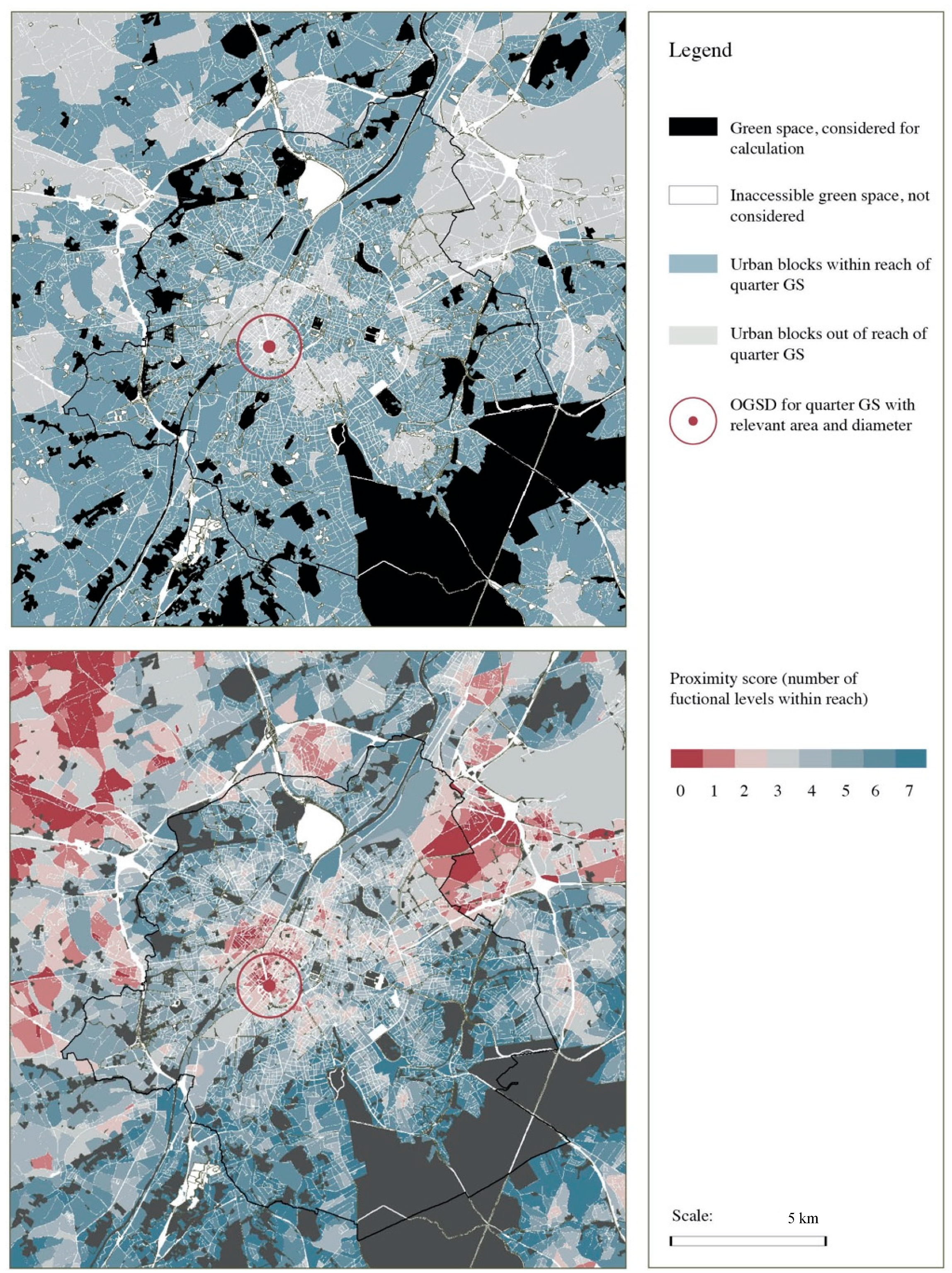
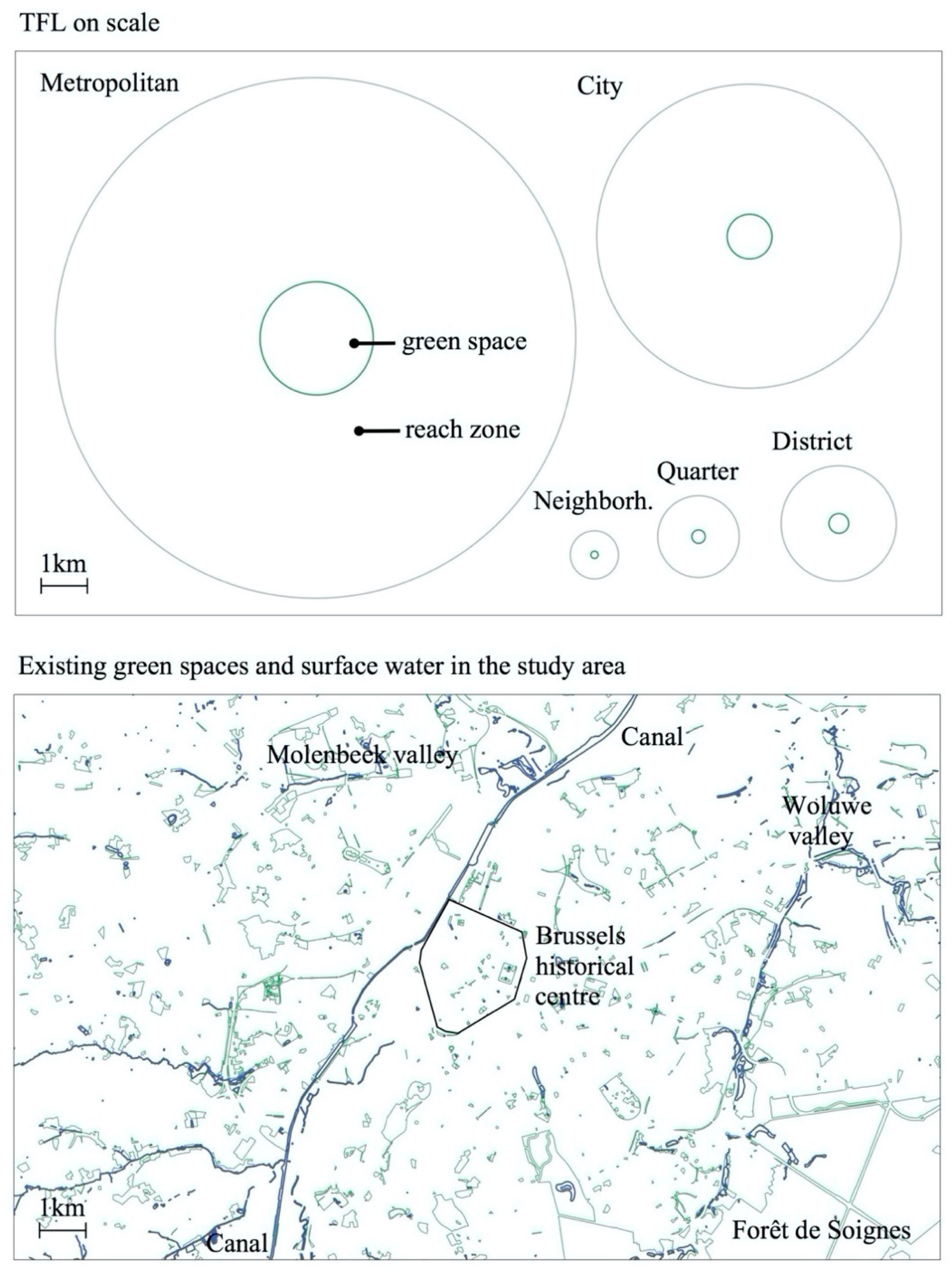
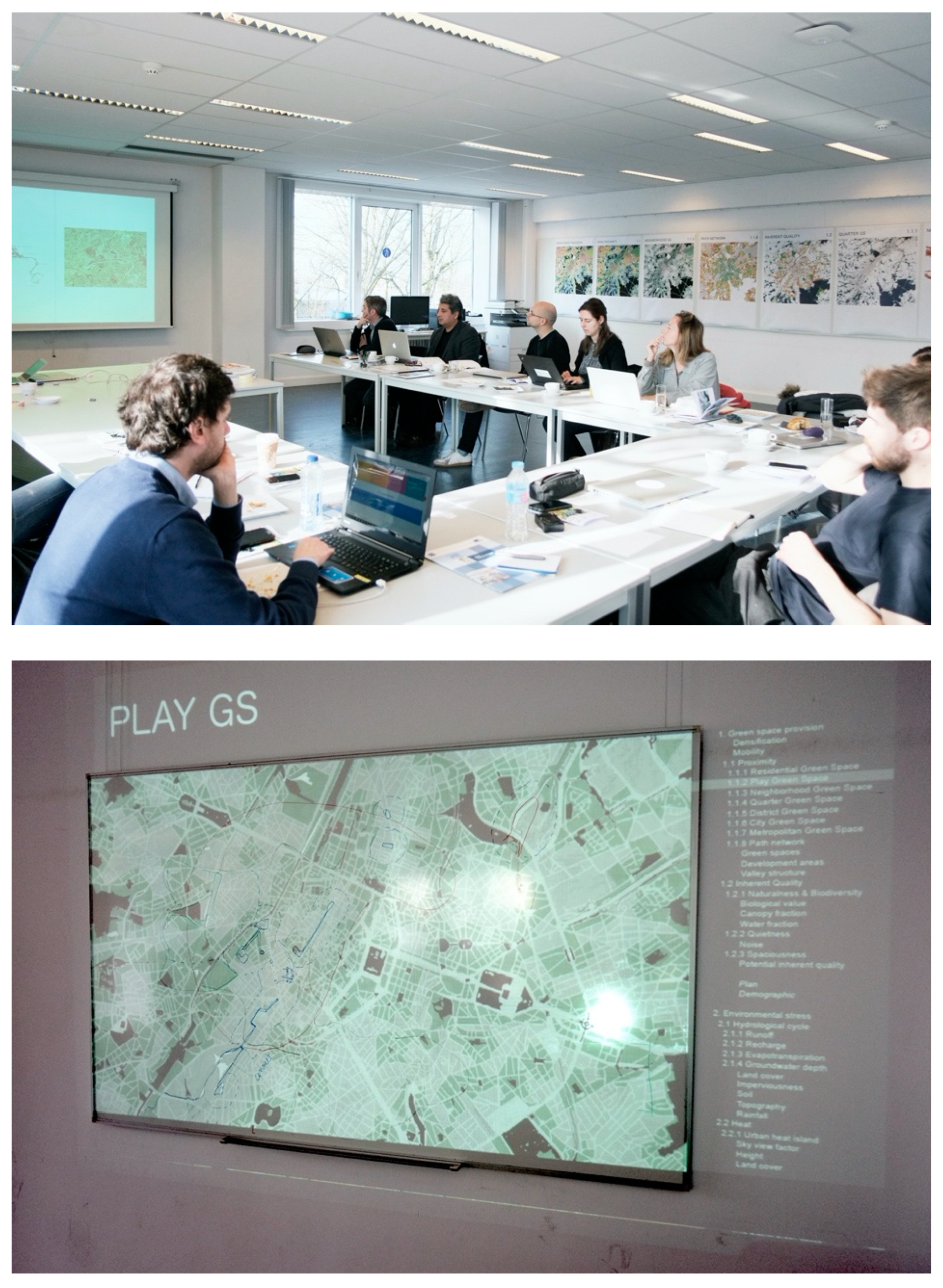

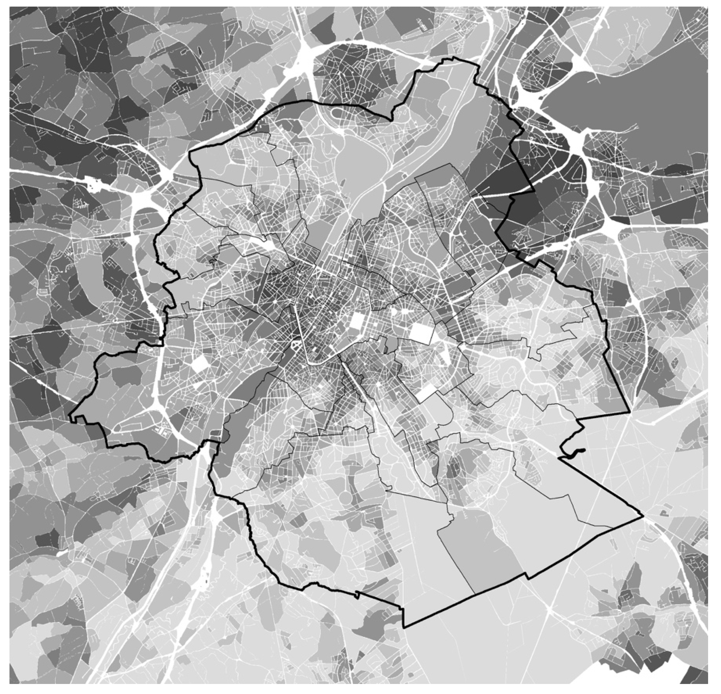

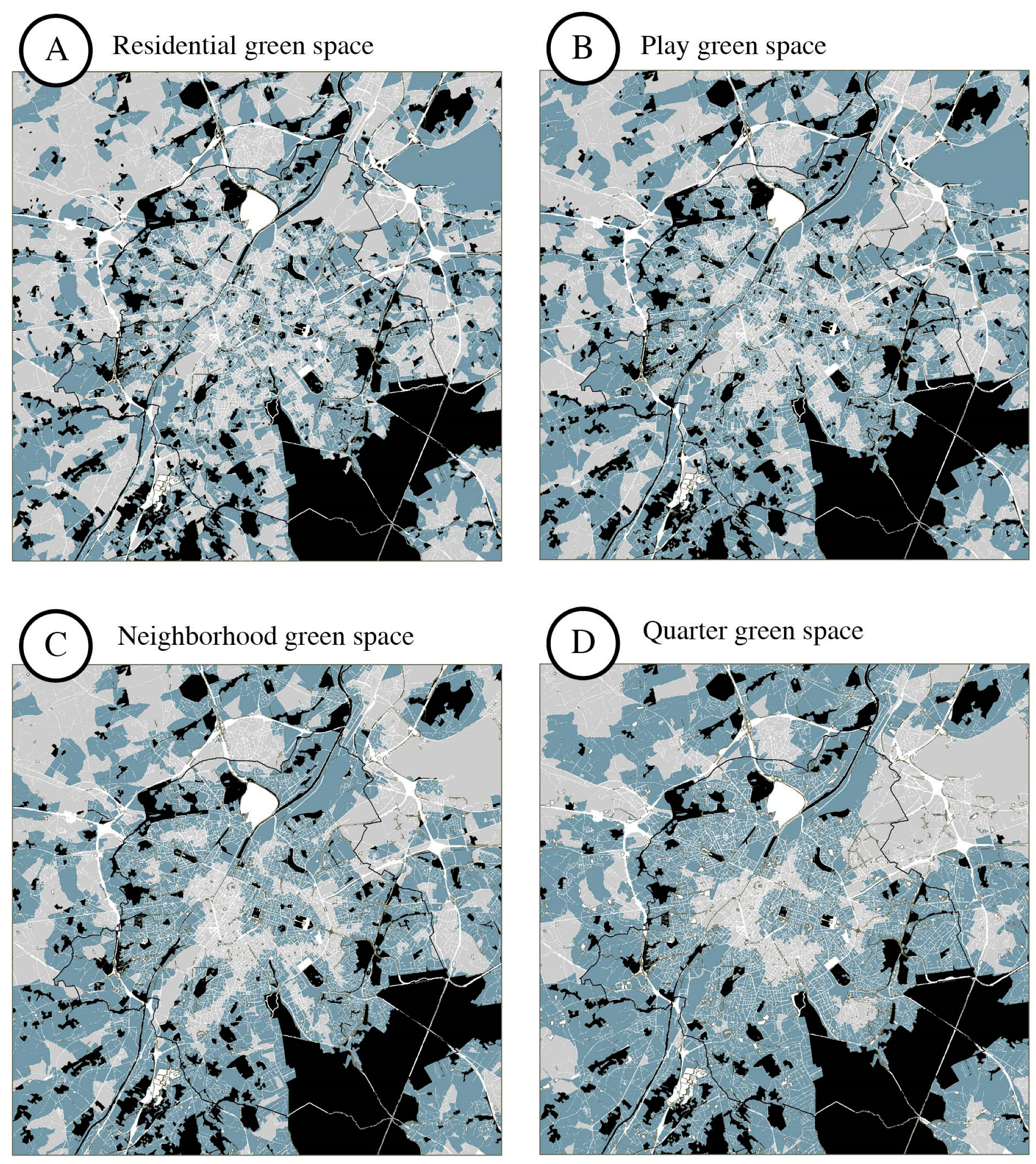
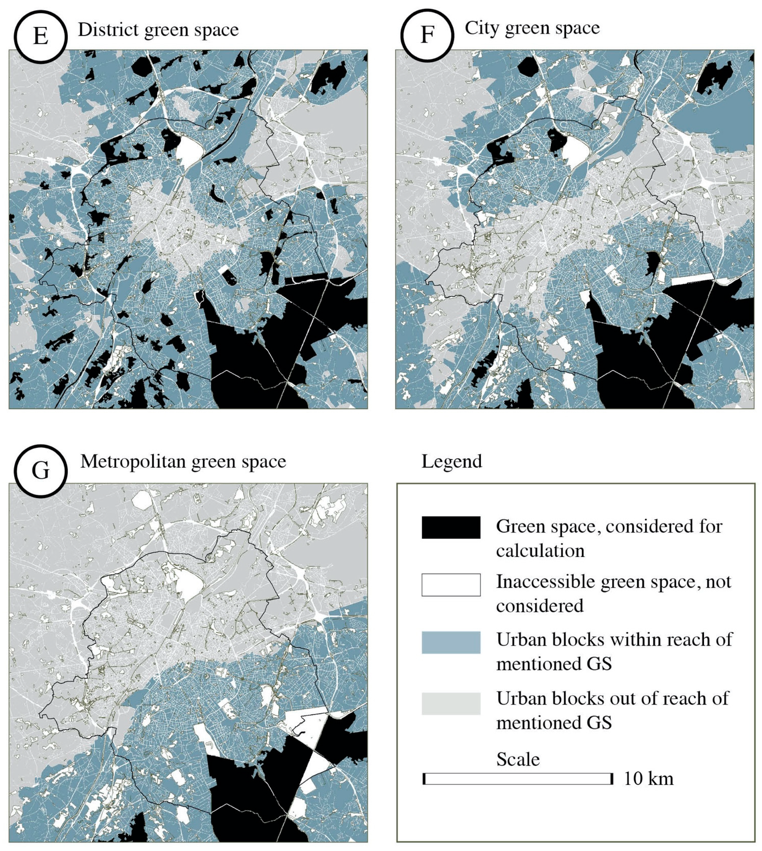
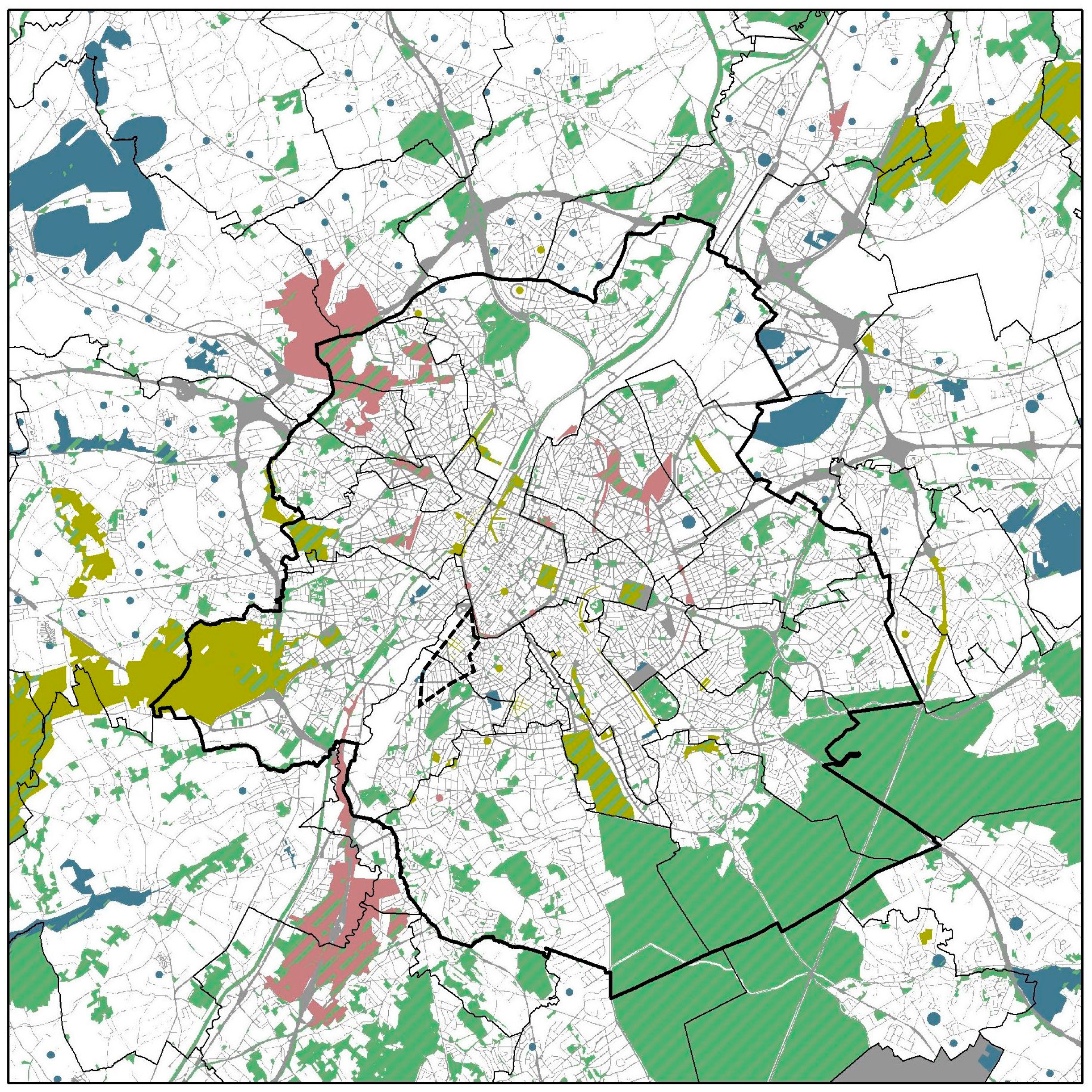
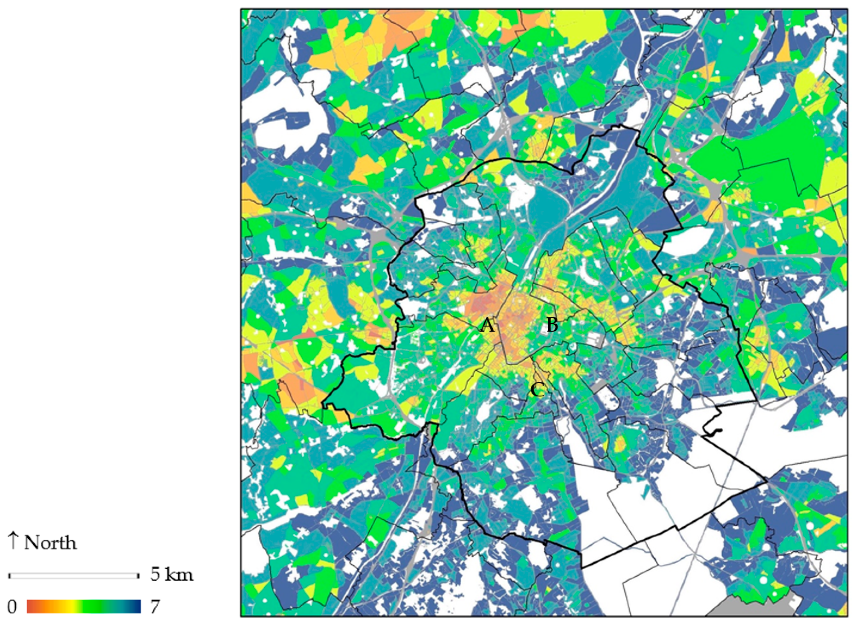

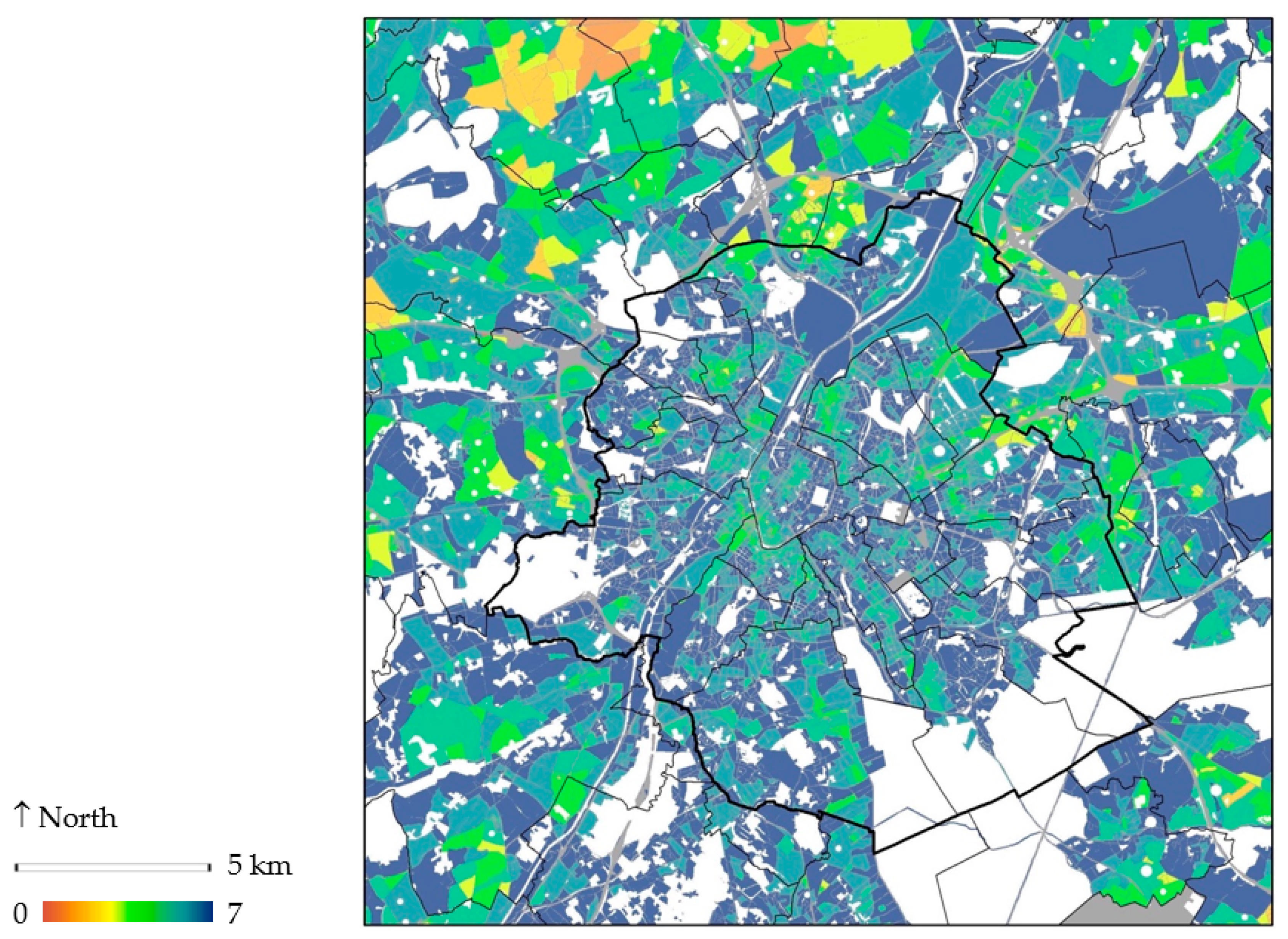
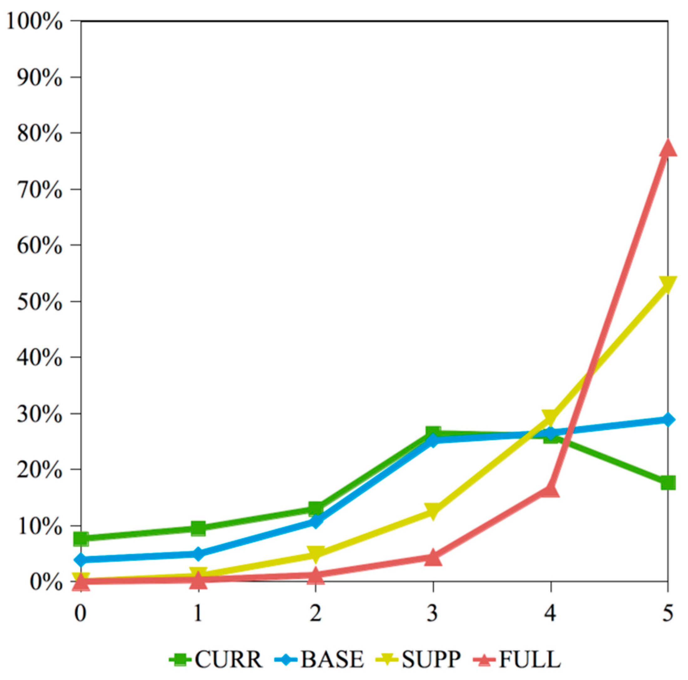
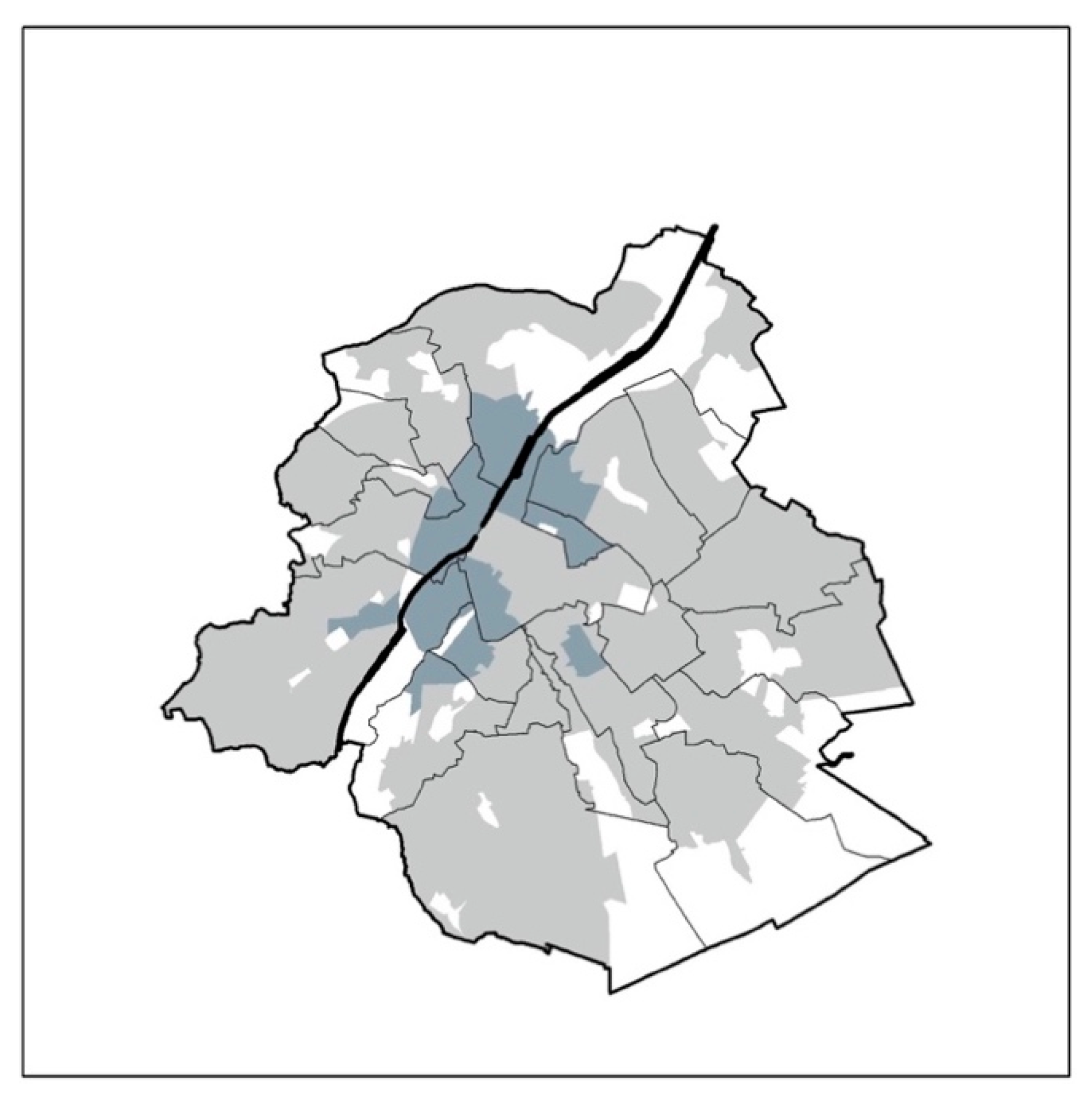
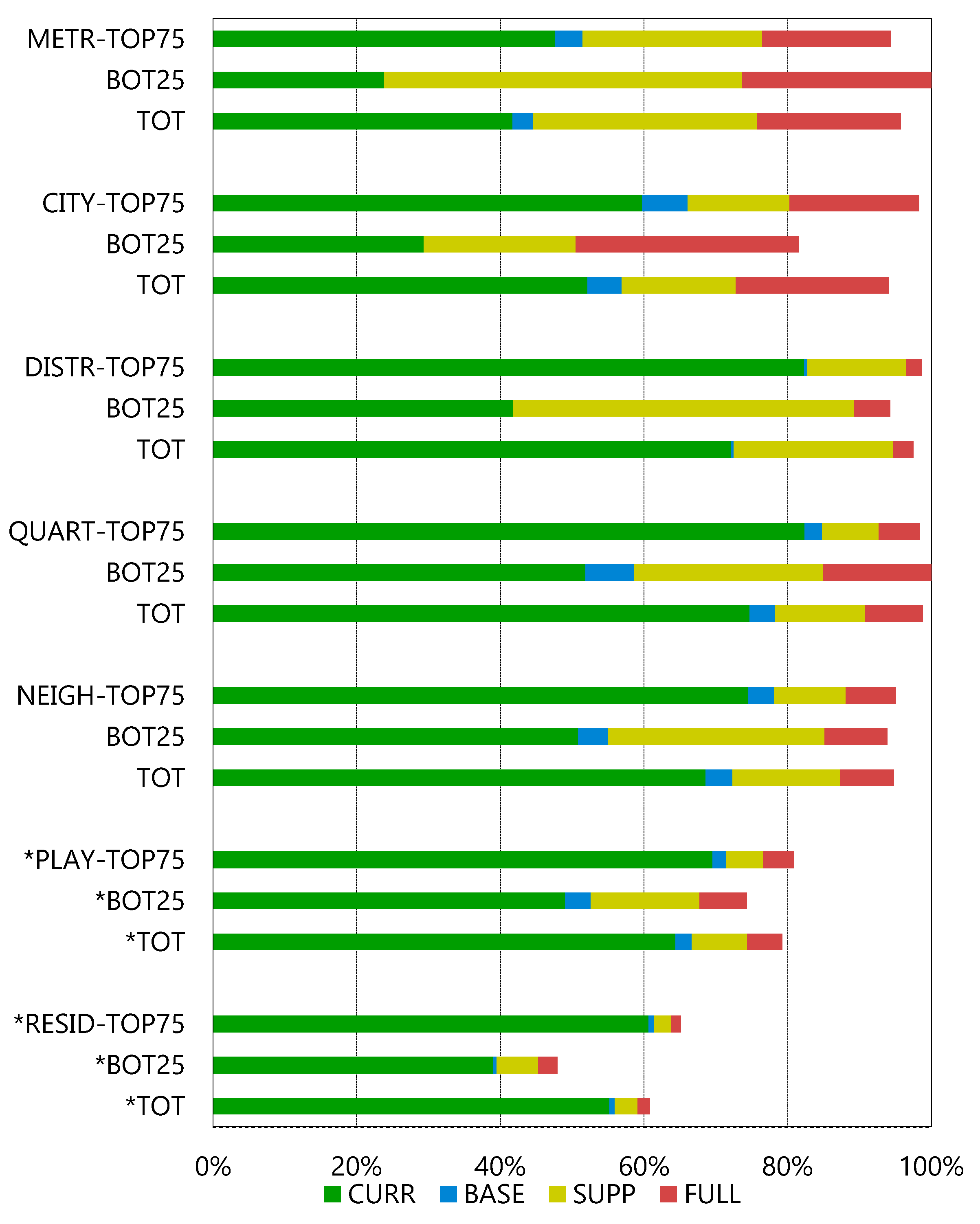
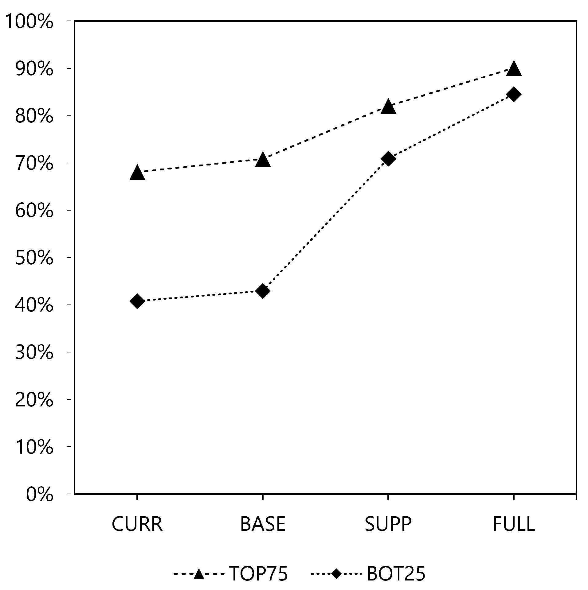

Publisher’s Note: MDPI stays neutral with regard to jurisdictional claims in published maps and institutional affiliations. |
© 2021 by the authors. Licensee MDPI, Basel, Switzerland. This article is an open access article distributed under the terms and conditions of the Creative Commons Attribution (CC BY) license (https://creativecommons.org/licenses/by/4.0/).