1. Introduction
With the rapid growth of the world economy and production scale, fossil fuel consumption and carbon dioxide emission from combustion increase day by day, and the phenomena of climate warming and environmental pollution are constantly highlighted. The resulting problems, such as “global warming” and “ecosystem deterioration”, are seriously threatening the living environment and development space of human beings [
1]. In recent years, the government of China has actively taken measures to reduce carbon emissions and advocate the development concept of “green GDP”. Transportation, especially cargo transportation, is one of the major energy consumers [
2]. According to the National Bureau of Statistics, the cargo turnover in China has increased from 4630.4 billion ton kilometers in 2001 to 19,929 billion ton kilometers in 2019 [
3]. How to deal with the relationship between the continuous growth of cargo transportation and carbon emission reduction is a severe challenge today.
As an important form of modern logistics, multimodal transportation can make use of the advantages of various modes to provide a more flexible and reliable choice for cargo transportation. Low-carbon multimodal transportation, which can realize the full use of energy by choosing transportation modes with low-carbon emissions, has become a hot issue in many countries. In 2020, the Ministry of Transportation in China put forward “the suggestions on promoting the modernization of transportation governance system and governance capacity”, establishing an advanced and efficient multimodal transportation application mechanism and improving the transportation energy conservation and emission reduction system [
4]. However, the data on cargo transportation in China in the past five years show that the proportion of road transportation is about 75% and presented an increasing trend year by year, while the proportion of railway and waterway transportation is about 10% and 14%, respectively. This proportion feature has failed to make full use of the advantages of the railway and waterway in transportation costs and carbon emission. To sum up, under the new economic situation of high-quality development, the low-carbon multimodal transportation route optimization research has important theoretical and practical significance, which can simultaneously meet the practical needs of the market, the economy and environmental protection, so as to realize energy conservation and emission reduction, promote the adjustment and upgrading of industrial structure and advance the low-carbon management of transportation industry.
Transportation is a complex system with many uncertain factors. Demand uncertainty is a common and difficult problem in the process of cargo trading based on the following two main reasons [
5]. On the one hand, it is because of inaccurate information communication among the trading companies, which lack real and effective information exchange. On the other hand, due to the advance of transportation planning, logistics service integration enterprises need to forecast the demand, but it is difficult for the forecast result to accurately reflect the fluctuation of a cargo demand similar to the bullwhip effect. In addition to the demand uncertainty, the randomness of transportation time should also be considered. Multimodal transportation path optimization is a typical non-polynomial problem, which is often affected by various emergencies or other unexpected events [
6], such as (1) vehicle maintenance; (2) traffic jam or anchoring in vehicle transportation; (3) emergency transportation; (4) vehicle performance; (5) differences in personnel capabilities; (5) road conditions, etc. [
7], which make it difficult for multimodal transportation to operate as planned. It has an impact on the entire operation and transportation time, and thus affects the multimodal transportation scheme.
The contribution of this paper is mainly reflected in two aspects. Firstly, the modeling contribution is the formulation of a hybrid robust-stochastic optimization model with double uncertainties of demand and time, including multiple scenarios of demand and uncertain collection of time. Secondly, the contribution of the research method is the catastrophe adaptive genetic algorithm based on Monte Carlo sampling, and the robust optimization problem with uncertain parameters is solved by Monte Carlo sampling. The results of a numerical example study can verify the effectiveness and efficiency of the model and the algorithm. In addition, we also observe the influence of uncertain parameters on decision-making and cost. Robust optimization with uncertain demand will increase the total cost, and the impact of time uncertainty on the total cost presents an irregular wave trend.
A brief review of the recent literature follows in
Section 2.
Section 3 defines the specific problems and related assumptions; in
Section 4, we establish the hybrid robust stochastic optimization model with dual uncertainty based on cost analysis;
Section 5 designs the model solution with adaptive genetic algorithm based on Monte Carlo sampling; in
Section 6, we verify the effectiveness of the model and algorithm by numerical examples and analyze the effect of uncertainty on decision-making; finally, some conclusions and future research problems are summarized in
Section 7.
2. Literature Review
The multimodal transportation path optimization problem has been relatively well-studied. Bontekoning et al. (2004) considered path optimization as a new and important field within the transportation research field [
8]. Janic (2007) built an optimization model of a multimodal transportation path with a time window to minimize the total cost [
9]. Liu et al. (2015) studied the multimodal transportation multi-objective optimization problem jointly solved by single-objective genetic algorithm and multi-objective genetic algorithm through model decomposition [
10]. Aiming at profit maximization, Ji et al. (2018) established an optimization model of a sea-rail intermodal container operation and designed a heuristic solving algorithm to obtain the optimal path and service pricing of railway transportation [
11]. However, the research of carbon emission in multimodal transportation has only recently been considered. The research on low-carbon multimodal transportation path optimization can be divided into the following two aspects.
Firstly, researchers try to prove the advantages of the multimodal transportation mode and path in low-carbon environmental protection. Liao et al. (2009) compared the carbon dioxide emission of single transportation and multi-modal transportation, and proved the applicability and superiority of the latter [
12]. Craig et al. (2013) calculated the carbon emissions in different modes of transportation and proved the advantages of multimodal transportation [
13]. Jiang et al. (2018) established a multi-objective decision-making model considering carbon emission, transportation cost and transportation time by analyzing the influencing factors of carbon emissions in container sea-land multimodal transportation, and concluded that the “railway-waterway-railway” multimodal transportation mode was the optimal scheme [
14]. The second aspect refers to the design and optimization of the multimodal transportation path considering low-carbon environmental factors. Bauer et al. (2010) designed the optimization model of a multimodal transportation path with carbon emission factors, and they believed that improving the transportation path could reduce carbon emissions and costs [
15]. Benjaafa et al. (2012) and Fahimnia et al. (2014) established a path planning model considering the transportation costs and carbon emissions simultaneously. The former pointed out that the choice of transportation mode, distribution frequency and coordination relationship between enterprises had a great impact on carbon emissions, while the latter solved the model by using an improved cross entropy algorithm [
16,
17]. Bouchery et al. (2015) established a two-target dynamic multimodal transportation model including transportation cost and carbon emissions, and determined a specific low-carbon transportation scheme [
18]. Cui et al. (2014) and Duan et al. (2015) designed the low-carbon synergies evaluation equation and model of various transportation modes. On this basis, an “axle-spoke” container shipping network optimization model with carbon emissions was constructed [
19,
20]. Wang et al. (2014) proposed a new irregular prism network model to realize the intelligent optimization of multimodal transportation paths and modes [
21]. Cheng (2019) studied the impact of carbon emission policies, including mandatory carbon emission, carbon tax, carbon trading and carbon compensation on carbon emission reduction and the cost of multimodal transportation [
22].
Uncertainty has become an important feature of today’s society. It can be seen that stochastic programming [
23], fuzzy programming [
24], robust optimization [
25] and fuzzy-based hybrid methods [
26,
27,
28] are the effective ways to solve the uncertainty problems in multimodal transportation. The uncertainty in low carbon multimodal transportation can be divided into the uncertainty related to demand, transportation time and carbon emissions. For the demand uncertainty in multimodal transportation, Ramezani (2013) proposed a random multi-objective model of forward/reverse logistics network designing under an uncertain environment [
29]; Demirel et al., (2014) solved the problem of multimodal transportation route selection in the case of fuzzy demand by introducing triangular fuzzy numbers [
30]. Li et al., (2018) established an opportunistic constrained multi-objective robust-fuzzy programming model considering the fuzziness of multi-stage closed-loop supply chain network parameters [
31]; Zhang et al., (2020) researched the multimodal transportation path optimization problem under demand uncertainty using robust optimization [
24]. In terms of uncertain transportation time, Adil et al., (2019) optimized the overall transportation cost and customer satisfaction by simultaneously considering the random cargo demand and fuzzy transportation time [
32]; Jiang et al., (2020) constructed the optimization model of a container multimodal transportation path, taking the transportation time and transfer time as random numbers [
33]. For the carbon emissions uncertainty, Gao and Ryan (2014) considered a robust formulation of a multi-period capacitated CLSC network design problem while considering two regulations for carbon emissions [
34]; Yu-Chung et al., (2018) solved the low carbon network design problem using nonlinear optimization technology, which took the uncertainty related to a carbon tax and carbon emissions into consideration [
35]. In the study of Ali et al., (2018), the randomness of the carbon tax was considered, and an optimization model of low-carbon multimodal transportation route was established [
36].
Based on the above analysis, studies on low-carbon multimodal transportation have been relatively mature, but most of them focus on a deterministic environment, and there are few studies on uncertain scenarios, especially dual or multiple uncertain scenarios. Considering the characteristics and requirements of China’s carbon emission policies, we take carbon emissions as determining factors, and our study combines two types of uncertainties mentioned above, namely, uncertain demand and random time, including transportation and transshipment. To model demand uncertainty, we formulate a robust optimization, which was first proposed by Soyster (1972) [
37]. Meanwhile, the stochastic transportation time is regarded as a set of random numbers following a normal distribution. Therefore, in our hybrid robust-stochastic low-carbon multimodal transportation path optimization problem, we integrated robust optimization and stochastic programming to deal with uncertainty in the demand and transportation time. In addition, we design the catastrophe adaptive genetic algorithm based on Monte Carlo sampling, verify the validity of the model and algorithm through an example, and analyze the uncertain parameters’ influence on the transportation scheme and cost. We show that the changes in demand and time will have an impact on the path and mode of transportation. This paper can enrich the modeling and solving methods of robust optimization with uncertain parameters, and, further, provide low-carbon transportation decision-making references for the multimodal transportation operators.
3. Problem Description and Hypothesis
This study envisages a situation where a batch of cargo from starting point O to destination D is transported by a logistics service provider, and there are three transportation modes, including road, water and rail, to choose from. During this period, the cargo will pass through several transportation nodes using one of the alternative transportation modes, and meanwhile each mode has its own transportation costs, time, carbon emissions and costs. On the one hand, due to the advance of the multimodal transportation plan and the volatility of demand, the logistics service provide the need to determine the cargo transportation plan under uncertain demand. On the other hand, the transportation process can be inevitably affected by various emergencies, and the total time is random and difficult to determine
The aim of this essay is to explore the transportation path and mode that can not only meet the requirements of transportation cost, time and carbon emission, but also achieve the stability of the robust optimization model in the double uncertainty of demand and time.
The research hypothesis is as follows:
(1) The same batch of cargo is indivisible in the process of transportation, that is, it can only be transported as a whole unit in the process of transportation, and cannot be divided into two or more parts;
(2) Each transportation node has sufficient transshipment capacity, and the waiting time and its cost during transshipment can be ignored;
(3) Transshipment can only occur at the transportation node, and at this node, the transportation mode of each batch of cargo can be changed at most once;
(4) All nodes can meet the transshipment requirements of each transportation mode, and there is no difference in transshipment time and cost;
The transportation capacity of different modes can always meet the requirements of the cargo volume.
The following parameters and decision variables in
Table 1 will be used in the formulation of the low-carbon multimodal transportation path optimization problem under double uncertainty.
4. Hybrid Robust Stochastic Optimization (HRSO) Model
In the dual uncertain low-carbon multimodal transportation path optimization problem, the uncertainty of cargo demand and total time should be considered at the same time. We add the time cost related to the random transportation and transshipment time to the traditional low-carbon path optimization model. Meanwhile, different demand situations and their adaptability to model constraints and targets are also analyzed. The model construction idea is as follows: the first step is to determine the cost composition and its calculation method in low-carbon multimodal transportation; secondly, the total transportation time should be expressed as a random number in the uncertain demand situations; at last, a hybrid robust stochastic optimization (HRSO) model of low-carbon multimodal transportation path can be established.
4.1. Total Transportation Cost
The total transportation cost consists in the direct transportation cost between nodes and the transshipment cost on each node, which can be expressed in the form of Equations (1) and (2), respectively. The former is the product of the cargo volume, the transportation distance and the unit transportation price, while the latter is the product of the cargo volume and the unit transshipment cost corresponding to the transportation mode.
4.2. Total Time Cost
The total time consists of the transportation time between nodes and the transshipment time on each node, as shown in Equation (3).
The first half of Equation (3) is transportation time, which is expressed by the ratio of distance to speed, i.e., , while the second half is transshipment time, which is calculated by the product of cargo volume and unit transshipment cost corresponding to the transportation mode, i.e., .
Based on this, the time cost consists of two parts: the warehousing cost for early arrival and the penalty cost for late arrival. If the cargo arrives in advance, before the lower limit of the time window, a certain warehousing cost shall be paid; on the contrary, if the cargo arrives late, after the upper bound of the time window, there will be a corresponding penalty cost.
The time cost is linearly related to the transportation time, which can be expressed in the form of Equation (4).
4.3. Total Carbon Emission Cost
In recent years, various countries have adopted different emission reduction measures, such as carbon emission trading, cap-and-trade, technical standards and a carbon tax. Among them, carbon trading is a concept in the Kyoto Protocol, which takes carbon emission rights as commodities and forms a new strategy to solve emission reduction problems through market trading, which has been widely adopted by the United Nations, the European Union and many other countries or international organizations. The rationale for carbon trading is the carbon quota, which can be bought or sold. The companies can either purchase the additional quota or sell the extra quota, and they can change the total cost through the carbon trading cost or benefit. China officially launched its carbon trading market in December 2012, and eight provinces and cities, including Beijing, Fujian, Guangdong, Hubei, Shanghai, Shenzhen, Tianjin and Chongqing, are taken as the pilots. In this study, carbon emission costs or benefits are calculated based on the carbon trading policy. In other words, the emission cost will increase when the carbon emission exceeds the emission quota Q; otherwise, the emission cost will decrease by selling the unused carbon quota. See Formula (5) for the total carbon emissions generated in multimodal transportation.
Among them, the carbon emissions in transportation are calculated by the production of unit carbon emissions, cargo volume and transportation distance, which is . The carbon emissions in transshipment are expressed as the carbon emission coefficient and cargo volume, i.e., .
Therefore, based on the characteristics of carbon trading policy, the carbon emission cost can be expressed in the form of Formula (6).
4.4. HRSO Model with Dual Uncertainty
As an effective method to study uncertain optimization, robust optimization is widely used in production scheduling, transportation planning and supply chain management. In order to analyze the dual uncertainty of cargo demand and total transportation time, the concept of robust optimization is applied to the optimization model of the multimodal transport path:
The uncertainty of the cargo demand is represented by the scenario approach in robust optimization. Suppose that there are S demand scenarios, the uncertain demand in each scenario is and their occurrence probability is .
For the time uncertainty, the transportation time and transshipment time are set as random numbers subject to normal distribution, namely
,
, where
and
represent the mean and variance of transportation time, and
and
represent the mean and variance of transshipment time separately. According to the Lyapunov’s central limit theorem, the sum of multiple independent random variables follows a normal distribution; then:
Therefore, the total transportation time obeys the normal distribution of mean value and variance , i.e., .
In summary, the optimization problem of the low-carbon multimodal transportation path with dual uncertainty of demand and time can be abstracted into a hybrid robust stochastic optimization model (HRSO) combining a scenario method and stochastic programming. The HRSO model is shown below.
Formula (9) is a prototype of the objective function based on scenario robust optimization under the dual uncertainty of demand and time, which is composed of transportation cost, time cost and carbon emission cost under scenario . Formula (10) constrains the range of total time , which is subject to a normal distribution of mean and variance . Formula (11) is a constraint related to demand uncertainty, which limits the proximity of each feasible solution to the optimal value of scenario . In this formula, is the allowable objective function value of scenario , is the optimal objective function of deterministic problems of scenario , and, always, . In addition, is called the maximum regret value, which indicates the maximum deviation between the allowable objective function value and the optimal objective function value; specifically, it was a deterministic demand when . Equation (12) indicates that the sum of the occurrence probability of each scenario is 1. In Equation (13), only one transportation mode can be used at most between nodes and . Equation (14) is the constraint that transshipment at one node can only occur at most once. Equation (15) requires that if the cargo is transshipped at one node, its transportation mode should be consistent with the mode before and after the node. Equation (16) defines the decision variable as a 0–1 variable.
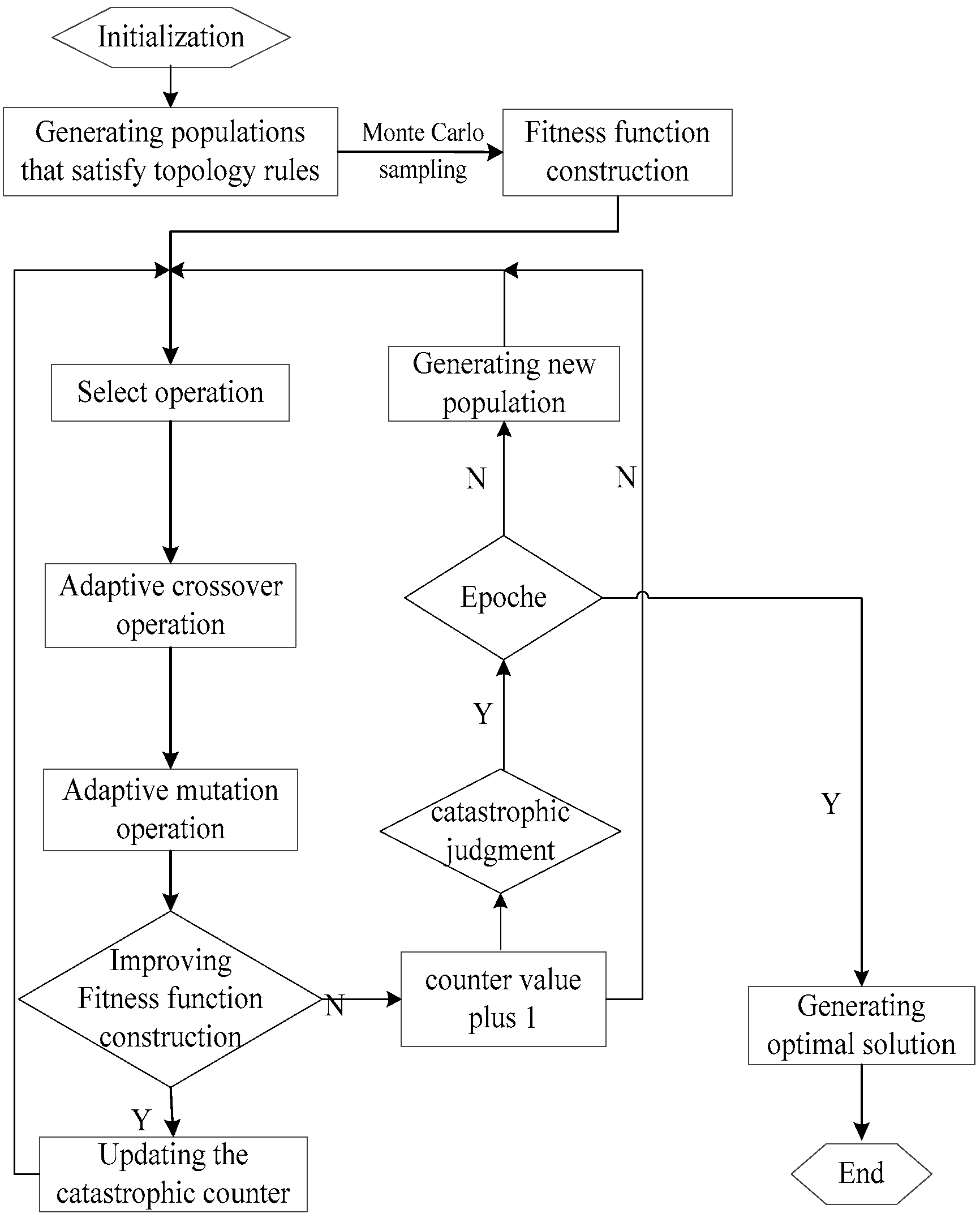
5. Catastrophic Adaptive Genetic Algorithm (CA-GA) Based on Monte Carlo Sampling
The multimodal transportation path optimization problem under dual uncertainty needs to determine the transportation path and mode under robust demand and random time. The model involves many intermediate variables, and it is a typical NP-hard problem [
38]. In view of the proposed HRSO model with uncertain parameters, the traditional genetic algorithm is partially improved, and the catastrophic adaptive genetic algorithm (CA-GA) based on Monte Carlo is designed to prevent premature convergence and improve the global search performance. These specific improvements include: (1) adding topological sorting rules when generating the initial population based on the characteristics of the research problem; (2) constructing a fitness function based on the Monte Carlo sampling method; (3) designing adaptive crossover and mutation operation; (4) adding catastrophic operator to the genetic operation. The algorithm ideas and steps are as follows.
5.1. Chromosome Coding
The problem of the multimodal transportation path optimization is a combinatorial optimization problem; therefore, a two-layer coding structure is adopted. The first layer is the coding of the transportation path, and the second layer is the coding of the transportation mode. All of these layers are coded by real numbers, as shown in Equation (17). Each coding corresponds to a transportation scheme, representing the transportation path and mode from the starting point to the end.
In Formula (17), M is the number of transportation nodes, and N is the number of transportation modes.
5.2. Population Initialization Based on Topological Sorting
The nodes in the multimodal transportation are arranged in a certain order. In order to ensure the feasibility of the solutions, the initial population is generated based on topological sorting rules to suppress the generation of illegal schemes. The multimodal transportation topology order is obtained by the following methods.
(1) Design the transportation paths in the transportation diagram into a directed acyclic graph;
(2) Place the directed acyclic graph in the topological sorting sequence to obtain the topological sorting of the network graph.
In addition, it is useful and necessary to deal with the relationship between population diversity and algorithm efficiency when determining the initial population size. In practice, it is mainly determined according to the experience of decision makers or the problem’s characteristics.
5.3. Fitness Function Based on Monte Carlo Sampling
The fitness function construction of the genetic algorithm is an important link that directly affects the convergence rate and the optimal solution [
39,
40]. For the HRSO model with uncertain parameters, the pseudo-random numbers in Monte Carlo sampling are used in this study to construct the fitness function.
The uncertain parameter is obtained by the random sampling from the probability density distribution function U. Suppose that the mean value and variance of the corresponding objective function of decision variable under different are, respectively, and .
Then, according to the characteristics of this optimization problem, the smaller
and
can reflect the pursuit of the minimization of the objective function and its fluctuation. Therefore, the fitness function of the optimization problem can be expressed as Formula (18).
5.4. Genetic Operation
5.4.1. Select Operation
The select operation uses the common roulette selection method, that is, the probability
of an individual to be selected is determined according to the fitness of chromosomes, as shown in Formula (12), where I is the population size and
is the fitness of an individual.
5.4.2. Adaptive Crossover and Mutation Operation
The adaptive adjustment of crossover and mutation is one of the main methods of the adaptive genetic algorithm. The crossover probability and mutation probability are dynamically adjusted according to the fitness value, which can improve the global and local convergence performance of the genetic algorithm. The following formulas are used to represent the dynamic crossover probability
and the mutation probability
.
In Formulas (20) and (21), and are the initial crossover probability and the mutation probability, respectively. is the average fitness of the population, and is the larger fitness among the crossover or
mutation individuals. are the constants between 0 and 1.
5.5. Catastrophic Operator
In order to reduce the “precocious” phenomenon in the algorithm, a catastrophic operator is added to the traditional genetic algorithm. In other words, the catastrophe will be initiated when there is still no new optimal solution generated in the optimization search process for multiple generations, and the local search will be actively removed from the algorithm. The global search capability of the algorithm can be enhanced through this catastrophic operator. The catastrophe counter is used to judge the conditions of catastrophe in this research, and the specific catastrophe mode is as follows.
Set a catastrophe counter whose initial value is 0, and the catastrophe counter value plus 1 for each generation of new individuals. This means that the optimization results did not change many times and the local search has been fully adequate if the catastrophe counter value exceeds a specific value . In this situation, the catastrophe which includes re-selecting the best individuals and performing genetic operation can be initiated. In detail, the diverse individual tournament selection mechanism is used to select the reserve individuals, that is, % of the individuals in the population would be randomly selected for comparison, and the chromosome with the best performance among these individuals will be selected for the next stage of genetic operation. On the contrary, if a new optimal solution appears in the counting process, the catastrophe counter will return to zero.
In conclusion, the process of CA-GA based on Monte Carlo sampling to determine the optimization scheme of the multimodal transportation path under dual uncertainty of demand and time is shown in
Figure 1.
6. Numerical Example
6.1. Basic Scenario and Data
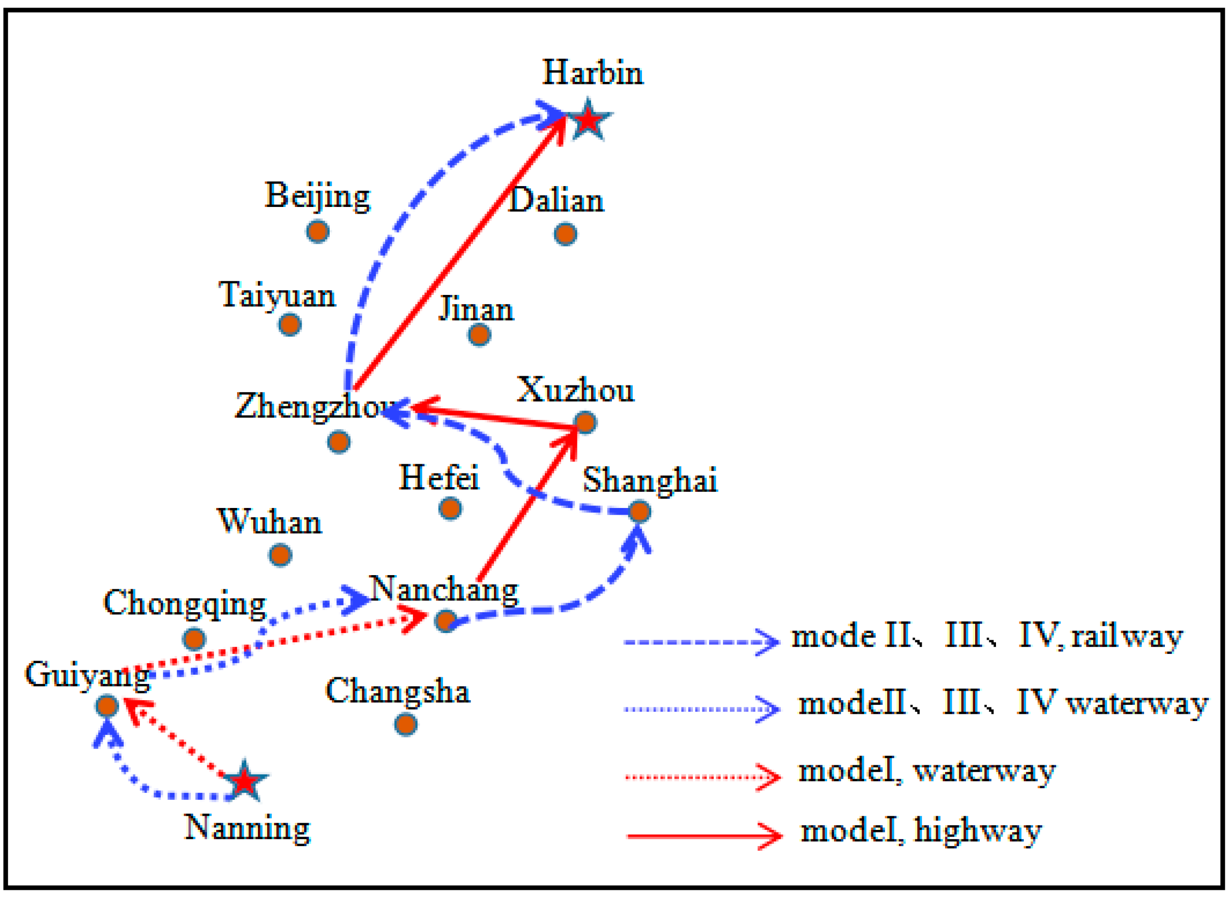
The numerical scenario considers that an enterprise providing multimodal transportation services will transport a batch of cargo from Nanning, the starting point, to Harbin, the destination point, by a joint transportation network containing 15 nodes. The node numbers O, 1, 2…, D are, successively, Nanning, Guiyang, Chongqing, Nanchang, Changsha, Wuhan, Hefei, Shanghai, Xuzhou, Jinan, Zhengzhou, Taiyuan, Beijing, Dalian and Harbin. The specific network is shown in
Figure 2.
The transportation distance data of different modes between cities are obtained through Amap, the train ticket network (
https://www.12306.cn/, accessed on 27 June 2020), the ship ticket network and the related literature. The specific distance data are shown in
Table 2, where (a,b,c) represents the transportation distance of highways, railways and waterways, respectively, and “—” means that there is no transportation mode or route between two adjacent nodes.
According to the objective reality, this research supposes that the cargo must arrive within the time period (55, 65) h. The unit storage fee for early arrival is 15 yuan/hour∙ton, and the unit penalty cost for late arrival is 30 yuan/hour∙ton. The emission quota for the transportation mission is 4 ton, and the carbon trading price is set to 30 yuan/ton based on the statistical data of the “Carbon K Line”, developed by the China Carbon Information Technology Research Institute
The relevant parameters of transportation and transshipment by various modes of transportation are obtained based on the price of the railway freight service and the settings in the existing literature [
38]—see
Table 3 and
Table 4. Among them, the transportation time follows a normal distribution, and the transportation speeds of different modes are used to calculate the mean value of the time. In
Table 2, (a,b,c) represents the benchmark transportation price between the nodes whose distance is in the range of “mileage ≤ 500 km”, “500 km < mileage ≤ 1000 km” and “1000 km < mileage”, respectively.
Due to the advance in transportation planning, the cargo demand is difficult to predict. Considering the daily data of the actual cargo volume, as well as the attention to high and low volume situations, we set the cargo volume and its corresponding probability under different scenarios of high, middle and low as 150t (0.36), 85t (0.5) and 40t (0.14), respectively.
6.2. Algorithm Validity
The proposed CA-GA based on Monte Carlo sampling is adopted by Matlab2016 programming in order to verify its performance. The parameters of the algorithm are set as follows: the population size is 80, the number of iterations is 200, the initial crossover probability is 0.8, the initial mutation probability is 0.3, the critical value of the catastrophic counter is 50 and the catastrophic proportion is 10%. In addition, the maximum regret value α in robust optimization is set to 0.2.
Taking the model of deterministic demand and time as an example, the traditional GA and the CA-GA in this paper are respectively used to conduct 10 optimization tests. The optimization results and average running time are shown in
Table 5.
In
Table 5, the running time of CA-GA is slightly higher than that of the traditional GA. It is affected by the changing crossover and mutation probability, the number of catastrophes and the number of iterations between two catastrophes in CA-GA, which makes the algorithm operation more complicated and the termination conditions more difficult to reach accordingly.
As regards the optimization results, the target value of CA-GA in
Table 4 is obviously better than that of the traditional GA. In the 10 calculations, GA-CA obtains the optimal value of 112,054.39 four times, while the traditional GA achieved the optimal value only once. At the same time, from the average target value and the worst target value, CA-GA is obviously superior to GA. Compared with the traditional GA, CA-GA can obtain more excellent individuals and schemes due to the addition of catastrophic operators and adaptive crossover and mutation operations.
6.3. Results Analysis
6.3.1. Results Comparison
For a more comprehensive analysis of the transportation scheme and cost, four contexts are designed, including deterministic demand and time (demand is the mean value of three scenarios, time variance is 0, mode I), deterministic time and uncertain demand (maximum regret value α = 0.2, mode II), deterministic demand and uncertain time (time variance as Formula (8), mode III), and uncertain demand and time (mode IV). The transportation scheme (see
Figure 3) and cost (see
Table 5) of each mode are calculated by the proposed CA-GA.
According to
Table 6, the total cost of the four modes is sorted as “mode IV > mode II > mode III > mode I”, and the specific comparative analyses are as follows.
(1) Mode I is the basic mode, whose demand and time are both deterministic. In this mode, the transportation path is “O-1-3-8-10-D”, and the transportation modes are, respectively, waterway, waterway, highway, highway and highway. There is only one transshipment, and the final total cost is 112,054.39 yuan.
(2) Mode II, III and IV are all uncertain modes, which meanwhile have the same transportation path and modes. In the aspect of cost, mode II increases by 12,859.72 yuan compared with mode I, which indicates that the uncertainty of demand has a significant impact on the cost of multimodal transportation; mode III increases by 6546.17 yuan compared with mode I, which is mainly caused by the change of time; mode IV has the largest total cost, which increased, respectively, by 0.4% and 5.8% compared with modes II and III. This is mainly caused by the different influence mechanism of uncertain demand and stochastic time, i.e., the uncertain demand affects cost by the maximum regret value constraints in robust optimization, while the stochastic time changes the cost through the random number and its distribution.
6.3.2. Impact of Uncertainty on Cost and Decision Making
(1) The impact of demand uncertainty on cost and decision-making
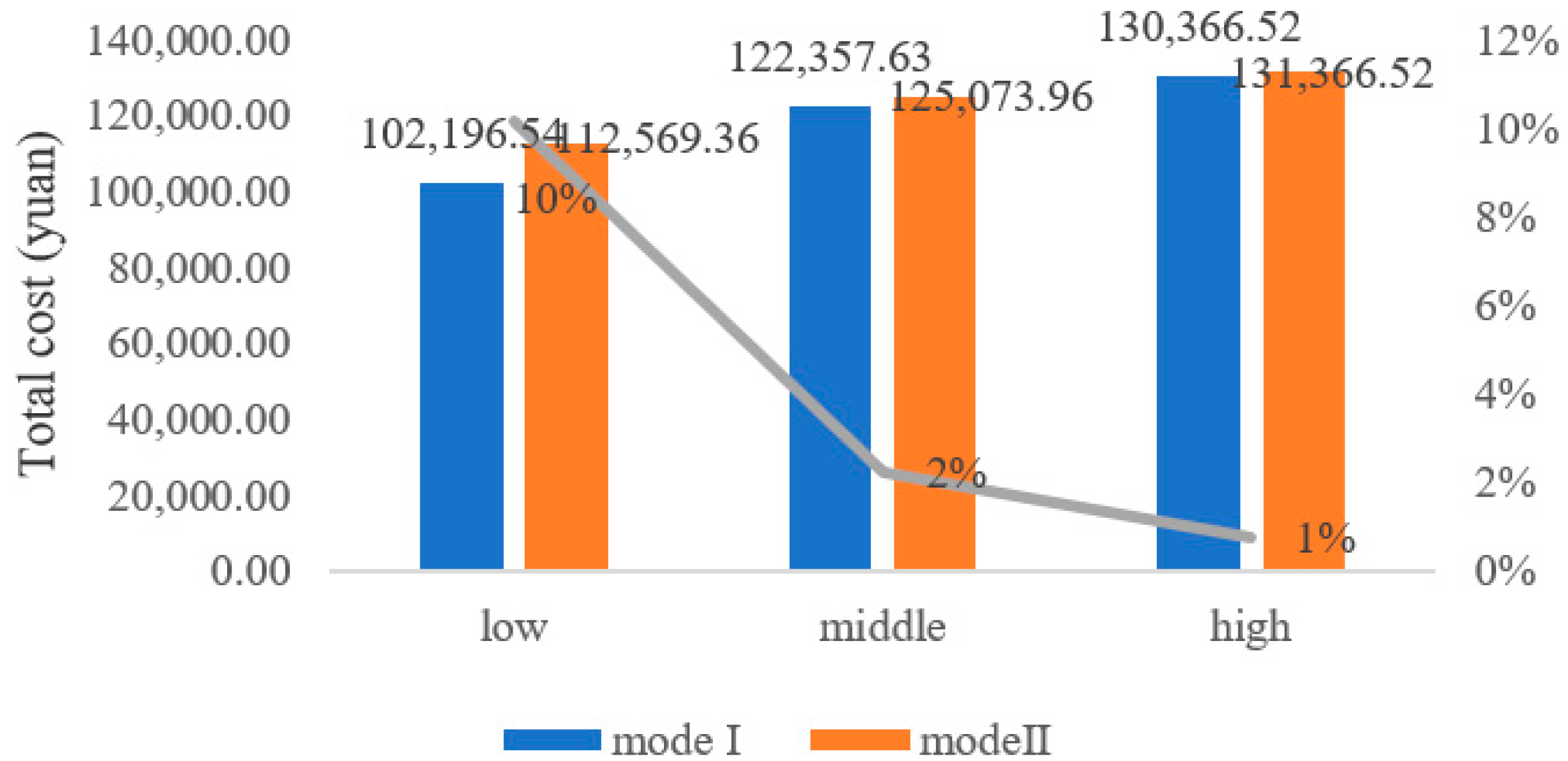
The total cost under different scenarios, including low, medium and high, can be obtained by taking the transportation path and mode of mode II into different cargo volumes.
Figure 4 shows the total cost comparison results between Mode I and Mode II under three demand scenarios. Among them, the total costs of the three scenarios in mode II are not all lower than the total costs of mode I, which indicates that robust optimization, as a method focusing on the stability of the target, has a certain conservatism in solving uncertain problems.
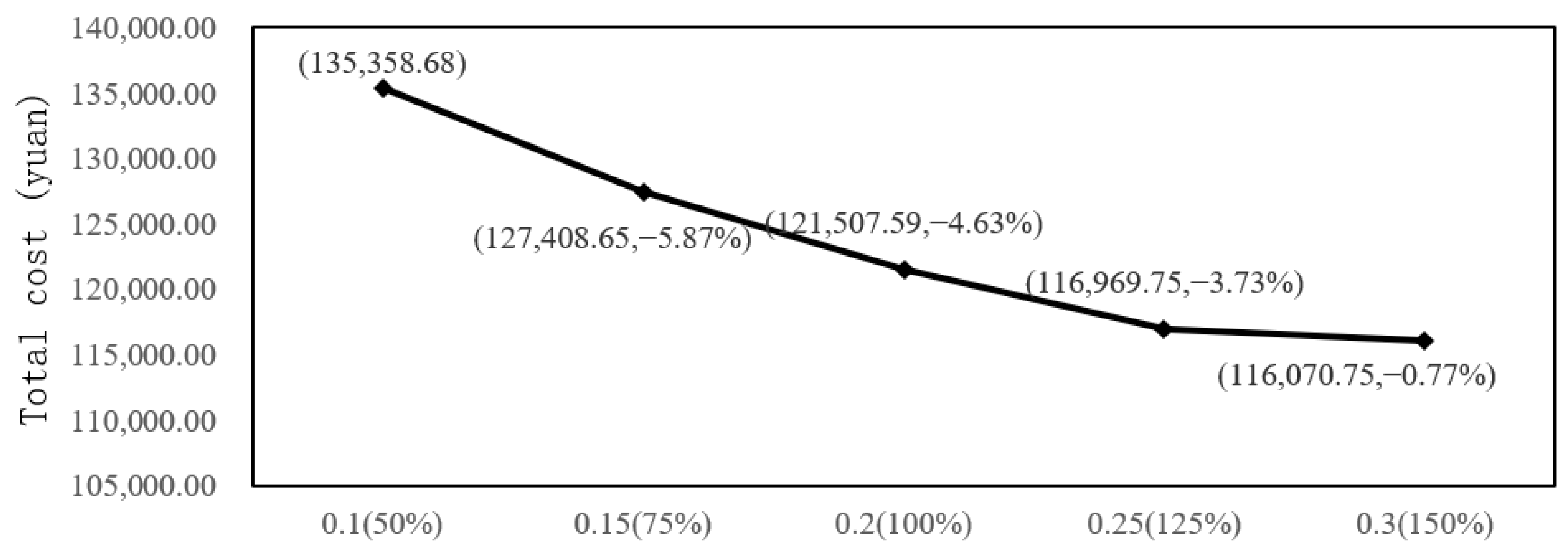
Further, the parametric sensitivity analysis is performed for the maximum regret value under mode IV to explore the influence of demand uncertainty on cost and decision making under dual uncertainty. The results are shown in
Figure 3. Among them, the total cost decreases with the increase of the maximum regret value, which further verifies the fact that robust optimization pays more attention to stability. The curve in
Figure 3 is characterized as “steep edge and flat ground”, when
, the total cost decreases quickly and, accordingly, when
, the reduction in the total cost is relatively smooth. Therefore, the strong robustness of multimodal transportation does not necessarily mean that the total cost will increase significantly. Decision-makers may be able to improve the operation efficiency of multimodal transportation by weighing the relationship between the maximum regret value and the cost.
(2) The impact of time randomness on cost and decision
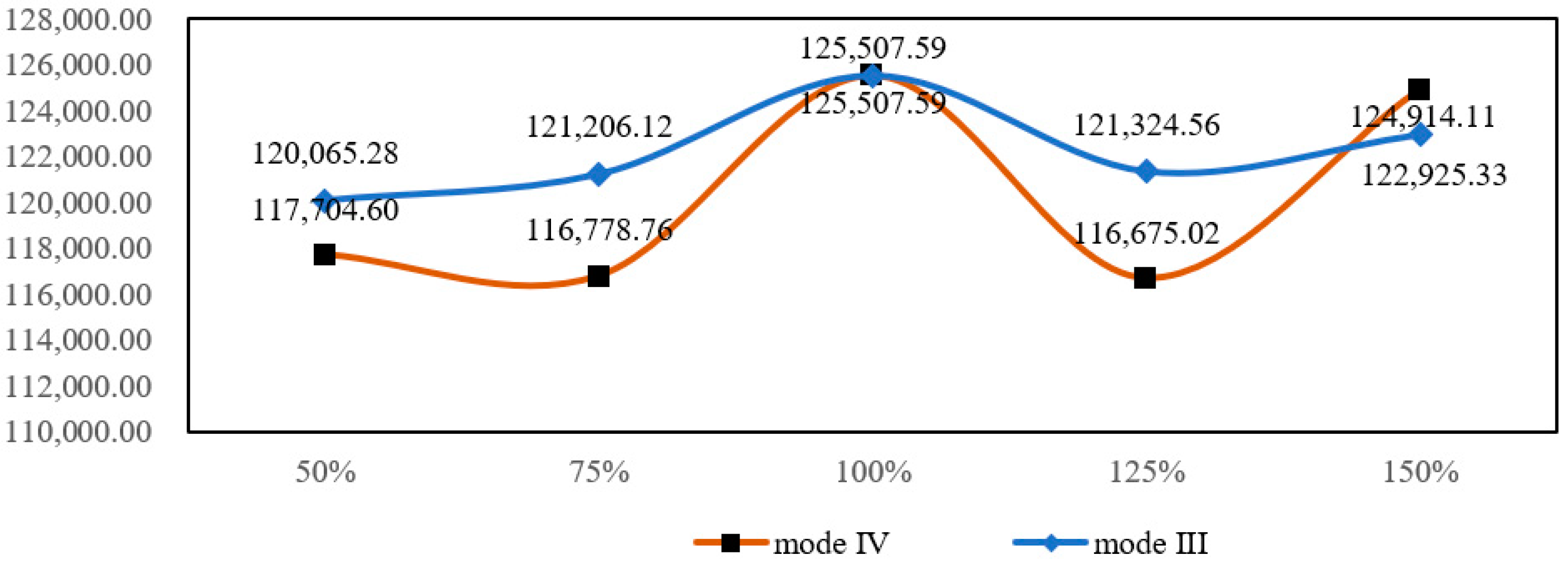
In order to explore the impact of time randomness on cost and decision, the basic value of time variance in models III and IV is changed by 50%, 75%, 125% and 150%, respectively, according to the adjustment ratio in
Figure 5, and the total cost is shown in
Figure 6.
Based on
Figure 6, the impact of time randomness on total cost shows a wave-shaped trend like the ups and downs of the mountains, and there are no obvious laws. The main reason for this phenomenon is that the variance parameter of normal distribution can only restrain the variation degree of time; however, it has obvious randomness for a specific example, and then the total cost associated with time is no longer a non-decreasing linear trend. Nevertheless, some rules and phenomena can still be found from the results. On the one hand, in
Figure 6, the cost change of mode IV (uncertain demand and time) is significantly higher than that of mode III (deterministic demand and uncertain time) under the same degree of time variance, and the fluctuation range is more significant. This further verifies the impact of demand uncertainty. On the other hand, compared with the impact of demand uncertainty in
Figure 5, the impact of time randomness on cost and decision in
Figure 6 is more obvious, and the impact trend is more vague under the same variations. This result suggests that enterprises should pay more attention to the fluctuation of transportation time caused by various reasons.
7. Conclusions
Focusing on the problem of low-carbon multimodal transportation with both demand uncertainty and transportation time randomness, a hybrid robust stochastic optimization (HRSO) model for a multimodal transportation path with dual uncertainty was established, and a catastrophic adaptive genetic algorithm (CA-GA) based on Monte Carlo sampling was designed. On the basis of the algorithm validity, a numerical example analysis was carried out to compare the multimodal transportation scheme and cost under the mode of certainty, demand uncertainty, time randomness and dual uncertainty, and the influence of uncertain parameters was analyzed. Based on the results, the demand uncertainty and time randomness will affect the decision of low-carbon multimodal transportation, not only the transportation path but also the transportation mode. Explicitly, the robust optimization with uncertain demand has a certain conservatism in solving this optimization problem, which will increase the total cost of low-carbon multimodal transportation due to the pursuit of stability. Therefore, it can improve the transportation efficiency of multimodal transportation under an uncertain environment by selecting the appropriate maximum regret value and restricting the relationship between demand uncertainty and total cost. What is more, the randomness of time has a significant and fuzzy influence on the total cost, showing a wavy change trend, like the ups and downs of the mountains, with no obvious law. However, the influence of time randomness on multimodal transportation cannot be ignored.
Overall, our findings can provide some useful insights for the administrative department and logistic services providers to design the transportation scheme. When choosing the transportation path and mode, they should consider the uncertainty of demand and time simultaneously. Note that the methodology, including HRSO model and CA-GA, provides a way to model a low-carbon transportation path under dual uncertainty. Even for the different carbon reduction policies, similar studies can be carried out by adjusting the related parameters. Through a simple modification of the model, more studies on the uncertain low carbon transportation scheme considering different cargo transportation values can also be proposed.
Suggestions for future research include extending the analysis to the constraint ability and influence mechanism of transportation time under dual uncertainty. In addition, due to the complexity of the model construction, the study did not explore the impact of carbon trading price changes on transportation decisions, and establishing a more realistic optimization model will be our next research focus.


