Article

A Bioeconomic Analysis of the Sandfish (Arctoscopus japonicus) Management Policies of the Eastern Sea Danish Fishery in Korea

1
Fisheries Resources Research Division, National Institute of Fisheries Science, Busan 46083, Korea
2
Embassy of the Republic of Korea in Oriental Republic of Uruguay, Montevideo 11300, Uruguay
3
Department of Marine & Fisheries Business and Economics, Pukyong National University, Busan 48513, Korea
*
Author to whom correspondence should be addressed.
Sustainability 2021, 13(14), 7868; https://doi.org/10.3390/su13147868
Submission received: 28 April 2021 / Revised: 5 July 2021 / Accepted: 12 July 2021 / Published: 14 July 2021
(This article belongs to the Special Issue International Fisheries Policy and Economic Analysis)

Abstract

:
Before implementing resource management measures, it is essential to establish the goals of fisheries resource management by assessing the current biomass status and the level of fishing effort. This study aims to compare surplus production models, i.e., process-error and state-space models, based on how they fit the observed data. The effects of the Sandfish Stock Rebuilding Plan are analyzed using a bioeconomic model. The analytical results show that the least error is between the estimated and observed catch per unit effort using the state-space model. Therefore, the analysis results obtained using the state-space model are considered as the most reliable. The total allowable catch for Korean sandfish is set at 2196 tons per year. However, if we increase the current management regulation standard for available annual catch by 50%, the sandfish resource could be depleted. Furthermore, NPV decreased to 172,599 thousand won after ten years, in 2029. Therefore, a recommendation of this study is that when management policies for sandfish stock prioritize recovery, this would facilitate fisheries rebuilding.

1. Introduction

Recently, the need for the management and recovery of fisheries resources has dramatically increased, owing to the declining catch rates by offshore fisheries in Korea. Fisheries resources are shared natural resources, and if they are not fostered and protected, they will deplete rapidly. To manage and protect fisheries resources, seasonal closures, the regulation of size/weight and habitat, as well as total allowable catch (TAC) are currently implemented in Korea. The Korean Fish Stock Rebuilding Plan (KFSRP), launched in 2006, is a comprehensive fisheries management policy aimed at rebuilding and managing the diminishing fisheries resources. Starting with four fish species in 2006, the Korean Ministry of Oceans and Fisheries is currently managing 19 fish species. The results of the pilot projects have shown that the KFSRP could contribute toward increasing the stock of selected species. Therefore, to ensure stable and sustainable business production, effective means of recovering fisheries resources should be established, implemented, and evaluated [1,2,3].
More than 90% of sandfish (Arctoscopus japonicus), one of Korea’s stock rebuilding species, is caught by the Eastern Sea Danish and coastal gillnet fisheries, and it is an important commercial fish species along the east coast. Sandfish has been included in the Fish Stock Rebuilding Plan since 2006, with several stock rebuilding recommendations. Specifically, the proposed recommendations include increasing the catchable length of sandfish (from 11 to 13 cm), extending the seasonal closure to protect immature fish, as well as preventing overfishing by self-regulating the catch amount by the Eastern Sea Danish fishery and restricting the usage of coastal gillnet fisheries fishing gears. Furthermore, using the reserved spawning ground areas efficiently and constructing a spawning ground were added. A legal basis has also been proposed to deter overfishing by tourists’ fish traps near the port area [1]. Additionally, the TAC policy has been implemented by the Eastern Sea Danish fishery since 2009, and the TAC is currently being considered for coastal gillnet fisheries. However, to recover and manage sandfish fisheries resources in the future, it is essential to set and implement an appropriate TAC amount for the Eastern Sea Danish fishery.
To effectively manage fisheries resources, different resource evaluation models should be selected according to the level of available data. It is also necessary to choose a model that can account for uncertainty as much as possible at a given data level and logically explain the resource dynamics. The widely used stock assessment model is the surplus production model because it is easy to calculate and needs the least information. The process error model and the state-space model are the most popular surplus production model.
Recently used stock assessment models include the process-error and state-space models. The process-error model assumes that the error does not occur in the observations, but solely in biomass changes, whereas the state-space model can simultaneously consider the errors occurring in the observed values and biomass changes. Therefore, the process-error model cannot consider uncertainty such as the one on data collection. However, the state-space model can deal with both errors simultaneously, which is beneficial for reducing uncertainty. For effective fisheries resource management, the most reliable stock assessment model should be selected through comparative analyses of various resource evaluation models [4]. For example, sandfish resources are assessed using a process-error model [5,6]. A recent study conducted by the National Institute of Fisheries Science used a process-error model to estimate the maximum sustainable yield (MSY) of this species and reported it to be 4489 tons [7]. Moreover, these models have a drawback in that they consider only the process errors generated by fishery biomass dynamic functions and are unable to evaluate observation errors occurring from the collective data [8]. Moreover, a recent study has found that the difference between the actual and estimated catch per unit effort (CPUE) with the process-error model is significant, while, for the state-space model, the error between the nominal and estimated CPUE is small. Nonetheless, the root mean square error (RMSE) analysis results for comparing the fit of each model have been found to best reflect the changes in observed values [9,10].
Therefore, for practical resource appraisal, it is necessary to compare various resource assessment models. Moreover, analyses on the effect of each fisheries management scheme are essential for better stock management, and those should include social and economic aspects. Thus, the bioeconomic model should be utilized, which can assess fisheries management schemes both for biological effect (e.g., change on biomass or catch volume) and economic effect (change on fisheries income) [11,12,13,14].
This study aims to compare surplus production models, i.e., process-error and state-space models. We (1) conduct a practical resource assessment on a resource management system that lacks data for resource evaluation and management despite resource recovery; (2) compare the results of the process-error model [15,16], which assumes that the error ensues from biomass changes, and the state-space model [17,18,19], which simultaneously considers the observation and process errors; and (3) analyze the effects of possible stock rebuilding measures for sandfish fishery (such as TAC and fishing effort regulation) and the adequate annual TAC quantities to present appropriate TAC quantities using the bioeconomic modeling technique.
We intend to select the most realistic model for effective sandfish resource management through a comparative analysis of the process-error and state-space models. Using the selected evaluation model results, we analyze the biological and socioeconomic effects of each fisheries management plan.

2. Materials

2.1. Sandfish Fishing Status

Figure 1 shows the sandfish catch amount from the East Sea from 1958 to 2019 [20]. The highest yield was 24,809 tons in 1971, and the lowest was 1286 tons in 2001. In 2019, it decreased to 3066 tons (Figure 1).
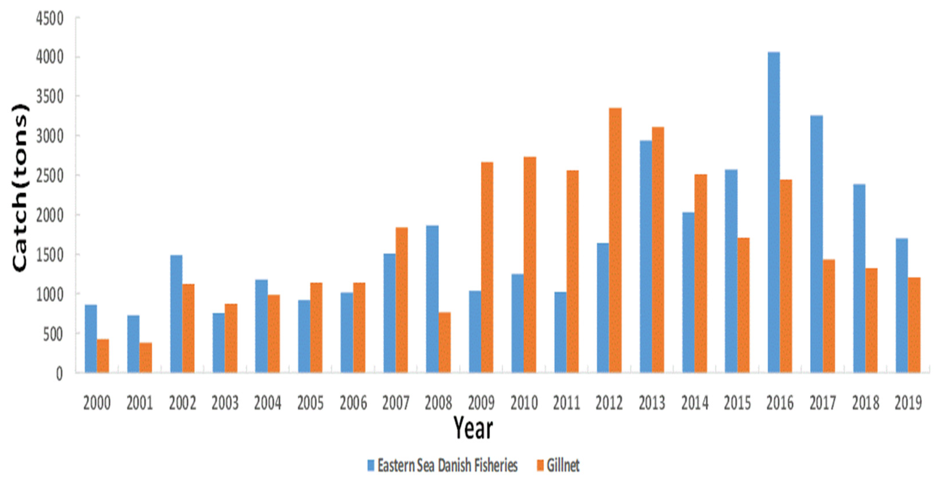
Figure 2 shows the sandfish catch amount by the coastal gillnet and Eastern Sea Danish fisheries since 2000. The catch amount of sandfish by the Eastern Sea Danish fishery started at 868 tons in 2000 and was 1705 tons in 2019, while that by the coastal gillnet fishery started at 427 tons in 2000 and was 1209 tons in 2019 (Figure 2).
Eastern Danish fishery (boat seiners) and coastal gill net fishery are based on the Eastern coast of Korea. The former is one of the leading fisheries on the Eastern coast, and the main target species are sandfish, flounder, herring, common squid, and shrimps prevalent in the Korean market. Coastal gill net fishery mainly fishes on the area with sand sediment with a depth of 150 m to 300 m. It usually catches sandfish, herring, and anchovy. The fishery accounting for the highest percentage of sandfish catches was the Eastern Sea Danish fishery (boat seiners) with approximately 57%, followed by the coastal gillnet fishery (set gill nets) with 32% and others with 10%. In this study, the analysis focuses on the Eastern Danish fishery, which is managed with TAC and catches the most considerable amount of sandfish.

2.2. Data Analysis

Table 1 presents the sandfish catch amount and effort by the Eastern Sea Danish fishery since 2004, when their effort data became available [20]. In this study, horsepower (HP), which has the highest statistical significance among the number of vessels and tonnage, is used as a fishing effort index. Sandfish catch amount started at 1183 tons in 2004 and reached 1705 tons in 2019. The catch effort (HP) began at 16,914 HP in 2004 and reached 17,796 HP in 2019 [20]. The number of Eastern Danish vessels under TAC was 42 in 2004, but it declined to 39 in 2019. However, total horsepower increased from 16,914HP to 17,796 HP in the same period [20]. That means horsepower, a critical variable for this fishery’s fishing pressure, increased even though the number of vessels decreased with the government’s buy-back program [1]. Thus, this study utilized horsepower as the indicator of fishing effort, which also has the most statistical significance.
The total fishing cost and market price data for the Eastern Sea Danish fishery are used to analyze the bioeconomic model and obtain the Eastern Sea Danish fishery’s cost status. The labor cost (50%) is the highest, followed by production management cost (28%), other miscellaneous expenses (10%), selling and administrative expenses (6%), and depreciation expenses (6%) [21]. Based on the Fisheries Information Service data, the average unit price of sandfish from 2016 to 2018 was 1345 won per kg [22]. For the analysis method, please refer to the Appendix A.

3. Results

3.1. Process-Error Model

The fit of the CYP model, which is a process-error model, is statistically significant. Moreover, the adjusted R2 value for the model is 57%. Lastly, the sign of the coefficients is as expected (F = 10.41, p-value = 0.002385).

3.2. State-Space Model

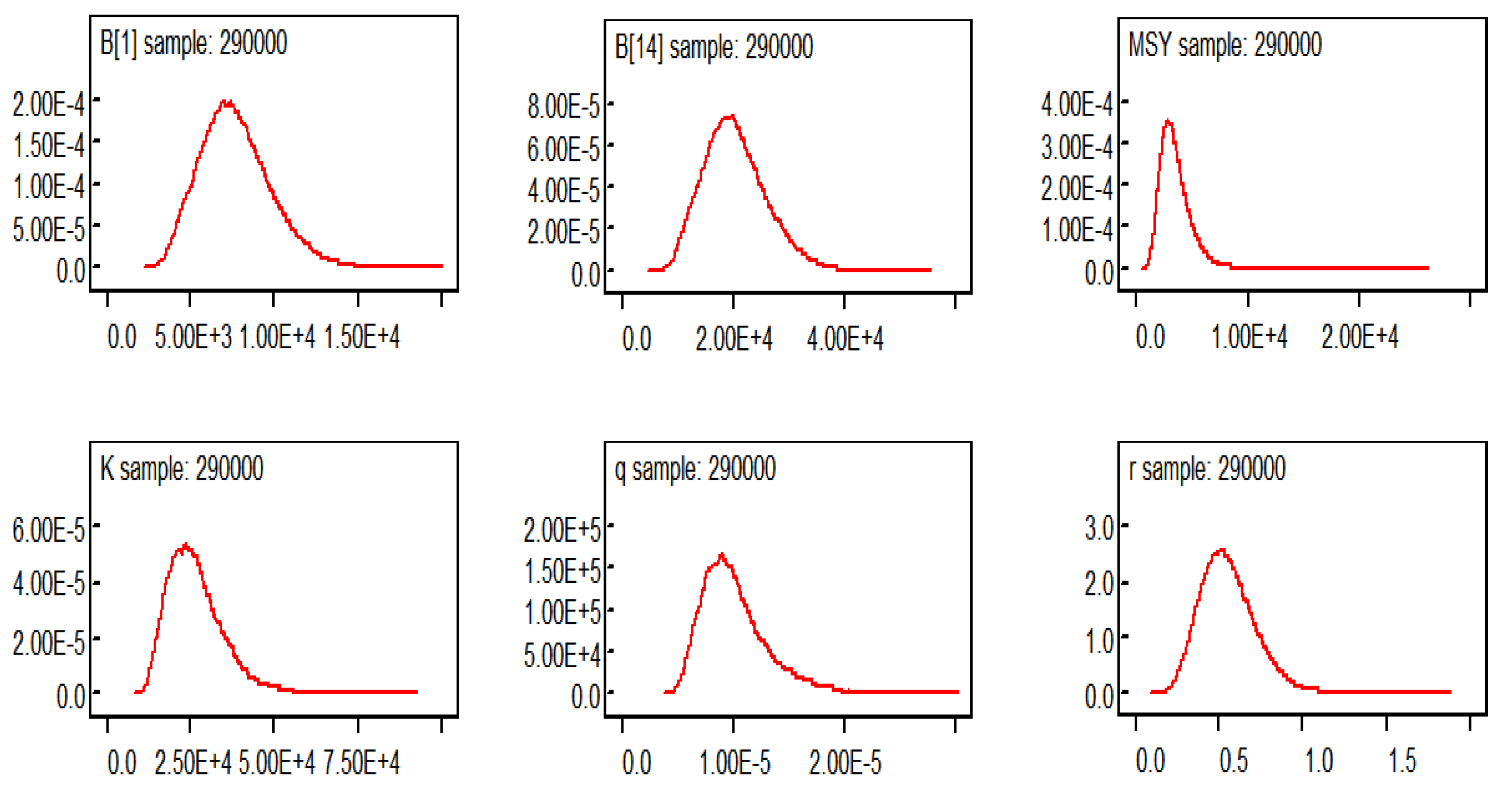
The state-space model is derived using the WinBUGS (Bayesian inference using Gibbs sampling) program, which specializes in Bayesian inference using Gibbs sampling [23,24]. To analyze the model, 300,000 specimens are extracted. Among them, the initial 10,000 samples that were not consistent with the posterior distribution were discarded by setting the burn-in period. Furthermore, the 29th sample was extracted to minimize sample correlation that was observed during the extraction process. Finally, the posterior distribution was derived using 10,000 samples. One of the verification methods of the state-space model is that the model is determined to be appropriate if the estimates of variables from checking the trial table do not show a particular form or tendency, i.e., they have a white noise form. Based on the trial table of the critical variables, such as B (biomass), r (intrinsic growth), q (catchability coefficient), K (carrying capacity), and MSY (maximum sustainable yield,) which have a white noise form, i.e., do not show a particular form, the state-space model for sandfish is reasonably evaluated (Figure 3 and Figure 4).
If the estimated variable’s Monte Carlo error is less than 5% of the post-standard error, it can be established that the model is appropriate. The Monte Carlo error of all variables estimated using the state-space model is 5%; therefore, the model is adjudged to be suitable [25] (Table 2).

3.3. Comparison of Analysis Results Obtained Using the Model

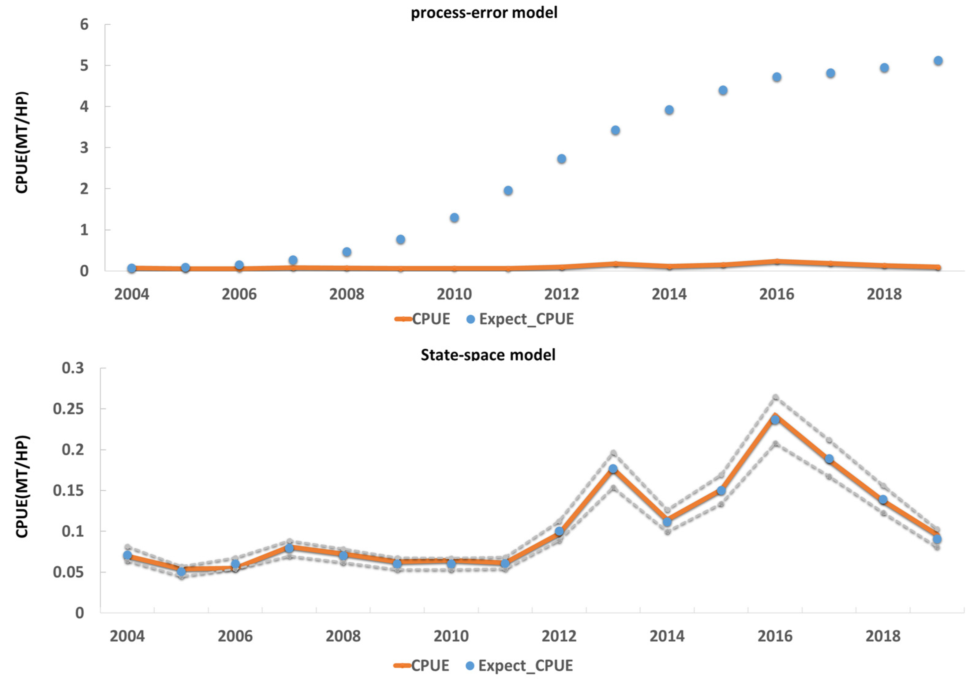
We compare the actual annual and estimated CPUEs by posterior distribution using the process-error and state-space models. In the process-error model, the error range between the actual and estimated CPUE is extensive. Conversely, the estimated CPUE with the Bayesian state-space model seems to reflect the actual CPUE relatively better (Figure 5).
In the state-space model, the correlation between the parameters can be reduced by reconstructing the resource amount as a ratio of itself to the environmental capacity [17]. It is also possible to reduce the uncertainty in parameter estimation by the pre-distribution of parameters set in the estimation process [26]. Furthermore, by estimating each parameter’s distribution, the extent of the change owing to the correlation of the parameters can be obtained. The estimated results of the state-space model are as follows: the 97.5% confidence interval range of sandfish parameters includes the MSY) of 1391–6500 tons, K of 15,600–53,200 tons, q of 0.0000051–0.0000148, and r of 0.20 to 0.76. The results obtained using the process-error model are as follows: the MSY is 9820 tons, K is 68,631 tons, q is 0.00009, and r is 0.38.
The RMSE and R2 values of the CPUE error are estimated to compare and analyze the two models. The RMSE values are 3.023 for the process-error model and 0.0029 for the state-space model, while the R2 values are 0.57 for the process-error model and 0.99 for the state-space model (Table 3).

3.4. Analysis of the Effect of Sandfish Stock Rebuilding

Based on the above-mentioned analysis, a bioeconomic model is constructed using the variables of the state-space model. Thereafter, we analyze the effect of the TAC and fishing effort limit spectrum on sandfish resources. To analyze the effects of stock rebuilding measures for sandfish fishery, we divide the TAC range setting into +50%, +30%, −30%, and −50% based on the TAC volume of 2196 tons. The fishing effort is divided into +60%, +50%, +30%, −30%, and −50% based on the Eastern Sea Danish fishery effort of 17,796 HP.
In the analysis of substantial effects, the period is set to 2029, 10 years after the stock rebuilding period. The biological effects of the stock rebuilding measures are assessed as changes in the biomass. The economic effects are evaluated as income changes in the Eastern Sea Danish fishery. Here, the fishery import price is the market price (p) multiplied by the catch amount of sandfish in year t, evaluated using the production function ( H t ) as in Equation (A22). Over the next ten years, fishing revenue is calculated based on the NPV, assuming a 4.5% social discount rate ( δ ), as shown in Equation (A24) (Table 4).
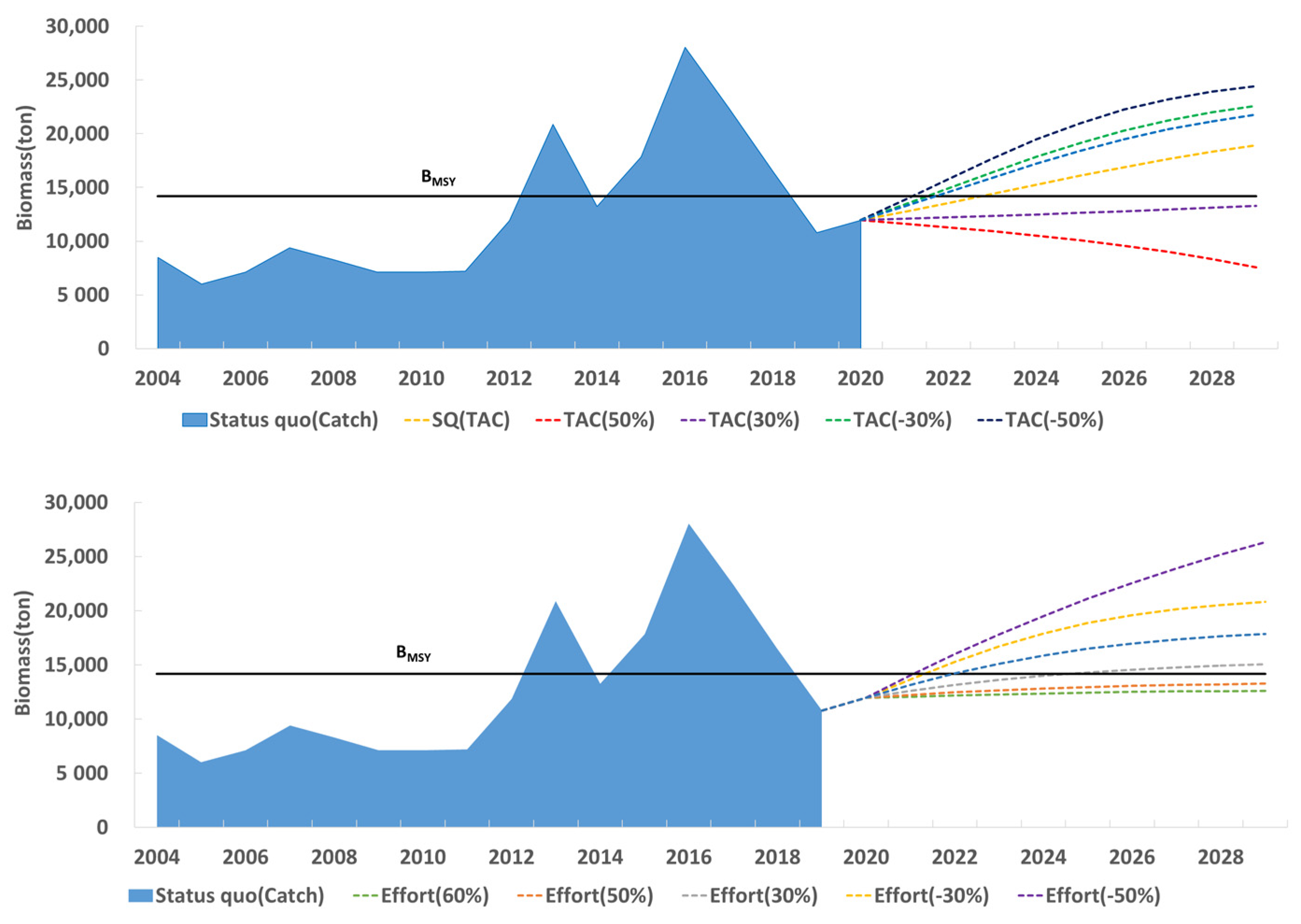
The biological effect is evaluated based on a comparison between the current catch level and TAC level. Suppose the TAC is set at 2196 tons, as in the present scenario, the biomass increases. If the TAC is reduced by 50%, the future biomass grows to be the highest at 24,446 tons.
The economic effect is evaluated as the NPV of 246,462 thousand won when the TAC is set at 2196 tons. The analysis of the impact of fishing effort changes shows that increasing fishing effort by 60% at the current level could decrease the NPV and reduce future resources to 12,590 tons. However, reducing the fishing effort to −30% increases the future biomass to 20,815 tons, while the NPV increases above the status quo (Figure 6).

4. Discussion

Sandfish is included in the 2006 Stock Rebuilding Plan. It is a representative fish species whose resources have been successfully recovered through budgets, human resources, government, and fishermen’s efforts. However, the sandfish fisheries resource, which has been recovering from hitherto overexploitation, is in danger of declining. This study aims to compare the stock assessment models currently being used to evaluate practical sandfish fisheries resources and propose a plan for selecting and applying effective stock assessment models. We also attempt to assess the optimal resource management method by analyzing each resource tool’s effect to choose a useful resource evaluation model.
The catch amount of sandfish has declined since 2017, as shown in Figure 1. However, the current stock assessment of sandfish in Korea still solely relies on the process-error model. For example, sandfish resources have been assessed using the process-error model [5,6]. This study reveals the gap between the actual and estimated CPUEs using the process-error model. Conversely, the estimated CPUE with the Bayesian state-space model seems to reflect the actual ones relatively better. Thus, in this study, we compare various stock assessment models.
A reasonable stock assessment model is selected by analyzing the process error and state-space models. In the process-error model, the MSY level is 9820 tons, K is 68,631 tons, q is 0.00009, and r is 0.38. In the state-space model, the MSY level is 3031 tons, K is 14,190 tons, while q and r are 0.000008 and 0.42, respectively. To compare and analyze the two models, we evaluate the RMSE and R2 values of the CPUE error. For the process-error model, the RMSE and R2 values are 3023 and 0.57, respectively, while for the state-space model, the RMSE and R2 values are 0.0029 and 0.99, respectively.
To analyze the effects of the sandfish resource management measures, we construct a bioeconomic model using the state-space model’s estimates and investigate its biological and economic effects. Upon analysis using the current level and TAC quantity, it is shown that if the TAC volume is set at 2196 tons, as it is currently, the biomass increases. When the set TAC decreases by 50%, the assessed biomass is the highest at 26,321 tons, and when the economic effect reduces to −30%, the NPV is evaluated to be the largest at 164,140,000 won.
The fishing effort analysis reveals that the NPV increases when −30% of the fishing effort decreases at the current level. It is estimated that the biomass would increase to 16,140 tons in the future; however, if the fishing effort increases to 50%, the future biomass decreases to 13,273 tons, and the NPV also decreases.
According to the Korean fish stock rebuilding plan, the rebuilding target is set to BMSY. This study analyzed that when the rebuilding target for sandfish biomass is set to BMSY of 14,190 tons if the TAC quota is reduced by 30% from the current level, the sandfish biomass recovers to 14,899 tons in 2022 to the rebuilding target level
It has been shown that the increase in TAC setting by more than 30%, compared to the current level, or the increase in the level of catch effort by 30%, compared to the current status, adversely affects resources. Therefore, when setting the TAC and fishing effort in the future, it should not be assigned more than a 30% increase relative to the current level.
The rebuilding target is set to BMSY according to the KFSRP. Table 4 shows that the MSY estimated by the state-space model is 3031 tons, which is higher than both the current catch and TAC levels. It is desirable that the TAC setting for rebuilding should be set lower than the MSY, which is crucial when considering various factors. Based on the result that the current biomass is lower than the BMSY, to recover to the rebuilding target level, the current catch must be set lower than the MSY level.
Process errors occur when the stock assessment model’s assumptions do not reflect changes in fisheries resources and observation errors owing to the lack of collected observation data. For example, the surplus production model used in this study assumes that the r of the fish population is constant. However, in reality, the internal production rate of fisheries resources changes every year due to various internal and external environmental factors. Furthermore, CPUE, the primary observational data used in the surplus production model, does not fully reflect the change in the actual biomass due to various factors, such as changes in the fishing environment and data uncertainties. Accordingly, if a stock assessment is performed using statistical techniques that can reflect such uncertainties, more realistic results can be derived [9,10]. This study shows that the state-space model, which considers both process and observation errors, is the most suitable.
Until now, the process-error model has been used the most in TAC calculation and fisheries resource evaluation in Korea [27,28,29,30]. Previous research on the assessment of sandfish resources has utilized the process-error model solely to analyze the effect of TAC [31]. However, this study employs the Bayesian state-space model to obtain the most effective fishing effort reduction scheme and investigate the effect of TAC. An economic feasibility analysis is necessary with the Bayesian state-space model’s estimation, as this study does, because the uncertainty of the process-error model is considerable, as stated in previous research. Moreover, TAC and other resource management measures should be effectively implemented.
Previous research has focused on the comparison of effort-averaging methods, the process-error model, and the observation-error model [32]. The observation-error model has been found to be the most appropriate for stock assessment. This means that it does not consider the state-space model, which can simultaneously include both process and observation errors. However, [17] included a state-space model for stock assessment. The results show that the parameter is most similar to that of the observation-error model [32]. Thus, the state-space model is more useful for accurate stock assessment. Moreover, in the case of sandfish, the target species of this study, the state-space model that can consider both process and observation errors is found to be the most suitable, which is the same as the results of previous studies [9,10].
In the analysis of the socioeconomic effectiveness of fisheries management, it is found that the economic effect is the greatest when the TAC is set at 2500 tons of sandfish, as presented in the previous study [31]. Conversely, in this study, it is found that the most significant economic effect appears at the current catch (2196 tons). The biological effectiveness analysis, similar to the results of previous studies, shows that the TAC setting of 1500 tons is analyzed to most significantly increase the fish biomass.
Furthermore, the state-space model requires the assumption of a prior distribution. In the case of sandfish, the prior distribution is set based on previous stock assessment information [5,6]. Because there was a prior distribution appropriate for sandfish in previous research, uncertainty from the prior distribution was eliminated. If not, the uncertainty of the state-space model is not so different from that of the process error model. However, other fish species that do not have previous stock assessments would face great difficulty in setting the prior distribution. In this regard, reference points for prior distribution settings for fish stock without stock assessment should be subsequently introduced.
In this study, we conduct a stock assessment with only the Eastern Sea Danish fishery, which has the highest sandfish fishing rate and the most catch effort data. However, sandfish assessment without considering other fisheries, such as the gillnet fishery, with the second-highest fishing rate of 32%, remains a limitation that ensues from a lack of effort data. Future sandfish assessment, including gillnet fisheries data, enables the analysis of the necessary policy data for a more accurate estimate [33,34].
Therefore, to increase the sandfish fisheries resources, a useful stock assessment model should be selected. The optimal means of recovering fisheries resources should be sought by analyzing the effects of stock rebuilding strategies for sandfish fishery. In this study, the state-space model was more suitable to evaluate and rebuild the sandfish stocks, comparing to the process error model. In addition, the result of effect analysis on the fishery stock rebuilding strategies using state-space model, reveals that setting over 30% of current TAC as next level can be adversely affected to the stock. Therefore, to ensure stable and sustainable business production, effective means of recovering fisheries resources should be established, implemented, and evaluated. Moreover, the effects of the measures of recovering fisheries resources should be analyzed to promote the actual recovery and management of fisheries resources

Author Contributions

Conceptualization, J.-H.C. and D.-H.K.; methodology, J.-H.C. and D.-H.K.; software, J.-H.C.; validation, J.-H.C. and D.-H.K.; formal analysis, J.-H.C.; investigation, D.-H.K.; resources, J.-H.C. and D.-H.K.; data curation, J.-H.C. and D.-H.K.; writing—original draft preparation, J.-H.C. and S.-C.Y.; writing—review and editing, J.-B.L. and S.-C.Y.; visualization, J.-H.C. and S.-C.Y.; supervision, J.-B.L. and S.-C.Y.; project administration, J.-B.L. and S.-C.Y.; funding acquisition, S.-C.Y. All authors have read and agreed to the published version of the manuscript.

Funding

This study was supported by a grant from the National Institute of Fisheries Science (R2021069).

Institutional Review Board Statement

Not applicable.

Informed Consent Statement

Not applicable.

Data Availability Statement

Publicly available datasets were analyzed in this study. This data can be found here: https://kosis.kr/ (accessed on 18 January 2020).

Conflicts of Interest

The authors declare no conflict of interest.

Appendix A

Appendix A.1. Methods

Appendix A.1.1. Surplus Production Model

The resource dynamics model (surplus production model) combines biomass, growth, and natural mortality with the concept of surplus production. The resource dynamics are defined as follows:
                  B y + 1 = B y + g ( B y ) C y
In the above-stated Equation (A1), B y is the biomass in year y, g ( B y ) is the surplus production function of biomass, and C y is the catch amount of year y. Here, the type of resource dynamics model is determined based on the assumptions of the natural surplus production function:
g ( B y ) = r B y ( 1 B y K )  
g ( B y ) = r B y l n ( K ) [ 1 ( ln ( B y ) ln ( K ) ) ]  
    g   ( B y ) = r p B y [ 1 ( B y K ) P ]  
where r is the intrinsic growth rate of fisheries resources, K is the carrying capacity, and p is a parameter that determines the type of growth function. Among the surplus production functions, Equation (A2) is devised by [35] as a function of the logistic model (Schaefer model), Equation (A3) is proposed by [36] as a function of the exponential model (Fox model), and Equation (A4) is a growth function devised by [37] (Pella and Tomlinson model).
B y + 1 = B y + r P B y [ 1 ( B Y K ) P ] C y
In the surplus production model, the relationship between fishing efficiency and resource quantity is assumed to be constant [23]. The function of the observed value of the resource can be expressed as Equation (A6).
I y = q B y
In Equation (A6), I y is the CPUE and q is the catchability coefficient. The above-stated dynamic model can be estimated using the process-error, observation-error, and state-space models.

Appendix A.1.2. Process-Error Model (CYP Model)

The process-error model assumes that an error does not occur in the observed value. However, an error occurs only in the biomass, and the biomass is estimated using a linear regression model [32]. In particular, five models [15,16,35,36,37,38] have been mainly used in the evaluation of fisheries resources in Korea. In this study, the Clarke–Yoshimoto–Pooley (CYP) model with the highest statistical significance among the five models is used for the analysis.
In this study, we apply the CYP model, which is estimated to be the best fit among the process-error models. To estimate the CYP model, if Equation (A3) is differentiated with respect to y and is multiplied by q/I, Equation (A7) can be calculated.
( 1 / I ) d I / d y = r l n ( q K ) r l n ( I ) q E
If Equation (A7) is an integral from year n to year n+1, it can be expressed as Equation (A8) as follows:
l n ( I n + 1 I n ) = r l n ( q K ) r y = n n + 1 l n ( I ) d y q E n ¯
where I n is the CPUE at the beginning of the year and E n ¯ is the represents fishing effort of year n. The first-order Taylor polynomial for the above-stated function can be represented by Equation (A9):
l n ( I ) = I n ( I ¯ n ) + 1 I ¯ n ( I I ¯ n )  
Integrating Equation (A9) can be expressed as Equation (A10):
n n + 1 I n ( I ) d y = I n ( I ¯ n ) 1 + 1 I ¯ n n n + 1 I d y
By substituting Equation (A10) into Equation (A8), Equation (A11) can be calculated as:
l n ( I n + 1 I n ) = r I n ( q K ) r l n ( I ¯ n ) q E ¯ n
If n + 1 is substituted for n in Equation (A11), Equation (A12) can be calculated as:
l n ( I n + 1 I n ) = r I n ( q K ) r l n ( I ¯ n + 1 ) q E ¯ n + 1
If Equations (A11) and (A12) are combined, Equation (A13) is expressed as:
l n ( I n + 2 I n + 1 I n + 1 I n ) = 2 r I n ( q K ) r [ ln ( I ¯ n ) + l n ( I ¯ n + 1 ) ] q ( E ¯ n + E ¯ n + 1 )  
If the assumption ( I ¯ n = I n + 1 I n ) from (A8) is applied to Equation (A13), the relation for assuming the CYP model can be derived as:
l n ( I ¯ n + 1 ) = 2 r 2 + r ln ( q K ) + 2 r 2 + r ln ( I ¯ n ) q 2 + r ( E ¯ n + E ¯ n + 1 )  

Appendix A.1.3. State-Space Model

In the state-space model, the biomass ( B y ) is reconstructed using the ratio of the biomass to K ( P y = B y / K ), and the error is assumed to follow a lognormal distribution [39].
P 1 σ 2 = e u 0 P y P y 1 ,   K ,   r ,   σ 2 = ( P y 1 + r P y 1 ( 1 P y 1 ) C y 1 K ) e u y
I y P y ,   q ,   τ 2 = q K P y e u y
Based on the references for the prior distribution [17,24,40], an informative prior distribution is assumed for r and K; lognormal and inverse-lognormal distributions are set for r and K, respectively. For q, the inverse-gamma distribution is set as a non-informative prior distribution. The average value of the informative prior distribution is referred to in [6,7].
p ( K ,   r ,   q , σ 2 ,   τ 2 , P 1 ,   ,   P N ) = p ( K ) p ( r ) p ( q ) p ( σ 2 ) p ( τ 2 ) p ( p 1 σ 2 ) × Y = 1 N p ( P y + 1 P y ,   K ,   r ,   σ 2
The probability that the CPUE is observed when a biological coefficient has a specific value can be expressed as follows:
p ( I 1 ,   ,   I N K ,   r ,   q ,   σ 2 ,   τ 2 ,   P 1 ,   ,   P N ) = y = 1 N p ( I y p y ,   q ,   τ 2 )
According to Bayes’ theorem, the posterior distribution can be estimated using the prior probability Equations (A12) and (A13).
p ( K ,   r ,   q , σ 2 ,   τ 2 , P 1 ,   ,   P N ,   I 1 ,   ,   I N )   = p ( K ) p ( r ) p ( q ) p ( σ 2 ) p ( τ 2 ) p ( p 1 σ 2 ) × y = 2 N p ( P y P y 1 , K ,   r ,   σ 2 ) y = 1 N p ( I y P y ,   q ,   τ 2 )

Appendix A.1.4. Model Test

Because it is difficult to determine the parameters for fisheries resources, it is quite challenging to assess which model reflects the most accurate estimates. As an alternative to overcoming these problems, we compare and analyze the difference between the estimated value in the model and the actual data [41,42].
To assess the extent to which the estimated quantity of fish per unit effort ( I y ) per year, as estimated by each model and actually reflects the observed amount of fish per unit effort ( I ^ y ), the RMSE and coefficient of determination ( R 2 ) of the error are calculated as follows:
R M S E = 1 n y ( I y I y ^ ) 2
R 2 = 1 y ( I y I y ^ ) 2 y ( I y I ¯ ) 2 ; I ¯ = 1 n = y I y

Appendix A.1.5. Economic Analysis

The average market price of sandfish caught by the Eastern Sea Danish fishery from 2015 to 2017 multiplied by the sandfish catch amount can be represented using Equation (A22):
T R y = H y · p
Fishery costs can be expressed using Equation (A23) as the product of HP and the average cost per HP used in the harvest of the species by using the results of management surveys conducted by the Eastern Sea Danish fishery in the past three years:
T C y = C · H P y
Suppose fishery cost is deducted from fishery income; thus, fishery profit can be obtained, and the sum of yearly fishery profit that would occur in the next ten years, assuming a 4.5% social discount interest rate, can be expressed as Equation (A24). The interest rate was applied to calculate the present value, as the General Guideline for Preliminary Feasibility Assessment (https://www.kdi.re.kr/) recommended to calculate the present value.
N P V ( n e t   p r e s e n t   v a l u e ) = y = 1 10 ( T R y T C y ) ( 1 + i ) t

References

  1. Ministry of Oceans and Fisheries. Report of Fish Stock Rebuilding Plan Regional Scientific Committee; Ministry of Oceans and Fisheries: Sejong, Korea, 2020.
  2. Lee, S.G.; Midani, A.R. National comprehensive approaches for rebuilding fisheries in South Korea. Mar. Policy 2014, 45, 156–162. [Google Scholar] [CrossRef]
  3. National Institute of Fisheries Science. Target Fish Species of Fisheries Resources Recovery Project. Available online: https://www.nifs.go.kr/page?id=rec_fish (accessed on 15 February 2020).
  4. Kim, D.Y.; Lee, J.S.; Kim, D.H. A study on establishing the performance evaluation system of the fish stock rebuilding plans. J. Fish. Bus. Adm. 2011, 42, 15–29. [Google Scholar]
  5. Lee, S.I.; Yang, J.H.; Yoon, S.C.; Chun, Y.Y.; Kim, J.B.; Cha, H.K.; Choi, Y.M. Biomass estimation of sailfin sandfish in Korea waters. Korean J. Fish Aquat. Sci. 2009, 42, 487–493. [Google Scholar]
  6. Choi, J.Y.; Kim, D.H. An exploratory study on determining optimal fishing effort and production levels of danish seine fishery under the sandfish stock rebuilding plan. J. Fish. Bus. Admin. 2012, 43, 1–9. [Google Scholar] [CrossRef] [Green Version]
  7. National Institute of Fisheries Science. Resource Status and Restoration Recommendation of Fisheries Resources in 2017; National Institute of Fisheries Science: Busan, Korean, 2017.
  8. Choi, M.J.; Kim, D.H. Assessment and management of small yellow croaker (Larimichthys polyactis) stocks in South Korea. Sustainability 2020, 12, 8257. [Google Scholar] [CrossRef]
  9. Choi, M.J. Comparing surplus production models for selecting effective stock assessment model: Analyzing potential yield of East Sea, Republic of Korea. Ocean Polar Res. 2019, 41, 183–191. [Google Scholar]
  10. Choi, M.J. A bioeconomic Analysis of Small Yellow Croaker for Planning Effective Management Policy. Master’s Thesis, Pukyong National University, Busan, Korea, 21 February 2020. [Google Scholar]
  11. Larkin, S.; Alvarez, S.; Sylvia, G.; Harte, M. Practical considerations in using bioeconomic modelling for rebuilding fisheries. OECD Food Agric. Fish. 2011, 1–38. [Google Scholar] [CrossRef]
  12. Clark, C.W. Mathematical Bioeconomics: The Optimal Management of Renewable Resources; John Wiley & Sons, Inc.: New York, NY, USA, 1990. [Google Scholar]
  13. Clark, C.W. Fisheries bioeconomics: Why is it so widely misunderstood? Popul. Ecol. 2006, 48, 95–98. [Google Scholar] [CrossRef]
  14. Davis, J.C. Rebuilding fisheries: Challenges for fisheries managers. In The Economics of Rebuilding Fisheries Workshop Proceedings; OCED: Paris, France, 2010; pp. 1–270. [Google Scholar]
  15. Schnute, J. Improved estimates from the Schaefer production model: Theoretical considerations. J. Fish. Board Can. 1977, 34, 583–603. [Google Scholar] [CrossRef]
  16. Clarke, R.; Yoshimoto., S.; Pooley, S. A bioeconomic analysis of the Northwestern Hawaiian Islands lobster fishery. Mar. Resour. Econ. 1992, 7, 115–140. [Google Scholar] [CrossRef]
  17. Millar, R.B.; Meyer, R. Non-linear state space modelling of fisheries biomass dynamics by using Metropolis-Hastings within-Gibbs sampling. J. R. Stat. Soc. C Appl. 2000, 49, 327–342. [Google Scholar] [CrossRef]
  18. de Valpine, P.; Hilborn, R. State-space likelihoods for nonlinear fisheries time-series. Can. J. Fish. Res. Board Can. 2005, 62, 1937–1952. [Google Scholar] [CrossRef]
  19. Winker, H.; Carvalho, F.; Kapur, M. JABBA: Just another Bayesian biomass assessment. Fish. Res. 2018, 204, 275–288. [Google Scholar] [CrossRef]
  20. Korean Fisheries Information Service. Fishery Production Statistics. Available online: http://fips.go.kr (accessed on 18 January 2020).
  21. Korea Fisheries Resources Agency. Coastal Fisheries Survey Report; FIRA-ER-17-018: Busan, Korea, 2017; pp. 307–311. [Google Scholar]
  22. Korean Statistical Information Service. Korean Statistical Information Service. Available online: http://kostat.go.kr (accessed on 18 January 2020).
  23. Haddon, M. Modelling and Quantitative Methods in Fisheries; CRC Press: New York, NY, USA, 2010; pp. 285–333. [Google Scholar]
  24. Kim, D.H. Bayesian Statistics Using R and WinBUGS; Freedom Academy: Paju, Korea, 2013; pp. 87–248. [Google Scholar]
  25. Spiegelhalter, D.J.; Thomas, A.; Best, N.; Lunn, D. WinBUGS User Manual. 2003. pp. 1–60. Available online: https://www.mrc-bsu.cam.ac.uk/wp-content/uploads/manual14.pdf (accessed on 15 March 2020).
  26. McAllister, M.K.; Pikitch, E.K.; Punt, A.E.; Hilborn, R. A Bayesian approach to stock assessment and harvest decisions using the sampling/importance resampling algorithm. Can. J. Fish. Aquat. Sci. 1994, 51, 2673–2687. [Google Scholar] [CrossRef]
  27. Zhang, C.I.; Kim, S.; Yoon, S.B. Stock assessment and management implications of small yellow croaker in Korean waters. Korean J. Fish. Aquat. Sci. 1992, 25, 282–290. [Google Scholar]
  28. Choi, Y.M.; Zhang, C.I.; Lee, J.B.; Kim, J.Y.; Cha, H.K. Stock assessment and management implications of chub mackerel, Scomber japonicus in Korean waters. Korean J. Fish. Aquat. Sci. 2004, 6, 90–100. [Google Scholar]
  29. Sohn, M.H.; Yang, J.H.; Park, J.H.; Lee, H.W.; Choi, Y.M.; Lee, J.B. Stock assessment and optimal catch of blackfin flounder Glyptocephalus stelleri in the East Sea, Korea. Korean J. Fish. Aquat. Sci. 2013, 46, 598–606. [Google Scholar]
  30. Sim, S.H.; Nam, J.O. A stock assessment of yellow croaker using bioeconomic model: A case of single species and multiple fisheries. Ocean. Polar Res. 2015, 37, 161–177. [Google Scholar] [CrossRef]
  31. Kim, D.H. Evaluating the TAC policy in the sandfish stock rebuilding plan. J. Fish. Bus. Admin. 2015, 46, 29–39. [Google Scholar] [CrossRef]
  32. Polacheck, T.; Hilborn, R.; Punt, A.E. Fitting surplus production models: Comparing methods and measuring uncertainty. Can. J. Fish. Aquat. Sci. 1993, 50, 2597–2607. [Google Scholar] [CrossRef]
  33. Christou, M.; Maynou, F.; Tserpes, G.; Stergiou, K.I.; Maravelias, C.D. Crash landing obligation for Mediterranean mixed fisheries: Evaluation of management strategies using bioeconomic modelling in the Aegean Sea. Sci. Mar. 2019, 83, 143–154. [Google Scholar] [CrossRef] [Green Version]
  34. Sgardeli, V.; Tserpes, G.; Maravelias, C.D. Optimizing effort allocation in data poor mixed fisheries. ICES J. Mar. 2019, 76, 1505–1514. [Google Scholar] [CrossRef]
  35. Schaefer, M.B. Some aspects of the dynamics of populations important to the management of the commercial marine fisheries. IATTC Bull. 1954, 1, 23–56. [Google Scholar]
  36. Fox, W.W. An exponential surplus-yield model for optimizing exploited fish populations. Trans. Am. Fish. Soc. 1970, 99, 80–88. [Google Scholar] [CrossRef]
  37. Pella, J.J.; Tomlinson, P.K. A generalized stock production model. IATTC Bull. 1969, 13, 416–497. [Google Scholar]
  38. Walters, C.J.; Hilborn, R. Adaptive control of fishing systems. J. Fish. Res. Board Can. 1976, 33, 145–159. [Google Scholar] [CrossRef]
  39. Meyer, R.; Millar, R.B. BUGS in Bayesian stock assessments. Can. J. Fish. Aquat. Sci. 1999, 56, 1078–1087. [Google Scholar] [CrossRef]
  40. Punt, A.E.; Hilborn, R. Bayesian Stock Assessment Methods in Fisheries: User’s Manual; Food and Agriculture Organization: Rome, Italy, 2001; pp. 1–68. [Google Scholar]
  41. Kwon, Y.J.; Zhang, C.I.; Pyo, H.D.; Seo, Y.I. Comparison of models for estimating surplus productions and methods for estimating their parameters. J. Korean Soc. Fish. Ocean Technol. 2013, 49, 18–28. [Google Scholar] [CrossRef] [Green Version]
  42. Kim, H.A.; Seo, Y.I.; Cha, H.K.; Kang, H.J.; Zhang, C.I. A study on the estimation of potential yield for Korean west coast fisheries using the holistic production method (HPM). J. Korean Soc. Fish. Ocean Technol 2018, 54, 38–53. [Google Scholar] [CrossRef]
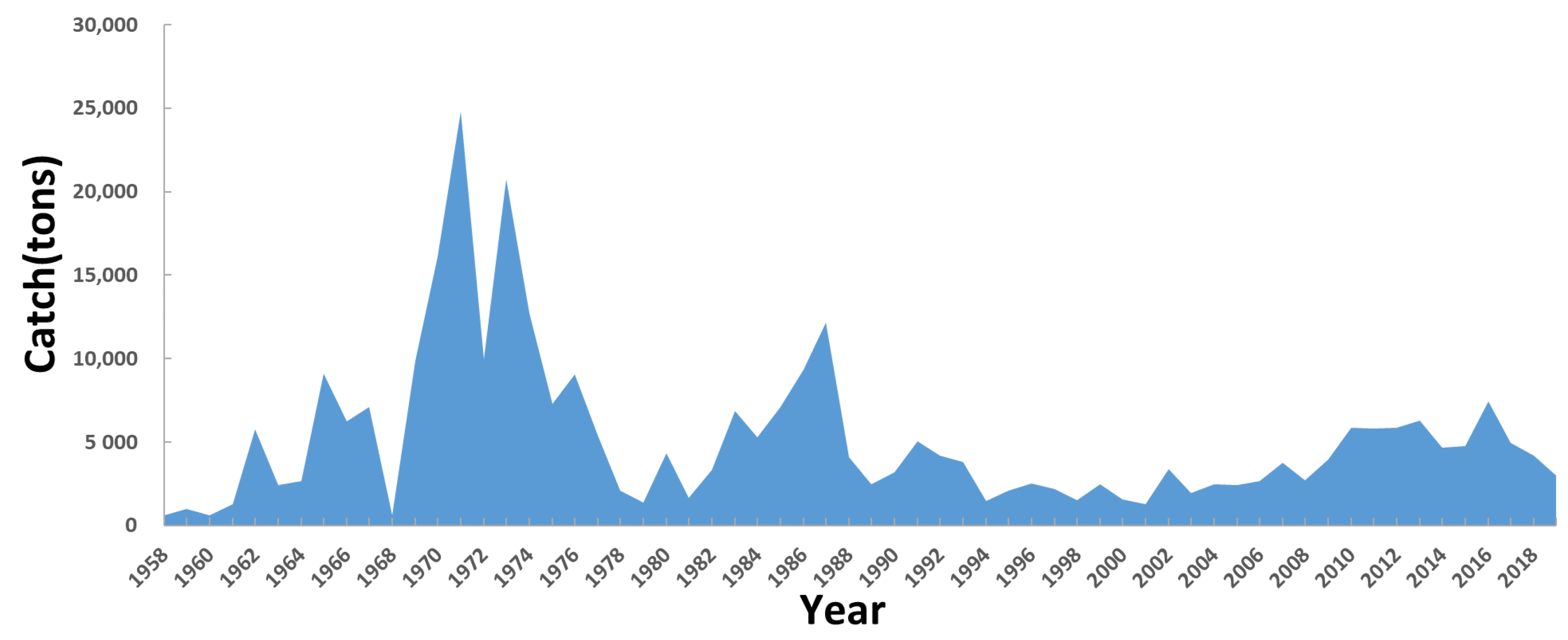
Figure 1. Estimated catch amount of sandfish from the East Sea from 1958 to 2019.
Sustainability 13 07868 g001
Figure 2. Estimated catch in weight of sandfish by fisheries in the East Sea from 2000 to 2019.
Sustainability 13 07868 g002
Figure 3. Trace plots of biomass (B), intrinsic growth (r), catchability coefficient (q), carrying capacity (K), and maximum sustainable yield (MSY).
Sustainability 13 07868 g003
Figure 4. Posterior densities of intrinsic growth (r), catchability coefficient (q), carrying capacity (K), maximum sustainable yield (MSY), biomass (2004), and biomass (2019).
Sustainability 13 07868 g004
Figure 5. Observed CPUE from the posterior predictive distribution of the CPUE.
Sustainability 13 07868 g005
Figure 6. Forecasting the biomass of sandfish by TAC- and fishing effort-based scenarios.
Sustainability 13 07868 g006
Table 1. Sandfish production by the Eastern Sea Danish fishery and its catch effort.
YearCatch (in MT)Horsepower (HP)
2004118316,914
200592317,142
2006102118,544
2007151418,656
2008187125,776
2009104216,557
2010125319,441
2011102716,659
2012164816,963
2013293616,588
2014203517,822
2015256917,011
2016405816,784
2017325517,360
2018238917,389
2019170517,796
Table 2. Standard and Monte Carlo errors of intrinsic growth (r), catchability coefficient (q), carrying capacity (K), maximum sustainable yield (MSY), and biomass.
ParameterBiomass (ton)
(2004)
Biomass (ton)
(2019)
Intrinsic
Growth
Catchability
Coefficient
Carrying
Capacity (ton)
MSY (ton)
Standard error240130880.14270.0000025298241319
Monte Carlo error891130.00160.0000001039532
MC
error/SE
3.6%3.6%1.1%3.8%4.0%2.4%
Table 3. Results of sandfish stock assessment models.
ParameterProcess-Error ModelState-Space Model
2.50%Median97.5%
MSY (ton)9820139130316500
BMSY (ton)34,316780014,19025,600
K68,63115,60028,38053,200
q0.000090.0000051210.0000084440.00001484
r0.380.200.420.76
0.570.99
RMSE3.0230.0029
Table 4. Results of the sandfish bioeconomic analysis.
TACStock
Biomass
(MT)
Catch
(MT)
NPV
(Thousand Won)
HPStock
Biomass
(MT)
Catch
(MT)
NPV
(Thousand Won)
Status Quo
(2019, Catch)
21,7711705241,776Status quo
(2019, HP)
17,8682685162,817
2196 MT
(2019, TAC)
18,8062196246,46260%12,590161157,964
50%7587329460,98050%13,273299279,233
30%13,3042855226,29430%15,0522940123,868
−30%22,5891537222,108−30%20,8152189164,140
−50%24,4461098172,599−50%26,3211978159,503
Publisher’s Note: MDPI stays neutral with regard to jurisdictional claims in published maps and institutional affiliations.