Power Distribution Network Expansion and Location Optimization of Additional Facilities: A Case Study

Abstract

Planning the power distribution network is critical and challenging; the main challenges include the multiple costs involved, selecting the appropriate locations of different nodes of the network at minimal cost, and minimizing the cost of energy loss for both the primary and secondary networks. Literature on the power distribution network presents different approaches, however, lacks to address the several issues of the complex power distribution networks and many aspects are yet to be explored; for example, the uncertain cost of energy loss. This study intends to address the gaps in the literature by proposing a four-phased approach. In doing so, first, an integer linear programming model is formulated with the objective of cost minimization. Secondly, fuzzy variables are used to tackle the parameters with uncertainty; cost of energy loss. In the third phase, a fine-tuned genetic algorithm (FT-GA) that uses the Taguchi Orthogonal Array is introduced to solve the mathematical model. It is worth mentioning that during the design of the experiment, the input parameters are crossover rate, elite count, and population size. In the last phase, a pragmatic approach is adopted and a Pakistan-based case study is used to validate the proposed model and its implication in real-life scenarios. The results exhibit that our proposed approach outperforms traditional methods like the genetic algorithm (GA) and inter-point methods in terms of fitness function value, number of generations, and computational time. This research contributes at both theoretical and managerial levels and may help decision-makers to design networks more efficiently and cost-effectively in Pakistan, Asia, and beyond.

1. Introduction

Electric power distribution system planning is far more challenging than the power generation itself mainly because of several factors; initial investment cost, maintenance cost, line losses, power losses, and consumer services. Previously, a few reasons behind the energy crisis in Pakistan have been the shortage of electricity, the increasing number of consumers, and fluctuating fuel prices. However, currently, the crisis is mainly due to a low voltage power supply and a poor distribution system. On the other hand, Pakistan needs to move toward renewable resources due to environmental concerns. This creates the need for new types of environmentally friendly power plants and a reengineered distribution networks within the country. In this regard, the government is planning to install renewable plants, including solar and wind plants, to accommodate the energy needs of the country. Designing the new distribution network with new facilities at minimum cost is a challenge. On one hand, the expansion of the existing power distribution network and inclusion of new power plants, new grid stations, substations in the primary network, and transformers in secondary networks will make the network more complex. Also, the redesign and execution of the new distribution network will have an immense cost. This requires a careful and efficient plan which focuses on high efficiency as well as the minimum cost at the same time. Furthermore, the connection of the main grids with the different number of substations at different locations and the connection with other facilities in the network would be a critical decision due to the huge investment cost of the transmission lines.

Due to previous experiences with poor transmission lines and the cost of maintenance, the government is also concerned about the power losses and the probability of faults occurring in transmission lines. Such a level of complex planning makes it a network optimization problem where there is a dire need to identify the exact size, cost, and location of new power plants, substations, grids, routes, and transmission line branches to connect various facilities in the network. The objective of the network planning is to reduce the overall investment cost of the new facilities, the maintenance cost of the lines and facilities in the network and reduce power losses with maximum customer satisfaction. 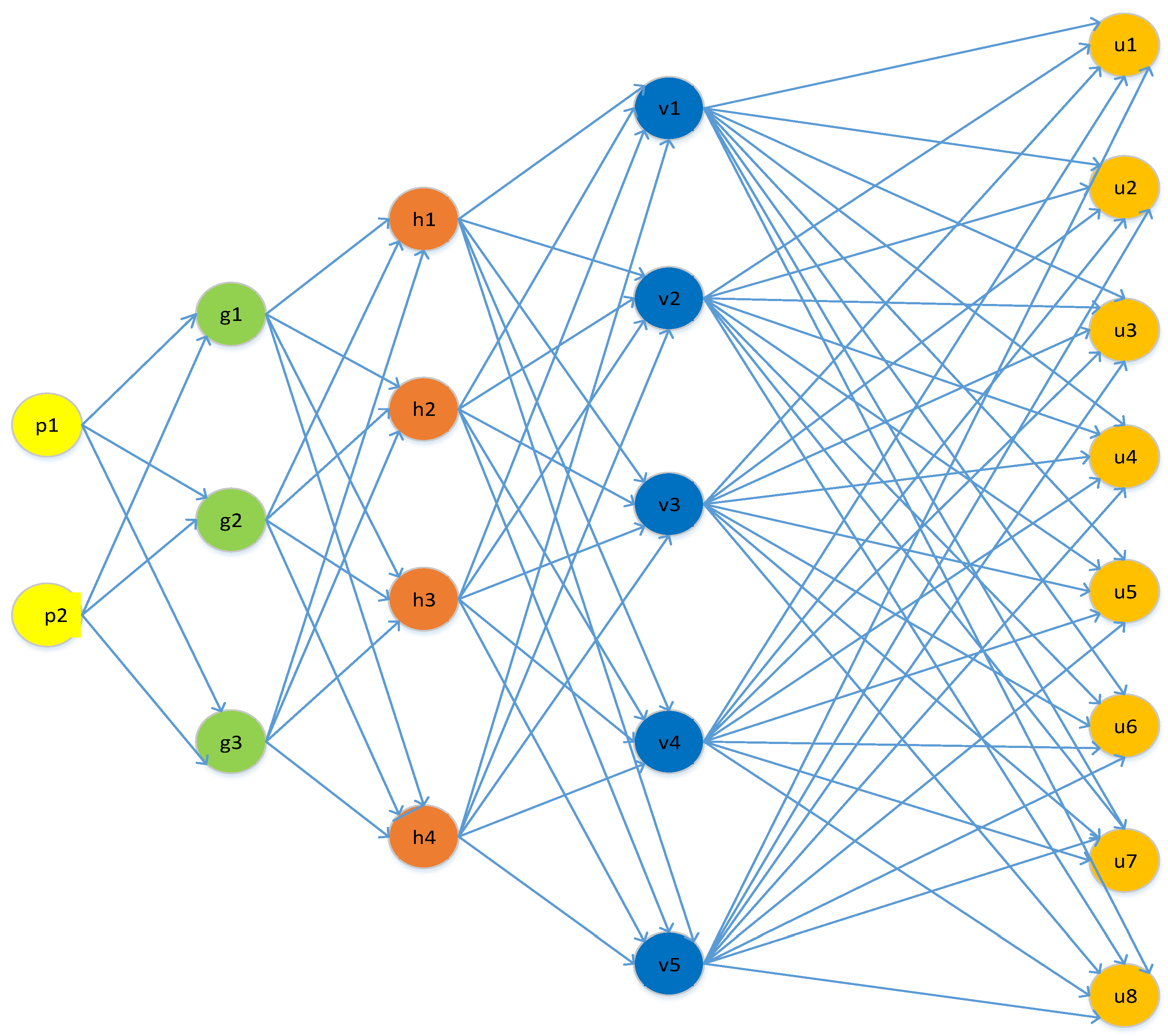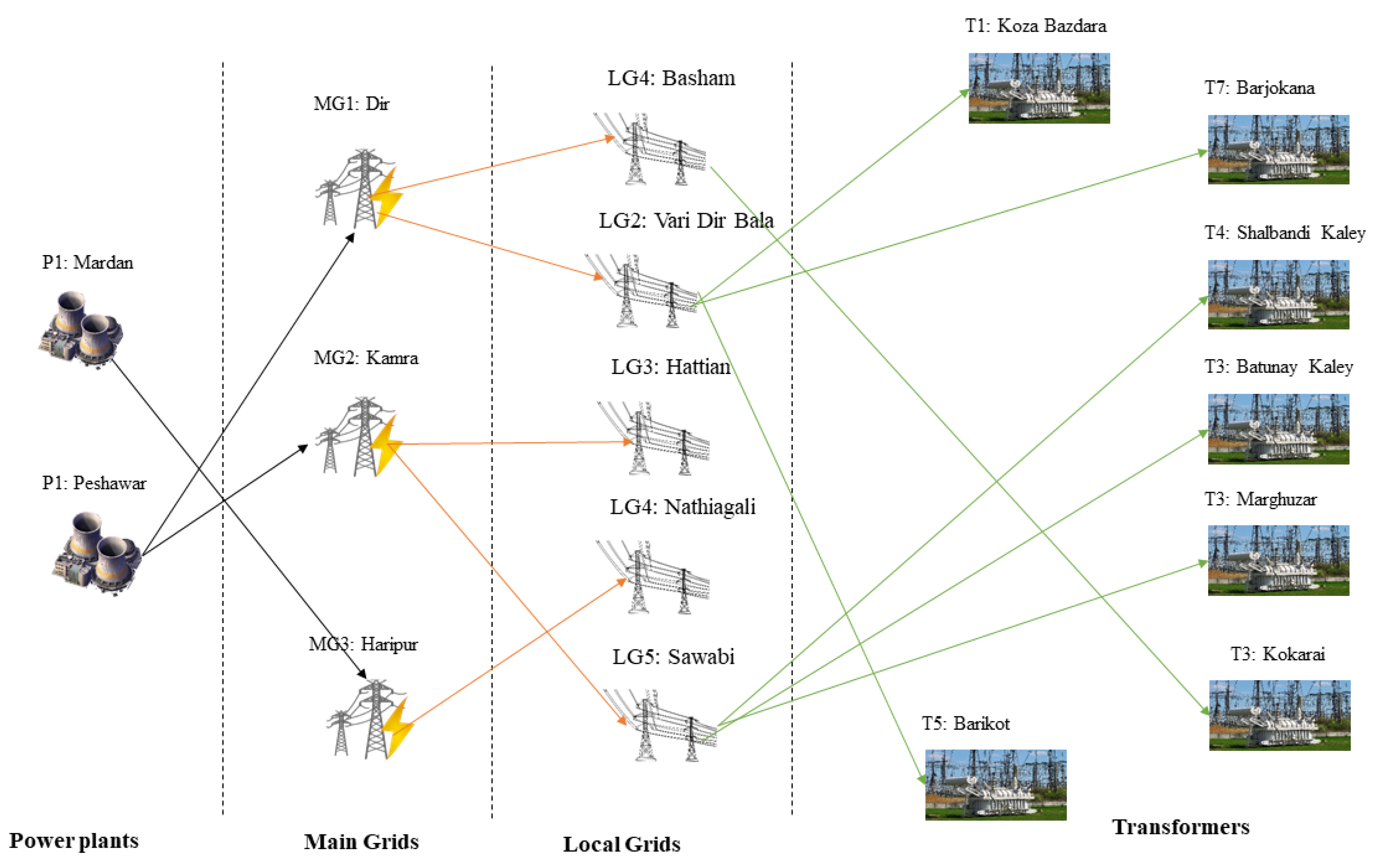For example, Figure 1 exhibits the complex nature of an electricity distribution supply chain network design that consists of power plants (p), main grids (g), local grids (h), and transformers (v), and customers (u). Power generation occurs at power plants, which are distributed to main grids, main grids distribute it to local grids, and finally, local grids are connected to transformers and users have connections with the transformers.

Based on the government’s concerns and the requirement of a new, expanded, and complex distribution network, this research proposes an optimization model that tends to select appropriate locations for plants, main grids, local grids, and transformers to reduce the total cost of installation and maintenance. Further, the model proposes that the decision to connect different power plants with main grids, main grids with local grids, and local grids with transformers is taken by minimizing the line losses as well as cost. This research focuses on the location-allocation of power plants, main grids, local grids, and transformers. In addition, it gives the optimal assignment of transformers to local grids, local grids to main grids, and main grids to the power plants. The objective includes minimizing the total cost, which is composed of fixed installation cost, maintenance cost, and energy costs, where energy cost is assumed to be uncertain during transmission and production. Our model addresses the shortcomings in the previously proposed models, for example, Gonela et al. [1] designed an electricity generation network considering production strategies without taking into account the line losses, decisions for location selection, and assignment of power plants and main grids. Similarly, Bayatloo [2] proposed a two-stage stochastic programming model for electricity supply chain network design by only considering location selection for power plants, main grids, and local grids to minimize the installation cost without considering the energy losses and maintenance in the supply chain network design. This model is an integration of the location-allocation and assignment model for the minimization of energy losses and maintenance cost that differentiate this model from previous literature Chen, Hsu, and Wu [3].

This study proposes a four-phase approach; in the first phase, a mixed-integer linear programming model is formulated that minimizes the total supply chain cost considering uncertain energy losses. In the second phase, the energy loss is regarded as a fuzzy variable in this research as the electricity supply chain networks are too complex and involve large-scale optimization. To optimize the supply chain network design in the third phase, a fine-tuned and hybridized genetic algorithm (GA) is introduced that can solve large optimization in reduced computation time and improved cost value. In the last step, a real case study of the electricity network is proposed. In addition, a set of numerical examples were also solved using other methods such as GA and interior point. Gap analysis is used to assess the solution quality of the proposed algorithm compared to the existing methods.

2. Literature Review

Electric power transmission is the mass transmission of electrical energy from its source—for example, a power plant—to an electrical substation where it is consumed [4]. The interconnected lines that carry this transmission are known as transmission lines [5]. However, electric power distribution and transmission lines have always been challenging because of their complex nature, the costs involved in their erection, and the cost of maintenance, and have been the focus of many researchers [6,7,8]. Mainly, literature on power distribution networks can be segregated into three dimensions; first, most of the researchers focused on the primary networks only [9,10,11,12,13,14,15,16], few focused on secondary [17], and only a few researchers addressed both the primary and secondary networks [18]. The second dimension is the selection of an objective function; for example, Paiva, Khodr, Dominguez-Navarro, Yusta, and Urdaneta [18] selected the investment cost and the cost of energy loss as the objective functions. Whereas Zhao, Wang, Yu, and Chen [15] considered optimal location and size of substations and feeders, and, Nahman and Peric [14] considered the optimal location of feeders in the network with the objective to minimize investment cost and cost of energy loss.

Similarly, Navarro and Rudnick [17] investigated the optimal location and size of substations and feeders with the objective to minimize the cost of investment as well as the cost of energy loss. Lavorato, Rider, Garcia, and Romero [12] and Lotero and Contreras [13] proposed a method to optimize the size and location of substations and feeders with the goal to minimize fixed and variable costs. Several other studies [9,10,11,13] considered the optimal location and size of substations, feeders, and distributed generation (DGs) to minimize the total cost. The literature shows that a lot of studies have been performed to address DGs for example, Ziari et al. [19] Studied the optimal location and size of substations, feeders, and DGs with the objective to minimize fixed and variable costs. In most of the studies, only the cost is considered as an optimization objective and few studies have taken reliability into consideration while identifying optimal distribution network expansion. Similarly, [20,21] focused on optimizing the size of substations and feeders with the objective to minimize the cost of investment, cost of energy loss with the constraints of voltage drops, which is concerned with reliability.

The installation year of DG in the distribution system has also been considered along with the optimal size and location of DG [22]. Another approach is presented by Gautam and Mithulananthan [23] who worked on optimal placement, including size, to formulate two different objectives, namely, social welfare maximization and profit maximization. Consumer payment, evaluated as a product of location marginal price (LMP) and load at each load bus, is proposed as another ranking to identify candidate nodes for DG placement. Optimal placement and size are identified for social welfare as well as profit maximization problems. Another study was carried out regarding DG in which Celli and Pilo [24] considered the optimal siting and sizing of DG units for a given network so that the cost of power losses during a prefixed period of study can be minimized and investments for grid upgrades can be deferred. The measures used in the literature for energy losses have the limitation that they do not take into consideration the future demand and robustness and flexibility of the network for future needs. The demand is variable and for the future demands of customers, the network is required to be reliable at handling uncertain power demands. For example, Ramírez-Rosado and Bernal-Agustín [25] considered the optimal expansion of an existing distribution system, to meet its forecasted future power demands, determining the optimal sizing and location of future feeders (reserve feeders and operation feeders) and substations, and the optimal feeder reinforcements and/or substitution of the existing feeders, as well as the optimal size increase of the existing substations, with an objective function to reduce economic cost.

The third dimension of the literature reflects the methodology used for optimizing in general and network design in particular. For example, AlRashidi and AlHajri [26] presented an improved particle swarm optimization algorithm (PSO) for the optimal planning of multiple DGs sources. Some studies used Pareto optimization concepts [27,28,29,30], especially, Carrano, Soares, Takahashi, Saldanha, and Neto [27] presented a multi-objective approach to optimizing electric distribution networks using a multi-objective genetic algorithm (MO-GA) to get a Pareto solution for their proposed problem. Further, Mendoza, Bernal-Agustin, and Domínguez-Navarro [29] used the Non-Dominated Sorting Genetic Algorithm (NSGA) and Strength Pareto Evolutionary Algorithm (SPEA) for multi-objective optimization and also proposed a fuzzy c-mean clustering algorithm for their considered problem. Moreover, Soroudi and Ehsan [30] considered a multi-objective model for the distribution generation investment with the aim to optimize active losses, costs, and environmental emissions simultaneously to determine the optimal scheme of sizing and sitting of DGs. They obtained Pareto solutions using GA and a fuzzy satisfying method. Also, Cossi, Da Silva, Lazaro, and Mantovani [28] formulated and presented a multi-objective simulated annealing algorithm to solve and get the Pareto results of the proposed problem. On the other hand, Khalesi et al. [31] considered a multi-objective model for DGs to determine the optimal locations to place DGs in the distribution system with the aim to minimize power loss of the system and enhance reliability improvement and voltage profile.

García and Mena [32] used a new evolutionary method called Teaching–Learning Based Optimization (TLBO) algorithm to find the best sites to connect DG systems in a distribution network, choosing among a large number of potential combinations to determine the optimal placement and size of Distributed Generation (DG) units in distribution systems. Fan and Jen [33] introduced enhanced partial search approaches in the particle swarm algorithm to solve optimization problems in the supply chain. Furthermore, most of the literature focused on the existing power distribution models developed is focused on the conventional power generators including diesel units and turbines [34]. However, due to environmental concerns and the shortage of conventional power plants, there is a need to develop models that can consider both types of power generators including conventional and renewable energy power generators, that is, solar power plants and wind turbines. Researchers like Gupta et al. [35] discussed the integration of DGs into the present supply chain and Khatod et al. [36] contributed to handling the uncertainties associated with load and renewable resources (wind and solar) to overcome issues in the continuous supply of power and discussed the optimal placement of photovoltaic arrays (PVAs) and wind turbine generators WTGs in a radial distribution system. Further, Mena et al. [37] proposed a framework for the optimal size and location of the distributed renewable generation units (DG) and also considered the uncertainties in renewable resources availability, components failure and repair events, load and grid power supply. They aimed at simultaneous minimization of the energy not supplied and global cost. Atwa et al. [38] presented a technique for the optimal allocation of different types of renewable distributed generation (DG) units, that is, wind-based DG, solar DG, and biomass DG in the distribution system with the aim to minimize annual energy loss. The global dependence on fossil fuels is dangerous to our environment in terms of their emissions unless specific policies and measures are put in place [39]. Nevertheless, their research reveals that a reduction in the emissions of these gases is possible with the widespread adoption of distributed generation (DG) technologies that feed on renewable energy sources, in the generation of electric power. The main objective of their work is to reduce the harmful effect of the emission of greenhouse gases thus reducing the public concerns over human health risks caused by the conventional method of electricity generation.

In the literature, very little work has been carried out on allocation and assignment simultaneously. For example, García and Mena, Hosseini and Jenab [40] worked on the expansion policy of power plant centers involving the choice of regions that must be allocated to power plant centers and power plant centers capacities over a specified planning horizon (years) were tackled. Nevertheless, in most of the studies, a single objective has been considered for the design of the optimal network. However, in real cases, more than one objective is desired to optimize the network design problems. Fan et al. [41] proposed an algorithm that used the concept of Pareto dominance in multi-objective particle swarm algorithm with empirical-movement diversified-search. Most of the electricity distribution problems are nonlinear in nature and require special metaheuristics. However, the use of metaheuristics requires the management of parameters used in computations. Zahara and Fan [42] introduced a real code genetic algorithm to solve stochastic optimization problems such as energy losses in electricity distribution networks.

In the literature, most of the studies have considered expansion planning in the primary network in terms of multi-objective optimization [17,18,19,20]. However, primary and secondary grids are both important in the distribution network expansion and planning to get a global solution. A few research studies have investigated the planning of primary and secondary networks together [18,20,21]. However, they added the costs of primary and secondary grids to make a single objective optimization problem.

A few other studies in the literature [16,19,43,44,45] considered both primary and secondary networks simultaneously. However, they also optimize the network with the single objective being minimizing the fixed and variable costs. The current research addresses an optimization model for the electricity distribution network. In the electricity distribution network, facilities such as power plants, main grids, local grids are connected with the help of transmission lines. The main objective of the research is to minimize the total cost of installation of new facilities, maintenance cost, and energy loss cost. Energy loss is the function of distance and temperature, so it is considered uncertain in this model. The uncertainty is modeled using fuzzy variables. To solve this integer linear programming issue, a fine-tuned genetic algorithm is used. The fine-tuning is carried out using the Taguchi design of experiments. The consideration of uncertain energy loss in the cost function and the use of Taguchi-based fine-tuned GA differentiate this research from the previous literature.

3. Development of Mathematical Model

The objective function is formulated based on the assumptions below and Notation presented in Table 1.

3.1. Problem Statement

Electric power distribution systems are very complex in nature as these may include hundreds of thousands of components: generators, grids, transformers, transmission lines, and customers, etc. The current energy crisis in Pakistan has increased the need for efficient planning and expansion of the power distribution network in the country.

3.2. Model Assumptions

The proposed model is based on the following assumptions:

• The capacity of each power plant, main grid, local grid, and transformer is not the same and is known.
• The maintenance and installation costs of power plants, main grid, local grids, transformers, and transmission lines are known.
• The energy loss cost is assumed to be uncertain and is treated as a fuzzy variable.

3.3. Model Notation and Abbreviations

See Table 1.

Table 1. Nomenclature table.

Sets
$p$	$\mathrm{power} \mathrm{plants} p=1,2,3,\dots ,P$
$g$	$\mathrm{main} \mathrm{grids} g=1,2,3,\dots ,G$
$h$	$\mathrm{local} \mathrm{grids} h=1,2,3,\dots ,H$
$v$	$\mathrm{transformers} v=1,2,3,\dots ,V$
$l^p$	$\mathrm{location} \mathrm{of} \mathrm{power} \mathrm{plant} “p”$$l^p=1,2,3,\dots ,L^P$
$l^g$	$\mathrm{location} \mathrm{of} \mathrm{main} \mathrm{grid} “g”$$l^g=1,2,3,\dots ,L^G$
$l^h$	$\mathrm{location} \mathrm{of} \mathrm{local} \mathrm{grid} “h”$$l^h=1,2,3,\dots ,L^H$
$l^v$	$\mathrm{location} \mathrm{of} \mathrm{transformer} “v”$$l^v=1,2,3,\dots ,L^V$
Parameters
$F{C}_p^{l^p}$	$\mathrm{fixed} \cos \mathrm{t} \mathrm{of} \mathrm{installation} \mathrm{power} \mathrm{plant} “p”$$\mathrm{at} \mathrm{location} “l^p”$
$M{C}_g^{{\mathrm{l}}^g}$	$\mathrm{maintenance} \cos \mathrm{t} \mathrm{of} \mathrm{main} \mathrm{grid} “g”$$\mathrm{at} \mathrm{location} “l^g”$
$F{C}_g^{l^g}$	$\mathrm{fixed} \cos \mathrm{t} \mathrm{of} \mathrm{main} \mathrm{grid} “g”$$\mathrm{at} \mathrm{location} “l^g”$
$M{C}_h^{l^h}$	$\mathrm{maintenance} \cos \mathrm{t} \mathrm{of} \mathrm{local} \mathrm{grid} “h”$$\mathrm{at} \mathrm{location} “l^h”$
$F{C}_h^{l^h}$	$\mathrm{fixed} \cos \mathrm{t} \mathrm{of} \mathrm{local} \mathrm{grid} “h”$$\mathrm{at} \mathrm{location} “l^h”$
$M{C}_v^{l^v}$	$\mathrm{maintenance} \cos \mathrm{t} \mathrm{of} \mathrm{transformer} “v”$$\mathrm{at} \mathrm{location} “l^v”$
$M{C}_{pg}^{l^p{l}^g}$	$\mathrm{maintenance} \cos \mathrm{t} \mathrm{of} \mathrm{transmission} \mathrm{line} \mathrm{between} \mathrm{plant} “p”$$\mathrm{at} \mathrm{location} “l^p”$$\mathrm{and} \mathrm{main} \mathrm{grid} “g”$$\mathrm{at} \mathrm{location} “l^g”$
$F{C}_{pg}^{l^p{l}^g}$	$\mathrm{fixed} \cos \mathrm{t} \mathrm{of} \mathrm{installation} \mathrm{of} \mathrm{transmission} \mathrm{line} \mathrm{between} “p”$$\mathrm{at} \mathrm{location} “l^p”$$\mathrm{and} \mathrm{main} \mathrm{grid} “g”$$\mathrm{at} \mathrm{location} “l^g”$
$M{C}_{gh}^{l^g{l}^h}$	$\mathrm{maintenance} \cos \mathrm{t} \mathrm{of} \mathrm{transmission} \mathrm{line} \mathrm{between} \mathrm{main} \mathrm{grid} “g”$$\mathrm{at} \mathrm{location} “l^g”$$\mathrm{and} \mathrm{local} \mathrm{grid} “h”$$\mathrm{at} \mathrm{location} “l^h”$
$F{C}_{gh}^{l^g{l}^h}$	$\mathrm{fixed} \cos \mathrm{t} \mathrm{of} \mathrm{installation} \mathrm{of} \mathrm{transmission} \mathrm{line} \mathrm{between} \mathrm{main} \mathrm{grid} “g”$$\mathrm{at} \mathrm{location} “l^g”$$\mathrm{and} \mathrm{local} \mathrm{grid} “h”$$\mathrm{at} \mathrm{location} “l^h”$
$M{C}_{hv}^{l^h{l}^v}$	$\mathrm{maintenance} \cos \mathrm{t} \mathrm{of} \mathrm{transmission} \mathrm{line} \mathrm{between} \mathrm{local} \mathrm{grid} “h”$$\mathrm{at} \mathrm{location} “l^h”$$\mathrm{and} \mathrm{transformer}“v”$$\mathrm{at} \mathrm{location} “l^v”$
$F{C}_{hv}^{l^h{l}^v}$	$\mathrm{fixed} \cos \mathrm{t} \mathrm{of} \mathrm{installation} \mathrm{of} \mathrm{transmission} \mathrm{line} \mathrm{between} \mathrm{local} \mathrm{grid} “h”$$\mathrm{at} \mathrm{location} “l^h”$$\mathrm{and} \mathrm{transformer} “v”$$\mathrm{at} \mathrm{location} “l^v”$
$M{C}_{vu}^{l^v{l}^u}$	$\mathrm{maintenance} \cos \mathrm{t} \mathrm{of} \mathrm{transmission} \mathrm{line} \mathrm{between} \mathrm{transformer} “v”$$\mathrm{at} \mathrm{location} “l^v”$$\mathrm{and} \mathrm{users} “u”$ at location “lu”
$F{C}_{uv}^{l^v{l}^u}$	$\mathrm{fixed} \cos \mathrm{t} \mathrm{of} \mathrm{installation} \mathrm{of} \mathrm{transmission} \mathrm{line} \mathrm{between} \mathrm{transformer} “v”$$\mathrm{at} \mathrm{location} “l^v”$$\mathrm{and} \mathrm{users} “u”$$\mathrm{at} \mathrm{location} “l^u”$
$EL{C}_{pg}^{l^p{l}^g}$	$\mathrm{energy} \mathrm{loss} \cos \mathrm{t} \mathrm{of} \mathrm{transmission} \mathrm{lines} \mathrm{from} \mathrm{power} \mathrm{plant} “p”$$\mathrm{at} \mathrm{location} “l^p”$$\mathrm{to} \mathrm{main} \mathrm{grid} “g”$$\mathrm{at} \mathrm{location} “l^g”$
$EL{C}_{gh}^{l^g{l}^h}$	$\mathrm{energy} \mathrm{loss} \cos \mathrm{t} \mathrm{of} \mathrm{transmission} \mathrm{lines} \mathrm{from} \mathrm{main} \mathrm{grid} “g”$$\mathrm{at} \mathrm{location} “l^g”$$\mathrm{to} \mathrm{local} \mathrm{grid} “h”$$\mathrm{at} \mathrm{location} “l^h”$
$EL{C}_{hv}^{l^h{l}^v}$	$\mathrm{energy} \mathrm{loss} \cos \mathrm{t} \mathrm{of} \mathrm{transmission} \mathrm{lines} \mathrm{from} \mathrm{local} \mathrm{grid} “h”$$\mathrm{at} \mathrm{location} “l^h”$$\mathrm{to} \mathrm{transformer}“v”$$\mathrm{at} \mathrm{location} “l^v”$
$EL{C}_{vu}^{l^v{l}^u}$	$\mathrm{energy} \mathrm{loss} \cos \mathrm{t} \mathrm{of} \mathrm{transmission} \mathrm{lines} \mathrm{from} \mathrm{transformer} “v”$$\mathrm{at} \mathrm{location} “l^v”$$\mathrm{to} \mathrm{users} “u”$$\mathrm{at} \mathrm{location} “l^u”$
Decision Variables
$y_p^{l^p}=\left\{\begin{array}{cc}1& \mathrm{if}\hspace{0.17em}\mathrm{power}\hspace{0.17em}\mathrm{plant}\hspace{0.17em}“p”\hspace{0.17em}\mathrm{is}\hspace{0.17em}\mathrm{installed}\hspace{0.17em}\mathrm{at}\hspace{0.17em}\mathrm{location}“l^{p_{}}”\\ 0& \mathrm{otherwise}\end{array}\right\}$ $y_g^{l^g}=\left\{\begin{array}{cc}1& \mathrm{if}\hspace{0.17em}\mathrm{grid}\hspace{0.17em}“g”\hspace{0.17em}\mathrm{is}\hspace{0.17em}\mathrm{installed}\hspace{0.17em}\mathrm{at}\hspace{0.17em}\mathrm{location}“l^g”\\ 0& \mathrm{otherwise}\end{array}\right\}$ $y_h^{l^h}=\left\{\begin{array}{cc}1& \begin{array}{l}\mathrm{if}\hspace{0.17em}\mathrm{local}\hspace{0.17em}\mathrm{grid}\hspace{0.17em}“h”\hspace{0.17em}\mathrm{is}\hspace{0.17em}\mathrm{installed}\hspace{0.17em}\mathrm{at}\hspace{0.17em}\mathrm{location}“l^h”\\ \end{array}\\ 0& \mathrm{otherwise}\end{array}\right\}$ $y_v^{l^v}=\left\{\begin{array}{cc}1& \mathrm{if}\hspace{0.17em}\mathrm{transformer}\hspace{0.17em}“v”\hspace{0.17em}\mathrm{is}\hspace{0.17em}\mathrm{installed}\hspace{0.17em}\mathrm{at}\hspace{0.17em}\mathrm{location}“l^v”\\ 0& \mathrm{otherwise}\end{array}\right\}$ $z_{pg}^{l^g{l}^p}=\left\{\begin{array}{cc}1& \mathrm{if}\hspace{0.17em}\mathrm{main}\hspace{0.17em}\mathrm{grid}\hspace{0.17em}“g”\hspace{0.17em}\mathrm{at}\hspace{0.17em}\mathrm{location}\hspace{0.17em}“l^g”\hspace{0.17em}\mathrm{is}\hspace{0.17em}\mathrm{connected}\hspace{0.17em}\mathrm{to}\hspace{0.17em}\mathrm{the}\hspace{0.17em}\mathrm{power}\hspace{0.17em}\mathrm{plant}\hspace{0.17em}“p”\hspace{0.17em}\mathrm{at}\hspace{0.17em}\mathrm{location}\hspace{0.17em}“l^p”\\ 0& \mathrm{otherwise}\end{array}\right\}$ $z_{gh}^{l^h{l}^g}=\left\{\begin{array}{cc}1& \mathrm{if}\hspace{0.17em}\mathrm{local}\hspace{0.17em}\mathrm{grid}\hspace{0.17em}“h”\hspace{0.17em}\mathrm{at}\hspace{0.17em}\mathrm{location}\hspace{0.17em}“l^h”\hspace{0.17em}\mathrm{is}\hspace{0.17em}\mathrm{connected}\hspace{0.17em}\mathrm{to}\hspace{0.17em}\mathrm{the}\hspace{0.17em}\mathrm{main}\hspace{0.17em}\mathrm{grid}\hspace{0.17em}“g”\hspace{0.17em}\mathrm{at}\hspace{0.17em}\mathrm{location}\hspace{0.17em}“l^g”\\ 0& \mathrm{otherwise}\end{array}\right\}$ $z_{hv}^{l^v{l}^h}=\left\{\begin{array}{cc}1& \mathrm{if}\hspace{0.17em}\mathrm{transformer}\hspace{0.17em}“v”\hspace{0.17em}\mathrm{at}\hspace{0.17em}\mathrm{location}\hspace{0.17em}“l^v”\mathrm{is}\hspace{0.17em}\mathrm{connected}\hspace{0.17em}\mathrm{to}\hspace{0.17em}\mathrm{the}\hspace{0.17em}\mathrm{local}\hspace{0.17em}\mathrm{grid}\hspace{0.17em}“h”\hspace{0.17em}\mathrm{at}\hspace{0.17em}\mathrm{location}\hspace{0.17em}“l^h”\\ 0& \mathrm{otherwise}\end{array}\right\}$

Table 1. Nomenclature table.

Sets
$p$	$\mathrm{power} \mathrm{plants} p=1,2,3,\dots ,P$
$g$	$\mathrm{main} \mathrm{grids} g=1,2,3,\dots ,G$
$h$	$\mathrm{local} \mathrm{grids} h=1,2,3,\dots ,H$
$v$	$\mathrm{transformers} v=1,2,3,\dots ,V$
$l^p$	$\mathrm{location} \mathrm{of} \mathrm{power} \mathrm{plant} “p”$$l^p=1,2,3,\dots ,L^P$
$l^g$	$\mathrm{location} \mathrm{of} \mathrm{main} \mathrm{grid} “g”$$l^g=1,2,3,\dots ,L^G$
$l^h$	$\mathrm{location} \mathrm{of} \mathrm{local} \mathrm{grid} “h”$$l^h=1,2,3,\dots ,L^H$
$l^v$	$\mathrm{location} \mathrm{of} \mathrm{transformer} “v”$$l^v=1,2,3,\dots ,L^V$
Parameters
$F{C}_p^{l^p}$	$\mathrm{fixed} \cos \mathrm{t} \mathrm{of} \mathrm{installation} \mathrm{power} \mathrm{plant} “p”$$\mathrm{at} \mathrm{location} “l^p”$
$M{C}_g^{{\mathrm{l}}^g}$	$\mathrm{maintenance} \cos \mathrm{t} \mathrm{of} \mathrm{main} \mathrm{grid} “g”$$\mathrm{at} \mathrm{location} “l^g”$
$F{C}_g^{l^g}$	$\mathrm{fixed} \cos \mathrm{t} \mathrm{of} \mathrm{main} \mathrm{grid} “g”$$\mathrm{at} \mathrm{location} “l^g”$
$M{C}_h^{l^h}$	$\mathrm{maintenance} \cos \mathrm{t} \mathrm{of} \mathrm{local} \mathrm{grid} “h”$$\mathrm{at} \mathrm{location} “l^h”$
$F{C}_h^{l^h}$	$\mathrm{fixed} \cos \mathrm{t} \mathrm{of} \mathrm{local} \mathrm{grid} “h”$$\mathrm{at} \mathrm{location} “l^h”$
$M{C}_v^{l^v}$	$\mathrm{maintenance} \cos \mathrm{t} \mathrm{of} \mathrm{transformer} “v”$$\mathrm{at} \mathrm{location} “l^v”$
$M{C}_{pg}^{l^p{l}^g}$	$\mathrm{maintenance} \cos \mathrm{t} \mathrm{of} \mathrm{transmission} \mathrm{line} \mathrm{between} \mathrm{plant} “p”$$\mathrm{at} \mathrm{location} “l^p”$$\mathrm{and} \mathrm{main} \mathrm{grid} “g”$$\mathrm{at} \mathrm{location} “l^g”$
$F{C}_{pg}^{l^p{l}^g}$	$\mathrm{fixed} \cos \mathrm{t} \mathrm{of} \mathrm{installation} \mathrm{of} \mathrm{transmission} \mathrm{line} \mathrm{between} “p”$$\mathrm{at} \mathrm{location} “l^p”$$\mathrm{and} \mathrm{main} \mathrm{grid} “g”$$\mathrm{at} \mathrm{location} “l^g”$
$M{C}_{gh}^{l^g{l}^h}$	$\mathrm{maintenance} \cos \mathrm{t} \mathrm{of} \mathrm{transmission} \mathrm{line} \mathrm{between} \mathrm{main} \mathrm{grid} “g”$$\mathrm{at} \mathrm{location} “l^g”$$\mathrm{and} \mathrm{local} \mathrm{grid} “h”$$\mathrm{at} \mathrm{location} “l^h”$
$F{C}_{gh}^{l^g{l}^h}$	$\mathrm{fixed} \cos \mathrm{t} \mathrm{of} \mathrm{installation} \mathrm{of} \mathrm{transmission} \mathrm{line} \mathrm{between} \mathrm{main} \mathrm{grid} “g”$$\mathrm{at} \mathrm{location} “l^g”$$\mathrm{and} \mathrm{local} \mathrm{grid} “h”$$\mathrm{at} \mathrm{location} “l^h”$
$M{C}_{hv}^{l^h{l}^v}$	$\mathrm{maintenance} \cos \mathrm{t} \mathrm{of} \mathrm{transmission} \mathrm{line} \mathrm{between} \mathrm{local} \mathrm{grid} “h”$$\mathrm{at} \mathrm{location} “l^h”$$\mathrm{and} \mathrm{transformer}“v”$$\mathrm{at} \mathrm{location} “l^v”$
$F{C}_{hv}^{l^h{l}^v}$	$\mathrm{fixed} \cos \mathrm{t} \mathrm{of} \mathrm{installation} \mathrm{of} \mathrm{transmission} \mathrm{line} \mathrm{between} \mathrm{local} \mathrm{grid} “h”$$\mathrm{at} \mathrm{location} “l^h”$$\mathrm{and} \mathrm{transformer} “v”$$\mathrm{at} \mathrm{location} “l^v”$
$M{C}_{vu}^{l^v{l}^u}$	$\mathrm{maintenance} \cos \mathrm{t} \mathrm{of} \mathrm{transmission} \mathrm{line} \mathrm{between} \mathrm{transformer} “v”$$\mathrm{at} \mathrm{location} “l^v”$$\mathrm{and} \mathrm{users} “u”$ at location “lu”
$F{C}_{uv}^{l^v{l}^u}$	$\mathrm{fixed} \cos \mathrm{t} \mathrm{of} \mathrm{installation} \mathrm{of} \mathrm{transmission} \mathrm{line} \mathrm{between} \mathrm{transformer} “v”$$\mathrm{at} \mathrm{location} “l^v”$$\mathrm{and} \mathrm{users} “u”$$\mathrm{at} \mathrm{location} “l^u”$
$EL{C}_{pg}^{l^p{l}^g}$	$\mathrm{energy} \mathrm{loss} \cos \mathrm{t} \mathrm{of} \mathrm{transmission} \mathrm{lines} \mathrm{from} \mathrm{power} \mathrm{plant} “p”$$\mathrm{at} \mathrm{location} “l^p”$$\mathrm{to} \mathrm{main} \mathrm{grid} “g”$$\mathrm{at} \mathrm{location} “l^g”$
$EL{C}_{gh}^{l^g{l}^h}$	$\mathrm{energy} \mathrm{loss} \cos \mathrm{t} \mathrm{of} \mathrm{transmission} \mathrm{lines} \mathrm{from} \mathrm{main} \mathrm{grid} “g”$$\mathrm{at} \mathrm{location} “l^g”$$\mathrm{to} \mathrm{local} \mathrm{grid} “h”$$\mathrm{at} \mathrm{location} “l^h”$
$EL{C}_{hv}^{l^h{l}^v}$	$\mathrm{energy} \mathrm{loss} \cos \mathrm{t} \mathrm{of} \mathrm{transmission} \mathrm{lines} \mathrm{from} \mathrm{local} \mathrm{grid} “h”$$\mathrm{at} \mathrm{location} “l^h”$$\mathrm{to} \mathrm{transformer}“v”$$\mathrm{at} \mathrm{location} “l^v”$
$EL{C}_{vu}^{l^v{l}^u}$	$\mathrm{energy} \mathrm{loss} \cos \mathrm{t} \mathrm{of} \mathrm{transmission} \mathrm{lines} \mathrm{from} \mathrm{transformer} “v”$$\mathrm{at} \mathrm{location} “l^v”$$\mathrm{to} \mathrm{users} “u”$$\mathrm{at} \mathrm{location} “l^u”$
Decision Variables
$y_p^{l^p}=\left\{\begin{array}{cc}1& \mathrm{if}\hspace{0.17em}\mathrm{power}\hspace{0.17em}\mathrm{plant}\hspace{0.17em}“p”\hspace{0.17em}\mathrm{is}\hspace{0.17em}\mathrm{installed}\hspace{0.17em}\mathrm{at}\hspace{0.17em}\mathrm{location}“l^{p_{}}”\\ 0& \mathrm{otherwise}\end{array}\right\}$ $y_g^{l^g}=\left\{\begin{array}{cc}1& \mathrm{if}\hspace{0.17em}\mathrm{grid}\hspace{0.17em}“g”\hspace{0.17em}\mathrm{is}\hspace{0.17em}\mathrm{installed}\hspace{0.17em}\mathrm{at}\hspace{0.17em}\mathrm{location}“l^g”\\ 0& \mathrm{otherwise}\end{array}\right\}$ $y_h^{l^h}=\left\{\begin{array}{cc}1& \begin{array}{l}\mathrm{if}\hspace{0.17em}\mathrm{local}\hspace{0.17em}\mathrm{grid}\hspace{0.17em}“h”\hspace{0.17em}\mathrm{is}\hspace{0.17em}\mathrm{installed}\hspace{0.17em}\mathrm{at}\hspace{0.17em}\mathrm{location}“l^h”\\ \end{array}\\ 0& \mathrm{otherwise}\end{array}\right\}$ $y_v^{l^v}=\left\{\begin{array}{cc}1& \mathrm{if}\hspace{0.17em}\mathrm{transformer}\hspace{0.17em}“v”\hspace{0.17em}\mathrm{is}\hspace{0.17em}\mathrm{installed}\hspace{0.17em}\mathrm{at}\hspace{0.17em}\mathrm{location}“l^v”\\ 0& \mathrm{otherwise}\end{array}\right\}$ $z_{pg}^{l^g{l}^p}=\left\{\begin{array}{cc}1& \mathrm{if}\hspace{0.17em}\mathrm{main}\hspace{0.17em}\mathrm{grid}\hspace{0.17em}“g”\hspace{0.17em}\mathrm{at}\hspace{0.17em}\mathrm{location}\hspace{0.17em}“l^g”\hspace{0.17em}\mathrm{is}\hspace{0.17em}\mathrm{connected}\hspace{0.17em}\mathrm{to}\hspace{0.17em}\mathrm{the}\hspace{0.17em}\mathrm{power}\hspace{0.17em}\mathrm{plant}\hspace{0.17em}“p”\hspace{0.17em}\mathrm{at}\hspace{0.17em}\mathrm{location}\hspace{0.17em}“l^p”\\ 0& \mathrm{otherwise}\end{array}\right\}$ $z_{gh}^{l^h{l}^g}=\left\{\begin{array}{cc}1& \mathrm{if}\hspace{0.17em}\mathrm{local}\hspace{0.17em}\mathrm{grid}\hspace{0.17em}“h”\hspace{0.17em}\mathrm{at}\hspace{0.17em}\mathrm{location}\hspace{0.17em}“l^h”\hspace{0.17em}\mathrm{is}\hspace{0.17em}\mathrm{connected}\hspace{0.17em}\mathrm{to}\hspace{0.17em}\mathrm{the}\hspace{0.17em}\mathrm{main}\hspace{0.17em}\mathrm{grid}\hspace{0.17em}“g”\hspace{0.17em}\mathrm{at}\hspace{0.17em}\mathrm{location}\hspace{0.17em}“l^g”\\ 0& \mathrm{otherwise}\end{array}\right\}$ $z_{hv}^{l^v{l}^h}=\left\{\begin{array}{cc}1& \mathrm{if}\hspace{0.17em}\mathrm{transformer}\hspace{0.17em}“v”\hspace{0.17em}\mathrm{at}\hspace{0.17em}\mathrm{location}\hspace{0.17em}“l^v”\mathrm{is}\hspace{0.17em}\mathrm{connected}\hspace{0.17em}\mathrm{to}\hspace{0.17em}\mathrm{the}\hspace{0.17em}\mathrm{local}\hspace{0.17em}\mathrm{grid}\hspace{0.17em}“h”\hspace{0.17em}\mathrm{at}\hspace{0.17em}\mathrm{location}\hspace{0.17em}“l^h”\\ 0& \mathrm{otherwise}\end{array}\right\}$

3.4. Formulation of Objective Function and Constraints

Equation (1) is the total cost function in which the first four terms show the maintenance and fixed installation cost, the last three terms indicate maintenance and energy loss cost of transmission lines. It is an integer linear programming model because all decision variables are binary in nature. As a novel approach, the cost of energy loss was considered to be uncertain in the objective function of the model. To model the uncertainty, the cost of energy loss was treated as a fuzzy variable assuming that it follows a trapezoidal membership function. In order to make a variable fuzzy, the crisp input is converted to the fuzzy number [46,47,48,49]. Then fuzzy numbers are evaluated using logical rules. Figure 2 describes the fuzzy inference process.

$$\begin{array}{l}Minimize\hspace{0.17em}\hspace{0.17em}\hspace{0.17em}TC={\displaystyle \sum _{p,l^p=1}^{P,L^p}(M{C}_p^{l^p}+F{C}_p^{l^p})\times y_p^{l^p}}+{\displaystyle \sum _{g,l^g=1}^{G,L^G}(M{C}_g^{l^g}+F{C}_g^{l^g})\times y_g^{l^g}}\\ +{\displaystyle \sum _{h,l^h=1}^{H,L^H}(M{C}_h^{l^h}+F{C}_h^{l^h})\times y_h^{l^h}}+{\displaystyle \sum _{v,l^v=1}^{V,L^V}(M{C}_v^{l^v}+F{C}_v^{l^v})\times y_v^{l^v}}+\\ {\displaystyle \sum _{pg,l^{pg}=1}^{PG,L^p{L}^G}(M{C}_{pg}^{l^p{l}^g}+\widetilde{EL{C}_{pg}^{l^p{l}^g}})\times z_{pg}^{l^p{l}^g}}+{\displaystyle \sum _{gh,l^{gh}=1}^{GH,L^G{L}^H}(M{C}_{gh}^{l^g{l}^h}+\widetilde{EL{C}_{gh}^{l^g{l}^h}})\times z_{gh}^{l^g{l}^h}}\hspace{0.17em}+\\ {\displaystyle \sum _{hv,l^{hv}=1}^{HV,L^H{L}^V}(M{C}_{hv}^{l^h{l}^v}+\widetilde{EL{C}_{hv}^{l^h{l}^v}})\times z_{hv}^{l^h{l}^v}}\end{array}$$

(1)

The final output of fuzzy numbers is a crisp value. In order to convert fuzzy variables in Equation (1), the terms including uncertain parameters were extracted in separate Equations (2)–(4). The center of gravity (COG) method was used to convert these fuzzy numbers into crisp values.

$$M_1={\displaystyle \sum _{pg,l^{pg}=1}^{PG,L^p{L}^G}(M{C}_{pg}^{l^p{l}^g}+\widetilde{EL{C}_{pg}^{l^p{l}^g}})\times z_{pg}^{l^p{l}^g}}$$

(2)

$$M_2={\displaystyle \sum _{gh,l^{gh}=1}^{GH,L^G{L}^H}(M{C}_{gh}^{l^g{l}^h}+\widetilde{EL{C}_{gh}^{l^g{l}^h}})\times z_{gh}^{l^g{l}^h}}$$

(3)

$$M_3={\displaystyle \sum _{hv,l^{hv}=1}^{HV,L^H{L}^V}(M{C}_{hv}^{l^h{l}^v}+\widetilde{EL{C}_{hv}^{l^h{l}^v}})\times z_{hv}^{l^h{l}^v}}$$

(4)

Fuzzification is a three-step process namely, fuzzification, identification of membership function, and finally de-fuzzification using logical rules. In this study, only Equation (2) is used, and the same procedure is repeated for Equations (3) and (4) where Equation (5) shows a trapezoidal membership function.

$$\mathrm{trapezoidal} (x:a,b,c,d)=\left\{\begin{array}{cc}0& \hspace{0.17em}\hspace{0.17em}\hspace{0.17em}\hspace{0.17em}\hspace{0.17em}\hspace{0.17em}\hspace{0.17em}\hspace{0.17em}\hspace{0.17em}\hspace{0.17em}\hspace{0.17em}\hspace{0.17em}\hspace{0.17em}\hspace{0.17em}\hspace{0.17em}x<a\\ \frac{x-a}{b-a}& \hspace{0.17em}\hspace{0.17em}\hspace{0.17em}\hspace{0.17em}\hspace{0.17em}\hspace{0.17em}\hspace{0.17em}\hspace{0.17em}\hspace{0.17em}\hspace{0.17em}\hspace{0.17em}\hspace{0.17em}\hspace{0.17em}\hspace{0.17em}\hspace{0.17em}\hspace{0.17em}a\le x\le b\\ 1& \hspace{0.17em}\hspace{0.17em}\hspace{0.17em}\hspace{0.17em}\hspace{0.17em}\hspace{0.17em}\hspace{0.17em}\hspace{0.17em}\hspace{0.17em}\hspace{0.17em}\hspace{0.17em}\hspace{0.17em}\hspace{0.17em}\hspace{0.17em}\hspace{0.17em}\hspace{0.17em}b<x<c\\ \frac{d-x}{d-c}& \hspace{0.17em}\hspace{0.17em}\hspace{0.17em}\hspace{0.17em}\hspace{0.17em}\hspace{0.17em}\hspace{0.17em}\hspace{0.17em}\hspace{0.17em}\hspace{0.17em}\hspace{0.17em}\hspace{0.17em}\hspace{0.17em}\hspace{0.17em}\hspace{0.17em}\hspace{0.17em}c\le x\le d\\ 0& \hspace{0.17em}\hspace{0.17em}\hspace{0.17em}\hspace{0.17em}\hspace{0.17em}\hspace{0.17em}\hspace{0.17em}\hspace{0.17em}\hspace{0.17em}\hspace{0.17em}\hspace{0.17em}\hspace{0.17em}\hspace{0.17em}\hspace{0.17em}x>d\end{array}\right\}$$

(5)

where, a, b, c, and d are parameters for the trapezoidal membership function and x shows fuzzy variable, which is the cost of energy loss in this case. Considering unit values the Equation (2) reduces to Equation (6) as follows.

$$M_2=(M{C}_{gh}^{l^g{l}^h}+\widetilde{EL{C}_{gh}^{l^g{l}^h}})\times z_{gh}^{l^g{l}^h}$$

(6)

Modifying Equation (6), the value of the cost of energy loss can be computed using Equation (7).

$$EL{C}_{gh}^{l^g{l}^h}=\frac{M_2}{z_{gh}^{l^g{l}^h}}-M{C}_{gh}^{l^g{l}^h}$$

(7)

To introduce deviational parameters for trapezoidal membership, function the deviation limits can be written as follows in Equations (8)–(10).

$$a=EL{C}_{gh}^{l^g{l}^h}-{\Delta }_1$$

(8)

$$b=EL{C}_{gh}^{l^g{l}^h}-{\Delta }_2$$

(9)

$$c=EL{C}_{gh}^{l^g{l}^h}+{\Delta }_3$$

(10)

$$d=EL{C}_{gh}^{l^g{l}^h}+{\Delta }_4$$

(11)

Putting the values of a, b, c, and d from Equations (8)–(11) to Equation (5) a new Equation (12) is obtained.

$$\mathrm{trapezoidal} (x:a,b,c,d)=\left\{\begin{array}{cc}0& \hspace{0.17em}\hspace{0.17em}\hspace{0.17em}\hspace{0.17em}\hspace{0.17em}\hspace{0.17em}\hspace{0.17em}\hspace{0.17em}\hspace{0.17em}\hspace{0.17em}\hspace{0.17em}\hspace{0.17em}\hspace{0.17em}\hspace{0.17em}\hspace{0.17em}x<EL{C}_{gh}^{l^g{l}^h}-{\Delta }_1\\ \frac{x-EL{C}_{gh}^{l^g{l}^h}-{\Delta }_1}{{\Delta }_2-{\Delta }_1}& \hspace{0.17em}\hspace{0.17em}\hspace{0.17em}\hspace{0.17em}\hspace{0.17em}\hspace{0.17em}\hspace{0.17em}\hspace{0.17em}\hspace{0.17em}\hspace{0.17em}\hspace{0.17em}\hspace{0.17em}\hspace{0.17em}\hspace{0.17em}\hspace{0.17em}\hspace{0.17em}EL{C}_{gh}^{l^g{l}^h}-{\Delta }_1\le x\le EL{C}_{gh}^{l^g{l}^h}-{\Delta }_2\\ 1& \hspace{0.17em}\hspace{0.17em}\hspace{0.17em}\hspace{0.17em}\hspace{0.17em}\hspace{0.17em}\hspace{0.17em}\hspace{0.17em}\hspace{0.17em}\hspace{0.17em}\hspace{0.17em}\hspace{0.17em}\hspace{0.17em}\hspace{0.17em}\hspace{0.17em}\hspace{0.17em}EL{C}_{gh}^{l^g{l}^h}-{\Delta }_2<x<EL{C}_{gh}^{l^g{l}^h}+{\Delta }_3\\ \frac{EL{C}_{gh}^{l^g{l}^h}+{\Delta }_4-x}{{\Delta }_4-{\Delta }_3}& \hspace{0.17em}\hspace{0.17em}\hspace{0.17em}\hspace{0.17em}\hspace{0.17em}\hspace{0.17em}\hspace{0.17em}\hspace{0.17em}\hspace{0.17em}\hspace{0.17em}\hspace{0.17em}\hspace{0.17em}\hspace{0.17em}\hspace{0.17em}\hspace{0.17em}\hspace{0.17em}EL{C}_{gh}^{l^g{l}^h}+{\Delta }_3\le x\le EL{C}_{gh}^{l^g{l}^h}+{\Delta }_4\\ 0& \hspace{0.17em}\hspace{0.17em}\hspace{0.17em}\hspace{0.17em}\hspace{0.17em}\hspace{0.17em}\hspace{0.17em}\hspace{0.17em}\hspace{0.17em}\hspace{0.17em}\hspace{0.17em}\hspace{0.17em}\hspace{0.17em}\hspace{0.17em}x>EL{C}_{gh}^{l^g{l}^h}+{\Delta }_4\end{array}\right\}$$

(12)

As $EL{C}_{gh}^{l^g{l}^h}$ is a fuzzy variable and we assume $x=EL{C}_{gh}^{l^g{l}^h}$ and then Equation (7) can be written as shown in Equation (13).

$$x=\frac{M_2}{z_{gh}^{l^g{l}^h}}-M{C}_{gh}^{l^g{l}^h}$$

(13)

Putting values of Equation (13) to Equation (12), Equation (14) is obtained.

$${\mu }_{M{C}_{gh}^{l^g{l}^h}}=\left\{\begin{array}{cc}0& \hspace{0.17em}\hspace{0.17em}\hspace{0.17em}\hspace{0.17em}\hspace{0.17em}\hspace{0.17em}\hspace{0.17em}\hspace{0.17em}\hspace{0.17em}\hspace{0.17em}\hspace{0.17em}\hspace{0.17em}\hspace{0.17em}\hspace{0.17em}\hspace{0.17em}\frac{M_2}{z_{gh}^{l^g{l}^h}}-M{C}_{gh}^{l^g{l}^h}<EL{C}_{gh}^{l^g{l}^h}-{\Delta }_1\\ \frac{\frac{M_2}{z_{gh}^{l^g{l}^h}}-M{C}_{gh}^{l^g{l}^h}-EL{C}_{gh}^{l^g{l}^h}-{\Delta }_1}{{\Delta }_2-{\Delta }_1}& \hspace{0.17em}\hspace{0.17em}\hspace{0.17em}\hspace{0.17em}\hspace{0.17em}\hspace{0.17em}\hspace{0.17em}\hspace{0.17em}\hspace{0.17em}\hspace{0.17em}\hspace{0.17em}\hspace{0.17em}\hspace{0.17em}\hspace{0.17em}\hspace{0.17em}\hspace{0.17em}EL{C}_{gh}^{l^g{l}^h}-{\Delta }_1\le \frac{M_2}{z_{gh}^{l^g{l}^h}}-M{C}_{gh}^{l^g{l}^h}\le EL{C}_{gh}^{l^g{l}^h}-{\Delta }_2\\ 1& \hspace{0.17em}\hspace{0.17em}\hspace{0.17em}\hspace{0.17em}\hspace{0.17em}\hspace{0.17em}\hspace{0.17em}\hspace{0.17em}\hspace{0.17em}\hspace{0.17em}\hspace{0.17em}\hspace{0.17em}\hspace{0.17em}\hspace{0.17em}\hspace{0.17em}\hspace{0.17em}EL{C}_{gh}^{l^g{l}^h}-{\Delta }_2<\frac{M_2}{z_{gh}^{l^g{l}^h}}-M{C}_{gh}^{l^g{l}^h}<EL{C}_{gh}^{l^g{l}^h}+{\Delta }_3\\ \frac{EL{C}_{gh}^{l^g{l}^h}+{\Delta }_4-\frac{M_2}{z_{gh}^{l^g{l}^h}}-M{C}_{gh}^{l^g{l}^h}}{{\Delta }_4-{\Delta }_3}& \hspace{0.17em}\hspace{0.17em}\hspace{0.17em}\hspace{0.17em}\hspace{0.17em}\hspace{0.17em}\hspace{0.17em}\hspace{0.17em}\hspace{0.17em}\hspace{0.17em}\hspace{0.17em}\hspace{0.17em}\hspace{0.17em}\hspace{0.17em}\hspace{0.17em}\hspace{0.17em}EL{C}_{gh}^{l^g{l}^h}+{\Delta }_3\le \frac{M_2}{z_{gh}^{l^g{l}^h}}-M{C}_{gh}^{l^g{l}^h}\le EL{C}_{gh}^{l^g{l}^h}+{\Delta }_4\\ 0& \hspace{0.17em}\hspace{0.17em}\hspace{0.17em}\hspace{0.17em}\hspace{0.17em}\hspace{0.17em}\hspace{0.17em}\hspace{0.17em}\hspace{0.17em}\hspace{0.17em}\hspace{0.17em}\hspace{0.17em}\hspace{0.17em}\hspace{0.17em}\frac{M_2}{z_{gh}^{l^g{l}^h}}-M{C}_{gh}^{l^g{l}^h}>EL{C}_{gh}^{l^g{l}^h}+{\Delta }_4\end{array}\right\}$$

(14)

$${\mu }_{M{C}_{gh}^{l^g{l}^h}}=\left\{\begin{array}{cc}0& \hspace{0.17em}\hspace{0.17em}\hspace{0.17em}\hspace{0.17em}\hspace{0.17em}\hspace{0.17em}\hspace{0.17em}\hspace{0.17em}\hspace{0.17em}\hspace{0.17em}\hspace{0.17em}\hspace{0.17em}\hspace{0.17em}\hspace{0.17em}\hspace{0.17em}\frac{M_2}{z_{gh}^{l^g{l}^h}}-M{C}_{gh}^{l^g{l}^h}<EL{C}_{gh}^{l^g{l}^h}-{\Delta }_1\\ \frac{\frac{M_2}{z_{gh}^{l^g{l}^h}}-M{C}_{gh}^{l^g{l}^h}-EL{C}_{gh}^{l^g{l}^h}-{\Delta }_1}{{\Delta }_2-{\Delta }_1}& \hspace{0.17em}\hspace{0.17em}\hspace{0.17em}\hspace{0.17em}\hspace{0.17em}\hspace{0.17em}\hspace{0.17em}\hspace{0.17em}\hspace{0.17em}\hspace{0.17em}\hspace{0.17em}\hspace{0.17em}\hspace{0.17em}\hspace{0.17em}\hspace{0.17em}\hspace{0.17em}\left(EL{C}_{gh}^{l^g{l}^h}-{\Delta }_1+M{C}_{gh}^{l^g{l}^h}\right)z_{gh}^{l^g{l}^h}\le M_2\le \left(EL{C}_{gh}^{l^g{l}^h}-{\Delta }_2+M{C}_{gh}^{l^g{l}^h}\right)z_{gh}^{l^g{l}^h}\\ 1& \hspace{0.17em}\hspace{0.17em}\hspace{0.17em}\hspace{0.17em}\hspace{0.17em}\hspace{0.17em}\hspace{0.17em}\hspace{0.17em}\hspace{0.17em}\hspace{0.17em}\hspace{0.17em}\hspace{0.17em}\hspace{0.17em}\hspace{0.17em}\hspace{0.17em}\hspace{0.17em}\hspace{0.17em}\left(EL{C}_{gh}^{l^g{l}^h}-{\Delta }_2+M{C}_{gh}^{l^g{l}^h}\right)z_{gh}^{l^g{l}^h}<M_2<\left(EL{C}_{gh}^{l^g{l}^h}+{\Delta }_3+M{C}_{gh}^{l^g{l}^h}\right)z_{gh}^{l^g{l}^h}\\ \frac{EL{C}_{gh}^{l^g{l}^h}+{\Delta }_4-\frac{M_2}{z_{gh}^{l^g{l}^h}}-M{C}_{gh}^{l^g{l}^h}}{{\Delta }_4-{\Delta }_3}& \hspace{0.17em}\hspace{0.17em}\hspace{0.17em}\hspace{0.17em}\hspace{0.17em}\hspace{0.17em}\hspace{0.17em}\hspace{0.17em}\hspace{0.17em}\hspace{0.17em}\hspace{0.17em}\hspace{0.17em}\hspace{0.17em}\hspace{0.17em}\hspace{0.17em}\hspace{0.17em}\left(EL{C}_{gh}^{l^g{l}^h}+{\Delta }_3+M{C}_{gh}^{l^g{l}^h}\right)z_{gh}^{l^g{l}^h}\le M_2\le \left(EL{C}_{gh}^{l^g{l}^h}+{\Delta }_4+M{C}_{gh}^{l^g{l}^h}\right)z_{gh}^{l^g{l}^h}\\ 0& \hspace{0.17em}\hspace{0.17em}\hspace{0.17em}\hspace{0.17em}\hspace{0.17em}\hspace{0.17em}\hspace{0.17em}\hspace{0.17em}\hspace{0.17em}\hspace{0.17em}\hspace{0.17em}\hspace{0.17em}\hspace{0.17em}\hspace{0.17em}{M}_2>\left(EL{C}_{gh}^{l^g{l}^h}+{\Delta }_4-M{C}_{gh}^{l^g{l}^h}\right)z_{gh}^{l^g{l}^h}\end{array}\right\}$$

(15)

To defuzzify the membership function, the COG method was used. The generic equation for the COG formula is given in Equation (16).

$$M_2=\frac{{\displaystyle \underset{-\infty }{\overset{+\infty }{\int }}\left[\left(M_2\right){\mu }_{M{C}_{gh}^{l^g{l}^h}}\left(M_2\right)\right]d{M}_2}}{{\displaystyle \underset{-\infty }{\overset{+\infty }{\int }}\left[{\mu }_{M{C}_{gh}^{l^g{l}^h}}\left(M_2\right)\right]d{M}_2}}$$

(16)

Using Equations (15) and (16), final crisp Equation (17) can be obtained as shown in Equation (18).

$$M_2=\frac{\begin{array}{l}\left(EL{C}_{gh}^{l^g{l}^h}-{\Delta }_1+M{C}_{gh}^{l^g{l}^h}\right)z_{gh}^{l^g{l}^h}+\hspace{0.17em}\left(EL{C}_{gh}^{l^g{l}^h}-{\Delta }_2+M{C}_{gh}^{l^g{l}^h}\right)z_{gh}^{l^g{l}^h}\\ +\left(EL{C}_{gh}^{l^g{l}^h}+{\Delta }_3+M{C}_{gh}^{l^g{l}^h}\right)z_{gh}^{l^g{l}^h}+\left(EL{C}_{gh}^{l^g{l}^h}+{\Delta }_4+M{C}_{gh}^{l^g{l}^h}\right)z_{gh}^{l^g{l}^h}\end{array}}{4}$$

(17)

$$M_2=\left(EL{C}_{gh}^{l^g{l}^h}+M{C}_{gh}^{l^g{l}^h}+\frac{{\Delta }_3+{\Delta }_4-{\Delta }_1-{\Delta }_2}{4}\right)z_{gh}^{l^g{l}^h}$$

(18)

A similar procedure is repeated for Equations (2) and (4) to get corresponding crisp models as shown in Equations (19) and (20).

$$M_1={\displaystyle \sum _{pg,l^{pg}=1}^{PG,L^p{L}^G}\left(M{C}_{pg}^{l^p{l}^g}+EL{C}_{pg}^{l^p{l}^g}+\frac{{\Delta }_3+{\Delta }_4-{\Delta }_1-{\Delta }_2}{4}\right)\times z_{pg}^{l^p{l}^g}}$$

(19)

$$M_3={\displaystyle \sum _{hv,l^{hv}=1}^{HV,L^H{L}^V}\left(M{C}_{hv}^{l^h{l}^v}+EL{C}_{hv}^{l^h{l}^v}+\frac{{\Delta }_3+{\Delta }_4-{\Delta }_1-{\Delta }_2}{4}\right)\times z_{hv}^{l^h{l}^v}}$$

(20)

Adding values from Equations (18) and (19), the final objective function from Equation (1) will change to Equation (21), which is now a crisp model and can be solved using optimization approaches.

$$\begin{array}{ll}Minimize TC& ={\displaystyle \sum _{p,l^p=1}^{P,L^p}(M{C}_p^{l^p}+F{C}_p^{l^p})\times y_p^{l^p}}+{\displaystyle \sum _{g,l^g=1}^{G,L^G}(M{C}_g^{l^g}+F{C}_g^{l^g})\times y_g^{l^g}}\\ & +{\displaystyle \sum _{h,l^h=1}^{H,L^H}(M{C}_h^{l^h}+F{C}_h^{l^h})\times y_h^{l^h}}+{\displaystyle \sum _{v,l^v=1}^{V,L^V}(M{C}_v^{l^v}+F{C}_v^{l^v})\times y_v^{l^v}}+\\ & {\displaystyle \sum _{pg,l^{pg}=1}^{PG,L^p{L}^G}(M{C}_{pg}^{l^p{l}^g}+EL{C}_{pg}^{l^p{l}^g}+\frac{{\Delta }_3+{\Delta }_4-{\Delta }_1-{\Delta }_2}{4})\times z_{pg}^{l^p{l}^g}}+\\ & {\displaystyle \sum _{gh,l^{gh}=1}^{GH,L^G{L}^H}(M{C}_{gh}^{l^g{l}^h}+EL{C}_{gh}^{l^g{l}^h}+\frac{{\Delta }_3+{\Delta }_4-{\Delta }_1-{\Delta }_2}{4})\times z_{gh}^{l^g{l}^h}}\hspace{0.17em}+\\ & {\displaystyle \sum _{hv,l^{hv}=1}^{HV,L^H{L}^V}(M{C}_{hv}^{l^h{l}^v}+EL{C}_{hv}^{l^h{l}^v}+\frac{{\Delta }_3+{\Delta }_4-{\Delta }_1-{\Delta }_2}{4})\times z_{hv}^{l^h{l}^v}}\end{array}$$

(21)

Constraints

The constraint in Equation (22) shows that a power plant will be assigned only one location.

$${\displaystyle \sum _{p=1}^P{y}_p^{lp}}=1\hspace{0.17em}\hspace{0.17em}\hspace{0.17em}\hspace{0.17em}\hspace{0.17em}\hspace{0.17em}\hspace{0.17em}\hspace{0.17em}\hspace{0.17em}\hspace{0.17em}\hspace{0.17em}\hspace{0.17em}\hspace{0.17em}\hspace{0.17em}\hspace{0.17em}\hspace{0.17em}\hspace{0.17em}\hspace{0.17em}\hspace{0.17em}\hspace{0.17em}\hspace{0.17em}\hspace{0.17em}\hspace{0.17em}\hspace{0.17em}\hspace{0.17em}\hspace{0.17em}\hspace{0.17em}\hspace{0.17em}\hspace{0.17em}\hspace{0.17em}\hspace{0.17em}\hspace{0.17em}{\forall }_{lp}$$

(22)

Constraints in Equation (23) depicts that at one location only one plant can be installed.

$${\displaystyle \sum _{l^p=1}^{L^p}{y}_p^{lp}}=1\hspace{0.17em}\hspace{0.17em}\hspace{0.17em}\hspace{0.17em}\hspace{0.17em}\hspace{0.17em}\hspace{0.17em}\hspace{0.17em}\hspace{0.17em}\hspace{0.17em}\hspace{0.17em}\hspace{0.17em}\hspace{0.17em}\hspace{0.17em}\hspace{0.17em}\hspace{0.17em}\hspace{0.17em}\hspace{0.17em}\hspace{0.17em}\hspace{0.17em}\hspace{0.17em}\hspace{0.17em}\hspace{0.17em}\hspace{0.17em}\hspace{0.17em}\hspace{0.17em}\hspace{0.17em}\hspace{0.17em}\hspace{0.17em}\hspace{0.17em}\hspace{0.17em}\hspace{0.17em}{\forall }_p$$

(23)

Constraints presented in Equations (24) and (25) are assignment constraints for different main grids at different locations

$${\displaystyle \sum _{g=1}^G{y}_g^{\lg }}=1\hspace{0.17em}\hspace{0.17em}\hspace{0.17em}\hspace{0.17em}\hspace{0.17em}\hspace{0.17em}\hspace{0.17em}\hspace{0.17em}\hspace{0.17em}\hspace{0.17em}\hspace{0.17em}\hspace{0.17em}\hspace{0.17em}\hspace{0.17em}\hspace{0.17em}\hspace{0.17em}\hspace{0.17em}\hspace{0.17em}\hspace{0.17em}\hspace{0.17em}\hspace{0.17em}\hspace{0.17em}\hspace{0.17em}\hspace{0.17em}\hspace{0.17em}\hspace{0.17em}\hspace{0.17em}\hspace{0.17em}\hspace{0.17em}\hspace{0.17em}\hspace{0.17em}\hspace{0.17em}{\forall }_{\lg }$$

(24)

$${\displaystyle \sum _{l^g=1}^{L^g}{y}_g^{\lg }}=1\hspace{0.17em}\hspace{0.17em}\hspace{0.17em}\hspace{0.17em}\hspace{0.17em}\hspace{0.17em}\hspace{0.17em}\hspace{0.17em}\hspace{0.17em}\hspace{0.17em}\hspace{0.17em}\hspace{0.17em}\hspace{0.17em}\hspace{0.17em}\hspace{0.17em}\hspace{0.17em}\hspace{0.17em}\hspace{0.17em}\hspace{0.17em}\hspace{0.17em}\hspace{0.17em}\hspace{0.17em}\hspace{0.17em}\hspace{0.17em}\hspace{0.17em}\hspace{0.17em}\hspace{0.17em}\hspace{0.17em}\hspace{0.17em}\hspace{0.17em}\hspace{0.17em}\hspace{0.17em}{\forall }_g$$

(25)

Constraints in Equations (26) and (27) show the assignment constraints for different local grids at different locations.

$${\displaystyle \sum _{h=1}^H{y}_h^{\mathrm{l}h}}=1\hspace{0.17em}\hspace{0.17em}\hspace{0.17em}\hspace{0.17em}\hspace{0.17em}\hspace{0.17em}\hspace{0.17em}\hspace{0.17em}\hspace{0.17em}\hspace{0.17em}\hspace{0.17em}\hspace{0.17em}\hspace{0.17em}\hspace{0.17em}\hspace{0.17em}\hspace{0.17em}\hspace{0.17em}\hspace{0.17em}\hspace{0.17em}\hspace{0.17em}\hspace{0.17em}\hspace{0.17em}\hspace{0.17em}\hspace{0.17em}\hspace{0.17em}\hspace{0.17em}\hspace{0.17em}\hspace{0.17em}\hspace{0.17em}\hspace{0.17em}\hspace{0.17em}\hspace{0.17em}{\forall }_{\mathrm{l}h}$$

(26)

$${\displaystyle \sum _{l^h=1}^{L^h}{y}_h^{\mathrm{l}h}}=1\hspace{0.17em}\hspace{0.17em}\hspace{0.17em}\hspace{0.17em}\hspace{0.17em}\hspace{0.17em}\hspace{0.17em}\hspace{0.17em}\hspace{0.17em}\hspace{0.17em}\hspace{0.17em}\hspace{0.17em}\hspace{0.17em}\hspace{0.17em}\hspace{0.17em}\hspace{0.17em}\hspace{0.17em}\hspace{0.17em}\hspace{0.17em}\hspace{0.17em}\hspace{0.17em}\hspace{0.17em}\hspace{0.17em}\hspace{0.17em}\hspace{0.17em}\hspace{0.17em}\hspace{0.17em}\hspace{0.17em}\hspace{0.17em}\hspace{0.17em}\hspace{0.17em}\hspace{0.17em}{\forall }_h$$

(27)

Constraints in Equations (28) and (29) show the assignment constraints for transformers at different locations.

$${\displaystyle \sum _{v=1}^V{y}_v^{\mathrm{l}v}}=1\hspace{0.17em}\hspace{0.17em}\hspace{0.17em}\hspace{0.17em}\hspace{0.17em}\hspace{0.17em}\hspace{0.17em}\hspace{0.17em}\hspace{0.17em}\hspace{0.17em}\hspace{0.17em}\hspace{0.17em}\hspace{0.17em}\hspace{0.17em}\hspace{0.17em}\hspace{0.17em}\hspace{0.17em}\hspace{0.17em}\hspace{0.17em}\hspace{0.17em}\hspace{0.17em}\hspace{0.17em}\hspace{0.17em}\hspace{0.17em}\hspace{0.17em}\hspace{0.17em}\hspace{0.17em}\hspace{0.17em}\hspace{0.17em}\hspace{0.17em}\hspace{0.17em}\hspace{0.17em}{\forall }_{\mathrm{l}v}$$

(28)

$${\displaystyle \sum _{l^v=1}^{L^v}{y}_v^{\mathrm{l}v}}=1\hspace{0.17em}\hspace{0.17em}\hspace{0.17em}\hspace{0.17em}\hspace{0.17em}\hspace{0.17em}\hspace{0.17em}\hspace{0.17em}\hspace{0.17em}\hspace{0.17em}\hspace{0.17em}\hspace{0.17em}\hspace{0.17em}\hspace{0.17em}\hspace{0.17em}\hspace{0.17em}\hspace{0.17em}\hspace{0.17em}\hspace{0.17em}\hspace{0.17em}\hspace{0.17em}\hspace{0.17em}\hspace{0.17em}\hspace{0.17em}\hspace{0.17em}\hspace{0.17em}\hspace{0.17em}\hspace{0.17em}\hspace{0.17em}\hspace{0.17em}\hspace{0.17em}\hspace{0.17em}{\forall }_v$$

(29)

Constraints in Equations (30) and (31) show the connection allocation of main grid to the power plants.

$${\displaystyle \sum _{g,p=1}^{L^g,L^p}{z}_{gp}^{l^g{l}^p}}=y_p^{l^p}\hspace{0.17em}\hspace{0.17em}\hspace{0.17em}\hspace{0.17em}\hspace{0.17em}\hspace{0.17em}\hspace{0.17em}\hspace{0.17em}\hspace{0.17em}\hspace{0.17em}\hspace{0.17em}\hspace{0.17em}\hspace{0.17em}\hspace{0.17em}\hspace{0.17em}\hspace{0.17em}\hspace{0.17em}\hspace{0.17em}\hspace{0.17em}\hspace{0.17em}\hspace{0.17em}{\forall }_{l^g}\hspace{0.17em}\hspace{0.17em}\hspace{0.17em}\hspace{0.17em}\hspace{0.17em}{\forall }_{l^p}$$

(30)

$${\displaystyle \sum _{g,p=1}^{L^g,L^p}{z}_{gp}^{l^g{l}^p}}=y_g^{l^g}\hspace{0.17em}\hspace{0.17em}\hspace{0.17em}\hspace{0.17em}\hspace{0.17em}\hspace{0.17em}\hspace{0.17em}\hspace{0.17em}\hspace{0.17em}\hspace{0.17em}\hspace{0.17em}\hspace{0.17em}\hspace{0.17em}\hspace{0.17em}\hspace{0.17em}\hspace{0.17em}\hspace{0.17em}\hspace{0.17em}\hspace{0.17em}\hspace{0.17em}\hspace{0.17em}{\forall }_{l^g}\hspace{0.17em}\hspace{0.17em}\hspace{0.17em}\hspace{0.17em}\hspace{0.17em}{\forall }_{l^p}$$

(31)

Constraints in Equations (32) and (33) show the connection allocation of local grid to main grid.

$${\displaystyle \sum _{h,g=1}^{L^h,L^g}{z}_{hg}^{l^h{l}^g}}=y_g^{l^g}\hspace{0.17em}\hspace{0.17em}\hspace{0.17em}\hspace{0.17em}\hspace{0.17em}\hspace{0.17em}\hspace{0.17em}\hspace{0.17em}\hspace{0.17em}\hspace{0.17em}\hspace{0.17em}\hspace{0.17em}\hspace{0.17em}\hspace{0.17em}\hspace{0.17em}\hspace{0.17em}\hspace{0.17em}\hspace{0.17em}\hspace{0.17em}\hspace{0.17em}\hspace{0.17em}{\forall }_{l^h}\hspace{0.17em}\hspace{0.17em}\hspace{0.17em}\hspace{0.17em}\hspace{0.17em}{\forall }_{l^g}$$

(32)

$${\displaystyle \sum _{h,g=1}^{L^h,L^g}{z}_{hg}^{l^h{l}^g}}=y_h^{l^h}\hspace{0.17em}\hspace{0.17em}\hspace{0.17em}\hspace{0.17em}\hspace{0.17em}\hspace{0.17em}\hspace{0.17em}\hspace{0.17em}\hspace{0.17em}\hspace{0.17em}\hspace{0.17em}\hspace{0.17em}\hspace{0.17em}\hspace{0.17em}\hspace{0.17em}\hspace{0.17em}\hspace{0.17em}\hspace{0.17em}\hspace{0.17em}\hspace{0.17em}\hspace{0.17em}{\forall }_{l^h}\hspace{0.17em}\hspace{0.17em}\hspace{0.17em}\hspace{0.17em}\hspace{0.17em}{\forall }_{l^g}$$

(33)

Constraints in Equations (34) and (35) show the allocation of local grids to the transformers at different locations.

$${\displaystyle \sum _{h,v=1}^{L^h,L^v}{z}_{hv}^{l^g{l}^v}}=y_h^{l^h}\hspace{0.17em}\hspace{0.17em}\hspace{0.17em}\hspace{0.17em}\hspace{0.17em}\hspace{0.17em}\hspace{0.17em}\hspace{0.17em}\hspace{0.17em}\hspace{0.17em}\hspace{0.17em}\hspace{0.17em}\hspace{0.17em}\hspace{0.17em}\hspace{0.17em}\hspace{0.17em}\hspace{0.17em}\hspace{0.17em}\hspace{0.17em}\hspace{0.17em}\hspace{0.17em}{\forall }_{l^h}\hspace{0.17em}\hspace{0.17em}\hspace{0.17em}\hspace{0.17em}\hspace{0.17em}{\forall }_{l^v}$$

(34)

$${\displaystyle \sum _{h,v=1}^{L^h,L^v}{z}_{hv}^{l^g{l}^v}}=y_v^{l^v}\hspace{0.17em}\hspace{0.17em}\hspace{0.17em}\hspace{0.17em}\hspace{0.17em}\hspace{0.17em}\hspace{0.17em}\hspace{0.17em}\hspace{0.17em}\hspace{0.17em}\hspace{0.17em}\hspace{0.17em}\hspace{0.17em}\hspace{0.17em}\hspace{0.17em}\hspace{0.17em}\hspace{0.17em}\hspace{0.17em}\hspace{0.17em}\hspace{0.17em}\hspace{0.17em}{\forall }_{l^h}\hspace{0.17em}\hspace{0.17em}\hspace{0.17em}\hspace{0.17em}\hspace{0.17em}{\forall }_{l^v}$$

(35)

Non-negativity constraints are given in Equations (36)–(42)

$$0\le y_p^{l^p}\le 1$$

(36)

$$0\le y_g^{l^g}\le 1$$

(37)

$$0\le y_h^{l^h}\le 1$$

(38)

$$0\le y_v^{l^v}\le 1$$

(39)

$$0\le z_{gp}^{l^g{l}^p}\le 1$$

(40)

$$0\le z_{ph}^{l^p{l}^h}\le 1$$

(41)

$$0\le z_{hv}^{l^h{l}^v}\le 1$$

(42)

All decision variables in this problem are binary. Therefore, this model is treated as an integer linear programming model.

4. Research Methodology

Fine-Tuned Genetic Algorithm (FT-GA)

The performance of the GA varies from problem to problem, and it also depends on the nature of the problem such as in non-deterministic polynomial (NP) hard and nonlinear programming models [50]. GA is a metaheuristic, and its performance depends on various parameters such as crossover, mutation rate, selection method, population size, and the number of generations. Different strategies have been introduced in the literature to improve the performance of GA. The use of the Taguchi Orthogonal array is most popular for improving the performance of GA in terms of computational time, the number of generations, and objective function value. In this research, mutation rate, crossover rate, population size was used as controlling factors and their values have three levels.

Table 2. Factors and levels for FT-GA.

Factor	Levels
	−1	0	+1
Elite count	20	40	60
Crossover rate	0.2	0.4	0.6
Population size	100	200	300

represents the factors and their levels.

Using factors and their levels from Table 2, a Taguchi orthogonal array L27 was chosen for this experiment in which responses are computational time, the number of generations, and the fitness function value of the objective function. The reason behind the selection of orthogonal array L27 was to solve the same problem 27 times with different parametric configurations. The signal-to-noise ratio was used to find the optimal parameters for the genetic algorithm. Equation (43) shows the signal-to-noise ratio.

$$S/N=-10\log {\displaystyle \sum _{}\left(\frac{Y_{}}{n}\right)}$$

(43)

The responses need to be minimized so a smaller value is chosen as an optimal value of parameters for the genetic algorithm. Other algorithms, such as GA (without fine-tuning) and interior point, were used to solve the same problem, and their relative efficiency with respect to fined tuned GA was evaluated using Equation (44).

Relative performance deviations (RPD) were computed using the following formula in Equation (44).

$$\mathrm{Re}lative\hspace{0.17em}\hspace{0.17em}Performance\hspace{0.17em}\hspace{0.17em}Deviation=\frac{A\lg orith{m}_{sol}-Bes{t}_{sol}}{Bes{t}_{sol}}$$

(44)

RPDs were calculated for each algorithm. Figure 3 shows the flow diagram and the steps required to carry out the computations of the proposed FT-GA. As a first step, a random population was generated in which each individual was a potential solution to the problem. Second, parameters such as mutation, crossover rate, and population size were set. Next, the evaluation of each individual was performed. The fitness function value was calculated and the fittest individuals were selected. Crossover and mutation operators were used to bring more diversity in the results and to improve the convergence point of the algorithm. However, the selection of the values of the parameters was done using the Taguchi Orthogonal array. The best values of these parameters were used in the algorithm to get the best results in terms of computational time, the number of generations, and fitness function values.

A chromosome in GA is a potential solution to the problem that highlights the initial values. Unlike traditional optimization approaches, in GA, an initial solution to the problem is generated randomly considering the constraints in the problem, if any. The structure of the chromosome can be real coded as well as binary coded. When real coded, the genes in the chromosome are either numbers or objects, however, in the case of a binary chromosome structure the values of decision variables are in the form of 0 or 1 (binary form). The binary structure of a chromosome can be unidirectional, bi-directional, or multi-directional. Figure 4 shows the structure of the components of chromosomes.

All segments of the chromosomes from Figure 4 can be combined into a single structure as shown in Figure 5. The main objective of the decomposition of chromosomes is to increase the clarity of the chromosome structure because its binary equivalent form will be too complex. The real coded chromosome is changed to a binary coded chromosome and this process is called encoding. The reason for encoding is to improve the computational power of the solvers because of the involvement of binary variables. GA is a metaheuristic process and generation/iteration continues until the optimal point is achieved. Crossover and mutation are two operators used for bringing diversity in the evaluation process of the fitness function. In this research, for constraint optimization, the constraint-dependent crossover is used. The objective to use such an approach is to ensure constraint satisfaction through an iterative process. In the crossover, two parent chromosomes crossover together to generate child chromosomes. In the reproduction process, there is an exchange of genes between two parent chromosomes. Figure 6 shows the crossover of chromosomes for this optimization problem.

Mutation is another genetic operator in GA for introducing diversity in the evaluation process. Mutations are the self-changes within the chromosomes and this process continues in successive generations until the convergence point is reached. Figure 7 shows the mutation process for this optimization process. The step-by-step implementation of the proposed methodology is shown in

Table 3. Fine Tuned Genetic Algorithm.

Step 1:	Identify the controlling parameters of the genetic algorithm
	Define the factors (GA parameters) and their levels
	Identify the design of the experiment and create a set of experiments
Step 2:	Formulate the objective function/constraint and initialize GA
	Initialize genetic algorithm
	Create a set of GAs with different configurations of parameters
	Run GA for all experiments and compute cost, CPU time, and number of generations
Step 3:	Evaluate the quality of the solution
	Normalize cost, CPU time, and number of generations
	Add normalized values to get a single response
	Use the signal-to-noise ratio to get the best solution with optimal parameters of GA
Step 4:	Use optimal GA configuration for solving other problems

.

5. Case Study

To further elaborate on the usefulness of the proposed decision support system for electricity distribution, a case study of the Government of Khyber Pakhtoon Khan (KPK) is presented in this section. Data were collected from various department websites of the KPK government.

Problem Statement for Case Study

In KPK, currently, 10 hydropower plants are operating at different locations, the details of which are highlighted on Google Maps in Figure 8. To meet the demand for electricity in KPK, the KPK government is planning to install two new plants of different capacities at Nowshera and Mardan. The installation cost of power plants varies based on the capacity and location of the plant.

Table 4. Fixed installation cost in millions (USD) of main power plants at candidate location.

Location	Plant Type 1 (300 MW) (1 MW = 1000 KW)	Plant Type 2 (400 MW) (1 MW = 10,000 KW)
Peshawar	250	290
Mardan	276	315

shows the installation cost of two new plants at two candidate locations namely Peshawar and Mardan. The data are estimated from the web source of the National Hydropower Association (NHA) [51]. It is estimated that Pakistan has 60,000 MW of hydropower potential and currently only 7320 MW is being produced. According to the NHA, the installation cost is USD 1000–5000. However, to simplify, the average value of USD 3000 per KW hour was used in this study [51]. In addition to installation cost, the infrastructure establishment cost was considered that varies from location to location. Note that data used in this study are estimated and there are chances of variation from actual installation, maintenance, and energy loss costs.

It is very difficult to compute the maintenance cost. However, according to a report by the “Energy Technology System Analysis Program”, it is estimated that the maintenance cost is about 1.5% of the total installation cost [52]. Similarly, to expand the electricity network, the KPK government is also planning to install three new main grids at three different locations namely Dir, Kamra, and Haripur (see Figure 9).

The estimated installation of main grids is given in

Table 5. Fixed installation cost in millions (USD) of main grids at candidate locations.

	Main Grid Type 1	Main Grid Type 2	Main Grid Type 3
Dir	110	115	118
Kamra	113	116	109
Haripur	115	119	104

. Note that it is almost difficult to calculate installation costs because of the purchase of electrical appliances and their installation. In this study, it was assumed that the maintenance cost of the main grid is 0.9% of the total installation cost of the main grid [52].

In addition to the main grid, KPK is also planning to install five local grids that will be connected to the transformers in different regions. Figure 10 shows the location of existing local grids and candidate locations of new local grids.

In an electricity distribution network, local grids are connected to transformers. The transformers are then further connected to the end-users. As the number of transformers in KPK is very high, just to limit the study in this research, only seven transformers were considered and highlighted on Google Maps, as can be seen in Figure 11. The maintenance cost of local grids is 0.78% of the total fixed installation cost [52]. The fixed installation costs of local grids at different locations are provided in

Table 6. Fixed installation cost in millions (USD) of local grids at different locations.

	Local Grid Type 1	Local Grid Type 2	Local Grid Type 3	Local Grid Type 4	Local Grid Type 5
Basham	48	56	59	43	35
Vari-Dir Bala	58	30	20	21	45
Hathian	48	25	27	31	50
Swabi	20	55	45	53	58
Nathiagli	40	58	24	36	55

.

The fixed installation cost of each transformer is given in

Table 7. Fixed installation cost in millions (USD) of each type of transformer at each location.

	Trans Type 1	Trans Type 2	Trans Type 3	Trans Type 4	Trans Type 5	Trans Type 6	Trans Type 7
Koza Bazdara	0.222	0.121	0.440	0.211	0.394	0.030	0.382
Barjokana	0.041	0.080	0.276	0.356	0.151	0.451	0.454
Shalbandi Kalay	0.157	0.208	0.409	0.267	0.404	0.070	0.112
Batunay Kalay	0.436	0.276	0.297	0.482	0.092	0.112	0.107
Kokarai	0.339	0.206	0.181	0.312	0.408	0.380	0.399
Marghuzar	0.264	0.203	0.292	0.340	0.103	0.117	0.352
Barikot	0.051	0.440	0.166	0.341	0.261	0.108	0.447

. The maintenance cost of transformers is 0.45% of the total installation cost [52].

Power plants, main grids, and local grids are interconnected with each other with the help of transmission lines. The KPK government is interested in connecting power plants to main grids, main grids to local grids, and local grids to transformers in such a way that energy loss would be minimized during the transmission of electricity. The energy loss cost in the transmission line is USD 150 per kilometer and the maintenance cost per kilometer is USD 90. The distances between power plants and main grids, and from main grids to local grids, and from local grids to transformers are given in

Table 8. Straight line distance between power plant and main grids (km).

	Dir	Kamra	Haripur
Peshawar	133	76	124
Mardan	109	51	100

,

Table 9. Straight line distance between main grid and local grids (km).

	Basham	Vari-Dir Bala	Hathian	Swabi	Nathiagli
Dir	90	25	86	125	185
Kamra	125	127	75	30	93
Haripur	102	140	103	43	40

and

Table 10. Straight line distance between main grid and local grids (km).

	Koza Bazdara	Barjokana	Shalbandi Kalay	Batunay Kalay	Kokarai	Marghuzar	Barikot
Basham	78	56	56	47	44	54	66
Vari-Dir Bala	52	57	67	64	43	108	36
Hathian	27	47	57	61	61	64	44
Swabi	56	48	43	51	68	7	66
Nathiagli	127	103	92	91	116	77	126

. Note that this distance is a straight-line distance directly calculated from Google Maps.

6. Results and Discussion

To solve the problem, an L27 Taguchi Orthogonal array was generated in which mutation rate, crossover rate, and population size were the input factors. Fitness function values, number of generations, and computational time were considered as response variables.

Table 11. L27 Design of experiment and responses.

	Input Factors			Responses
Exp #	Elite Count	Mutation Rate	Population Size	Fitness Function	Generation	CPU Time
1	20	0.2	100	2654.20	112	12.55
2	20	0.2	100	2724.40	118	14.05
3	20	0.2	100	2714.20	124	13.32
4	20	0.4	200	2657.90	143	16.06
5	20	0.4	200	2630.20	150	25.73
6	20	0.4	200	2683.00	141	27.03
7	20	0.6	300	2647.40	178	41.72
8	20	0.6	300	2624.20	177	39.53
9	20	0.6	300	2640.60	184	42.96
10	40	0.2	200	2673.70	155	20.80
11	40	0.2	200	2633.50	151	20.15
12	40	0.2	200	2674.20	147	19.66
13	40	0.4	300	2666.50	168	37.97
14	40	0.4	300	2640.50	166	36.59
15	40	0.4	300	2661.90	176	40.80
16	40	0.6	100	2678.10	155	14.69
17	40	0.6	100	2658.30	152	11.81
18	40	0.6	100	2660.30	143	12.73
19	60	0.2	300	2659.70	159	33.61
20	60	0.2	300	2673.00	154	30.85
21	60	0.2	300	2633.40	155	32.18
22	60	0.4	100	2652.10	145	9.61
23	60	0.4	100	2686.30	157	11.48
24	60	0.4	100	2673.70	165	11.60
25	60	0.6	200	2629.10	174	27.92
26	60	0.6	200	2667.00	175	26.11
27	60	0.6	200	2654.10	174	30.08

shows the design of the experiment along with its responses. To complete Table 11, GA was run at different configurations as suggested by the design of experiments and their responses were recorded.

MINITAB software was used to find the signal-to-noise ratio and the results are displayed in Figure 12, indicating a 0.2 crossover rate, 20% elite count, and 100 population size gives better results and these parameters are the optimal parameters for Fine-Tuned Genetic Algorithm.

All responses need to be minimized, so smaller is better S/N as shown in Equation (43). To solve the problem with the fine-tuned genetic algorithm, the optimal configurations, that is, 20% elite count, 0.2 crossover rate, and 100 population size were used.

6.1. Optimal Solution for Case Study

The design of the experiments was created using MINITAB software and all experiments and final optimization using fine-tuned GA was implemented on MATLAB and computations were carried out using a personal computer with a 2GHz processor, 8 GB RAM, and Core i7.

Table 12. Optimal results.

	Cost in Millions (USD)	Number of Generation	CPU (Seconds)
Values	2633.10	104	19.587933

shows the best cost achieved from fined-tuned GA.

Figure 13 shows best and mean penalty values over the generations. Fined tuned GA use penalty function to handle constraints.

The corresponding decision variables for location selection for this case study are shown below in

Table 13. Construction decision of power plants.

Location	Plant Type 1 (500 MW) (1 MW = 1000 KW)	Plant Type 2 (700 MW) (1 MW = 10,000 KW)
Peshawar	0	1
Mardan	1	0

,

Table 14. Construction of main grids.

	Main Grid Type 1	Main Grid Type 2	Main Grid Type 3
Dir	1	0	0
Kamra	0	1	0
Haripur	0	0	1

and

Table 15. Construction of local grids.

	Local Grid Type 1	Local Grid Type 2	Local Grid Type 3	Local Grid Type 4	Local Grid Type 5
Basham	0	0	0	1	0
Vari-Dir Bala	1	0	0	0	0
Hathian	0	0	1	0	0
Swabi	0	0	0	0	1
Nathiagli	0	1	0	0	0

.

The problem includes 1573 decision variables and it is hard to represent all binary variables in the form of tables. However, for simplicity and visualization, Figure 14 shows the connections of the facilities planned to be constructed at different locations. To validate the results of the case study, the same problem is solved again with the help of different methodologies such as GA, FT-GA, and interior point.

Table 16. Comparison of different solution methodologies.

Algorithm	Fitness Function Value	Generations	CPU Time
Genetic Algorithm	2650.10	152	23.40217
Interior point	2762.00	547	5.786
Fine-tuned GA	2633.10	104	19.587933

shows the values of different performance measures for different algorithms.

To validate the performance of the proposed FT-GA, gap analysis, as discussed in the previous section, was performed and it was found that FT-GA performs exceptionally as compared to the other algorithms in terms of objective function value, generations, and computational time.

Table 17. Comparison of different solution methodologies.

Algorithm	Fitness Function Value	Generations	CPU Time	Total
Genetic Algorithm	0.01	0.46	3.04	3.51
Interior point	0.05	4.26	0.00	4.31
Fine-tuned GA	0.00	0.00	2.39	2.39

shows the percentage relative gap of different algorithms.

6.2. Managerial Insights

The usefulness of research depends on its managerial application. The managers in power generation companies can make decisions about the selection of:

• Power plants at the right location.
• Main and local grids and transformers at the right location.
• This research enables managers to design transmission lines that involve minimum energy losses over distances.
• The optimization model tracks the possibilities for the transmission among power plants, main grids, and local grids. In addition to energy losses, managers can also develop maintenance plans for the transmission lines, power plants, main grids, local grids, and transformers.

7. Conclusions

The main objective of the study was to design an electricity network that minimizes the total cost. The total cost included the maintenance cost of the power plant, main grids, local grid, and transformers. The cost of energy loss was kept uncertain due to the long-distances and connectivities of different nodes of the network between their starting and ending nodes, that is, power plants, main grids, local grids, and transformers. A significant contribution of the paper is the consideration of the uncertain cost of energy loss. In the first phase, a mixed-integer linear programming model was developed in which the main objective was related to the cost. Since the energy loss cost was uncertain, it was treated as a fuzzy variable. The second phase of this research included the development of a solution methodology. To solve this problem, FT-GA was proposed. To fine-tune GA, the concept of the Taguchi Orthogonal array was used which improves the performance of GA and was considered along with the Taguchi array L27. In the fourth phase, a numerical example of transmission lines was presented. A case study was solved using FT-GA. In addition to the uncertainty in energy loss, the methodological contribution is the use of FT-GA to solve the numerical example. Finally, the proposed methodology was evaluated by solving the same problem with the help of other methods such as interior-point and GA. To validate the exceptional performance of FT-GA, a gap analysis was conducted. A relative gap analysis proved that FT-GA is much better than other methods such as interior-point and GA in terms of the number of generations, faintness function value, and computational time. The future recommendations and directions include evaluating a hybrid electricity production system and installation at a different location to fulfill the electricity demand.

References

1. Gonela, V.; Salazar, D.; Zhang, J.; Osmani, A.; Awudu, I.; Altman, B. Designing a sustainable stochastic electricity generation network with hybrid production strategies. Int. J. Prod. Res. 2019, 57, 2304–2326. [Google Scholar] [CrossRef]
2. Bayatloo, F. A two-stage chance-constraint stochastic programming model for electricity supply chain network design. Int. J. Ind. Eng. Prod. Res. 2018, 29, 471–482. [Google Scholar]
3. Chen, M.-J.; Hsu, Y.-F.; Wu, Y.-C. Modified penalty function method for optimal social welfare of electric power supply chain with transmission constraints. Int. J. Electr. Power Energy Syst. 2014, 57, 90–96. [Google Scholar] [CrossRef]
4. Luke James, E.G. Basics of an Electrical Power Transmission System. Available online: https://www.power-and-beyond.com/basics-of-an-electrical-power-transmission-system-a-919739/ (accessed on 22 June 2021).
5. Magnusson, P.C.; Alexander, G.C.; Tripathi, V.K.; Weisshaar, A. Transmission Lines and Wave Propagation; CRC Press: Boca Raton, FL, USA, 2017. [Google Scholar]
6. Bahrami, M.; Abed, S. Mechanical challenges of electrical transmission lines inspection robot. IOP Conf. Ser. Mater. Sci. Eng. 2020, 709, 022099. [Google Scholar] [CrossRef]
7. Riba, J.-R.; Bogarra, S.; Gómez-Pau, Á.; Moreno-Eguilaz, M. Uprating of transmission lines by means of HTLS conductors for a sustainable growth: Challenges, opportunities, and research needs. Renew. Sustain. Energy Rev. 2020, 134, 110334. [Google Scholar] [CrossRef]
8. Tziouvaras, D.A.; Altuve, H.J.; Calero, F. Protecting mutually coupled transmission lines: Challenges and solutions. In Proceedings of the 2014 67th Annual Conference for Protective Relay Engineers, College Station, TX, USA, 31 March–3 April 2014; pp. 30–49. [Google Scholar]
9. El-Fouly, T.; Zeineldin, H.; El-Saadany, E.; Salama, M. A new optimization model for distribution substation siting, sizing, and timing. Int. J. Electr. Power Energy Syst. 2008, 30, 308–315. [Google Scholar] [CrossRef]
10. Haffner, S.; Pereira, L.F.A.; Pereira, L.A.; Barreto, L.S. Multistage model for distribution expansion planning with distributed generation—Part I: Problem formulation. IEEE Trans. Power Deliv. 2008, 23, 915–923. [Google Scholar] [CrossRef]
11. Haffner, S.; Pereira, L.F.A.; Pereira, L.A.; Barreto, L.S. Multistage model for distribution expansion planning with distributed generation—Part II: Numerical results. IEEE Trans. Power Deliv. 2008, 23, 924–929. [Google Scholar] [CrossRef]
12. Lavorato, M.; Rider, M.J.; Garcia, A.V.; Romero, R. A constructive heuristic algorithm for distribution system planning. IEEE Trans. Power Syst. 2010, 25, 1734–1742. [Google Scholar] [CrossRef]
13. Lotero, R.C.; Contreras, J. Distribution system planning with reliability. IEEE Trans. Power Deliv. 2011, 26, 2552–2562. [Google Scholar] [CrossRef]
14. Nahman, J.M.; Peric, D.M. Optimal planning of radial distribution networks by simulated annealing technique. IEEE Trans. Power Syst. 2008, 23, 790–795. [Google Scholar] [CrossRef]
15. Zhao, H.; Wang, Z.; Yu, D.C.; Chen, X. New formulations and hybrid algorithms for distribution system planning. Electr. Power Compon. Syst. 2007, 35, 445–460. [Google Scholar] [CrossRef]
16. Ziari, I.; Ledwich, G.; Ghosh, A. Optimal integrated planning of MV–LV distribution systems using DPSO. Electr. Power Syst. Res. 2011, 81, 1905–1914. [Google Scholar] [CrossRef]
17. Navarro, A.; Rudnick, H. Large-scale distribution planning—Part I: Simultaneous network and transformer optimization. IEEE Trans. Power Syst. 2009, 24, 744–751. [Google Scholar] [CrossRef]
18. Paiva, P.; Khodr, H.; Dominguez-Navarro, J.; Yusta, J.; Urdaneta, A. Integral planning of primary-secondary distribution systems using mixed integer linear programming. IEEE Trans. Power Syst. 2005, 20, 1134–1143. [Google Scholar] [CrossRef]
19. Ziari, I.; Ledwich, G.; Ghosh, A.; Platt, G. Integrated distribution systems planning to improve reliability under load growth. IEEE Trans. Power Deliv. 2012, 27, 757–765. [Google Scholar] [CrossRef]
20. Fletcher, R.H.; Strunz, K. Optimal distribution system horizon planning–part I: Formulation. IEEE Trans. Power Syst. 2007, 22, 791–799. [Google Scholar] [CrossRef]
21. Fletcher, R.H.; Strunz, K. Optimal distribution system horizon planning–part II: Application. IEEE Trans. Power Syst. 2007, 22, 862–870. [Google Scholar] [CrossRef]
22. Ahmadigorji, M.; Amjady, N. A new evolutionary solution method for dynamic expansion planning of DG-integrated primary distribution networks. Energy Convers. Manag. 2014, 82, 61–70. [Google Scholar] [CrossRef]
23. Gautam, D.; Mithulananthan, N. Optimal DG placement in deregulated electricity market. Electr. Power Syst. Res. 2007, 77, 1627–1636. [Google Scholar] [CrossRef]
24. Celli, G.; Pilo, F. Optimal distributed generation allocation in MV distribution networks. In Proceedings of the PICA 2001, Innovative Computing for Power-Electric Energy Meets the Market, 22nd IEEE Power Engineering Society, International Conference on Power Industry Computer Applications, Sydney, Australia, 20–24 May 2001; pp. 81–86. [Google Scholar]
25. Ramírez-Rosado, I.J.; Bernal-Agustín, J.L. Reliability and costs optimization for distribution networks expansion using an evolutionary algorithm. IEEE Trans. Power Syst. 2001, 16, 111–118. [Google Scholar] [CrossRef]
26. AlRashidi, M.; AlHajri, M. Optimal planning of multiple distributed generation sources in distribution networks: A new approach. Energy Convers. Manag. 2011, 52, 3301–3308. [Google Scholar] [CrossRef]
27. Carrano, E.G.; Soares, L.A.; Takahashi, R.H.; Saldanha, R.R.; Neto, O.M. Electric distribution network multiobjective design using a problem-specific genetic algorithm. IEEE Trans. Power Deliv. 2006, 21, 995–1005. [Google Scholar] [CrossRef]
28. Cossi, A.; da Silva, L.; Lazaro, R.; Mantovani, J. Primary power distribution systems planning taking into account reliability, operation and expansion costs. IET Gener. Transm. Distrib. 2012, 6, 274–284. [Google Scholar] [CrossRef]
29. Mendoza, F.; Bernal-Agustin, J.L.; Domínguez-Navarro, J.A. NSGA and SPEA applied to multiobjective design of power distribution systems. IEEE Trans. Power Syst. 2006, 21, 1938–1945. [Google Scholar] [CrossRef]
30. Soroudi, A.; Ehsan, M. Multi-objective planning model for integration of distributed generations in deregulated power systems. Iran. J. Sci. Technol. Trans. Electr. Eng. 2010, 34, 307–324. [Google Scholar]
31. Khalesi, N.; Rezaei, N.; Haghifam, M.-R. DG allocation with application of dynamic programming for loss reduction and reliability improvement. Int. J. Electr. Power Energy Syst. 2011, 33, 288–295. [Google Scholar] [CrossRef]
32. García, J.A.M.; Mena, A.J.G. Optimal distributed generation location and size using a modified teaching–learning based optimization algorithm. Int. J. Electr. Power Energy Syst. 2013, 50, 65–75. [Google Scholar] [CrossRef]
33. Fan, S.-K.S.; Jen, C.-H. An enhanced partial search to particle swarm optimization for unconstrained optimization. Mathematics 2019, 7, 357. [Google Scholar] [CrossRef] [Green Version]
34. Georgilakis, P.S.; Hatziargyriou, N.D. A review of power distribution planning in the modern power systems era: Models, methods and future research. Electr. Power Syst. Res. 2015, 121, 89–100. [Google Scholar] [CrossRef]
35. Gupta, P.; Pandit, M.; Kothari, D. A review on optimal sizing and siting of distributed generation system: Integrating distributed generation into the grid. In Proceedings of the 2014 6th IEEE Power India International Conference (PIICON), Delhi, India, 5–7 December 2014; pp. 1–6. [Google Scholar]
36. Khatod, D.K.; Pant, V.; Sharma, J. Evolutionary programming based optimal placement of renewable distributed generators. IEEE Trans. Power Syst. 2012, 28, 683–695. [Google Scholar] [CrossRef]
37. Mena, R.; Hennebel, M.; Li, Y.-F.; Ruiz, C.; Zio, E. A risk-based simulation and multi-objective optimization framework for the integration of distributed renewable generation and storage. Renew. Sustain. Energy Rev. 2014, 37, 778–793. [Google Scholar] [CrossRef] [Green Version]
38. Atwa, Y.; El-Saadany, E.; Salama, M.; Seethapathy, R. Optimal renewable resources mix for distribution system energy loss minimization. IEEE Trans. Power Syst. 2009, 25, 360–370. [Google Scholar] [CrossRef]
39. Akorede, M.F.; Hizam, H.; Pouresmaeil, E. Distributed energy resources and benefits to the environment. Renew. Sustain. Energy Rev. 2010, 14, 724–734. [Google Scholar] [CrossRef]
40. Hosseini, S.S.; Jenab, K. The neural network modeling approach for long range expansion policy of power plant centers. Int. J. Eng. Trans. A 2002, 15, 75–80. [Google Scholar]
41. Fan, S.-K.S.; Chang, J.-M.; Chuang, Y.-C. A new multi-objective particle swarm optimizer using empirical movement and diversified search strategies. Eng. Opt. 2015, 47, 750–770. [Google Scholar] [CrossRef]
42. Zahara, E.; Fan, S.-K.S. Real-coded genetic algorithm for stochastic optimization: A tool for recipe qualification of semiconductor manufacturing under noisy environments. Int. J. Adv. Manuf. Tech. 2005, 25, 361–369. [Google Scholar] [CrossRef]
43. Domingo, C.M.; San Roman, T.G.; Sánchez-Miralles, A.; Gonzalez, J.P.P.; Martinez, A.C. A reference network model for large-scale distribution planning with automatic street map generation. IEEE Trans. Power Syst. 2010, 26, 190–197. [Google Scholar] [CrossRef]
44. Nazar, M.S.; Haghifam, M.R.; Nažar, M. A scenario driven multiobjective primary–secondary distribution system expansion planning algorithm in the presence of wholesale–retail market. Int. J. Electr. Power Energy Syst. 2012, 40, 29–45. [Google Scholar] [CrossRef]
45. Mendoza, J.E.; López, M.E.; Pena, H.E.; Labra, D.A. Low voltage distribution optimization: Site, quantity and size of distribution transformers. Electr. Power Syst. Res. 2012, 91, 52–60. [Google Scholar] [CrossRef]
46. Jain, N.; Singh, A.R. Sustainable supplier selection under must-be criteria through Fuzzy inference system. J. Clean. Prod. 2020, 248, 119275. [Google Scholar] [CrossRef]
47. Malik, A.I.; Kim, B.S. A multi-constrained supply chain model with optimal production rate in relation to quality of products under stochastic fuzzy demand. Comput. Ind. Eng. 2020, 149, 106814. [Google Scholar] [CrossRef]
48. Malik, A.I.; Sarkar, B. Optimizing a multi-product continuous-review inventory model with uncertain demand, quality improvement, setup cost reduction, and variation control in lead time. IEEE Access 2018, 6, 36176–36187. [Google Scholar] [CrossRef]
49. Malik, A.I.; Sarkar, B. Coordinating supply-chain management under stochastic fuzzy environment and lead-time reduction. Mathematics 2019, 7, 480. [Google Scholar] [CrossRef] [Green Version]
50. Malik, A.I.; Sarkar, B. Disruption management in a constrained multi-product imperfect production system. J. Manuf. Syst. 2020, 56, 227–240. [Google Scholar] [CrossRef] [PubMed]
51. NHA. National Hydropower Association in NHA: 2021. Available online: https://www.hydro.org/ (accessed on 1 July 2021).
52. Network, E.T. Energy Technology System Analysis Programme. Available online: https://iea-etsap.org/E-TechDS/PDF/E06-hydropower-GS-gct_ADfina_gs.pdf (accessed on 28 June 2021).
Figure 1. Electricity supply chain network.
Sustainability 13 07760 g001
Figure 2. Fuzzy inference process.
Sustainability 13 07760 g002
Figure 3. Proposed fine-tuned genetic algorithm.
Sustainability 13 07760 g003
Figure 4. Real coded chromosome structure in segments.
Sustainability 13 07760 g004
Figure 5. Combined real coded chromosome structure in segments.
Sustainability 13 07760 g005
Figure 6. Constraint-dependent crossover.
Sustainability 13 07760 g006
Figure 7. Illustration of mutation process.
Sustainability 13 07760 g007
Figure 8. List of power plants in KPK and candidate locations for new plants.
Sustainability 13 07760 g008
Figure 9. List of main grids in KPK and candidate locations for new main grids.
Sustainability 13 07760 g009
Figure 10. List of local grids in KPK and candidate locations for local grids.
Sustainability 13 07760 g010
Figure 11. Candidate locations for transformers.
Sustainability 13 07760 g011
Figure 12. Signal-to-noise ratios: smaller is better.
Sustainability 13 07760 g012
Figure 13. Change in penalty value with generations.
Sustainability 13 07760 g013
Figure 14. Optimized Electricity network.
Sustainability 13 07760 g014