INSIDE-T: A Groundwater Contamination Transport Model for Sustainability Assessment in Remediation Practice

Abstract

Current sustainability assessment (SA) tools to help deal with contaminated groundwater sites are inherently subjective and hardly applied. One reason may be lack of proper tools for addressing contaminant spread which are basically objective. To fill this gap, there is a need for contaminant transport models that provide site managers with needed room for applying their judgments and considerations about the efficiency of each remediation method based on their experiences in similar cases. INSIDE-T uses trend analysis and inverse modeling to estimate transport parameters. It then simulates contaminant transport both with and without the inclusion of remedial actions in a transparent way. The sustainability of each remedy measure can then be quantified based on the underlying SA tool (INSIDE). INSIDE-T was applied to a site in south Sweden, contaminated with pentachlorophenol. Simulation scenarios were developed to enable comparison between various remediation strategies and combinations of these. The application indicated that natural attenuation was not a viable option within the timeframe of interest. Although pump-and-treat combined with a permeable reactive barrier was found to be just as effective as bioremediation after five years, it received a much lower sustainability score overall. INSIDE-T outcomes enable site managers to test and evaluate different scenarios, a necessity in participatory decision-making practices such as remediation projects.

1. Introduction

There are millions of potentially contaminated soil and groundwater sites around the globe that need to be monitored and potentially remediated. Reclamation of these will cost trillions of US dollars [1]. Clean-up activities are time [2,3] and resource [4,5] intensive. Moreover, substantial research shows that the environmental [6] and social [7] impacts of such activities may be huge. On the other hand, if not cleaned up, contaminated sites could impose a significant risk to public health and the environment. In Sweden, there are some 83,000 potentially contaminated sites, according to the Swedish EPA (2008) [8], of which about 8000 sites are in risk class 1 or 2 [9]. This means that they represent very high or high risk to human health or the environment, respectively. These sites must be remediated by 2050 [10] but will take a much longer time at the current pace [11].

Contaminated site management involves decision-making that requires input from many stakeholders from different backgrounds and perspectives. Moreover, it is necessary to take (remedial) decisions under uncertainty [12], i.e., recognizing that the subsurface is highly complex in terms of hydrogeochemical and biological variability. Taken together, a complex decision-making process requires tools that can support this process to achieve sustainable outcomes. To minimize unwanted impacts and the potential risk of remediation measures, many decision support systems (DSS) have been developed. Green and sustainable remediation terms became the terminology in the US and Europe, respectively, to help assess the sustainability of the process. However, most of these do not consider contaminant fate and transport in both time and space [13]. This may result in a lack of trust by the end-user and limit final applicability [14].

Numerical models of contaminant transport are often too expensive [15] to be applied for the preliminary management of the large number of contaminated sites [16], as they demand large amounts of data [17]. This high cost, however, does not guarantee precise predictions as errors in numerical dispersion and non-convergence may keep them from performing properly [15,18]. Simpler analytic and semi-analytic transport models, on the contrary, are less data intensive and better adaptable for this purpose [19]. Application of the advection-dispersion equation, including a term for first order degradation, is a common practice in models found in literature [20,21]. Wexler (1992( introduced additional solutions in 1D, 2D, and 3D [22]. Bauer et al. (2001) extended this by considering unidirectional and radial steady-state flow [23]. Sudicky et al. (2013) presented semi-analytical solutions to simulate three-dimensional transport subject to first-order chain-decay reactions [24]. Paladino et al. (2018) developed a closed-form solution with exponential source decay, first-order reaction, and retardation [25].

Among the simpler models commonly used are BIOSCREEN [26] and BIOCHLOR [27], which can simulate solute transport with a first-order decay in 1D for dissolved hydrocarbons and chlorinated solvents, respectively. REMFuel [28] and REMChlor [29], also 1D models, allow flexible simulation of enhanced plume remediation, limited in space, and for multi-species, for dissolved hydrocarbons and chlorinated solvents, respectively. Funk et al. (2017) developed HYDROSCAPE [15] based on MATLAB^®, which provides both forward and inverse modeling modules. However, its built-in parameter estimator algorithm is limited to four data points.

However, the above models were not designed for integration with other DSS platforms that, e.g., can consider the sustainability of the entire process. An example of the latter is the INfluence based deciSIon guiDE (INSIDE) [30]. INSIDE was used here as an underlying DSS, taking advantage of its unique features in recognizing interrelationships among parameters (criteria) involved in contaminated site remediation practice. Like many other DSSs, INSIDE requires site managers to score remediation alternatives based on sustainability criteria (Supplementary Materials). In INSIDE, these criteria are capital costs, operational costs, environmental impacts, risk for secondary contamination, remediation time, remediation efficiency, public acceptability, and risk of exposure to humans. INSIDE could be combined by a transport model, it would be more site-specific, and thereby fill the gap in terms of sustainable remediation analyses accounting for contaminant transport in 2D.

The transport model developed in this paper thus aims to provide decision-makers with reliable hydrogeological insights for supporting the sustainability scoring of remediation options. The simulation does not intend to solve any geochemical interactions involved in real field applications, but it rather provides room for experienced site managers for assuming contaminant decay rate in case of a selected scenario. The transport model is named INSIDE-T for easy reference. INSIDE-T uses conservative assumptions and simplifications to give an estimate of contaminant concentration in the recipient. These estimations can be used for scoring the sustainability of each remedy scenario using the pre-assigned criteria weights in INSIDE. The overall simple structure enables stakeholders to test different scenarios and quantify their sustainability score, regardless of their background and expertise.

To illustrate the applicability of INSIDE-T, it was implemented for a site in south Sweden contaminated with pentachlorophenol and used to simulate several potential remediation options, including monitored natural attenuation (MNA), pump-and-treat (P&T), permeable reactive barrier (PRB), bioremediation (Biorem), and combinations of these. The Swedish Geological Survey (SGU) is formally the responsible organization for orphaned contaminated sites clean-up in Sweden, including the selected site in this study. Model outcomes were shared with the site managers at SGU throughout the design phase of the transport module, and model structure was accordingly modified to ensure that it fulfilled their needs for these types of field-scale applications.

2. Materials and Methods

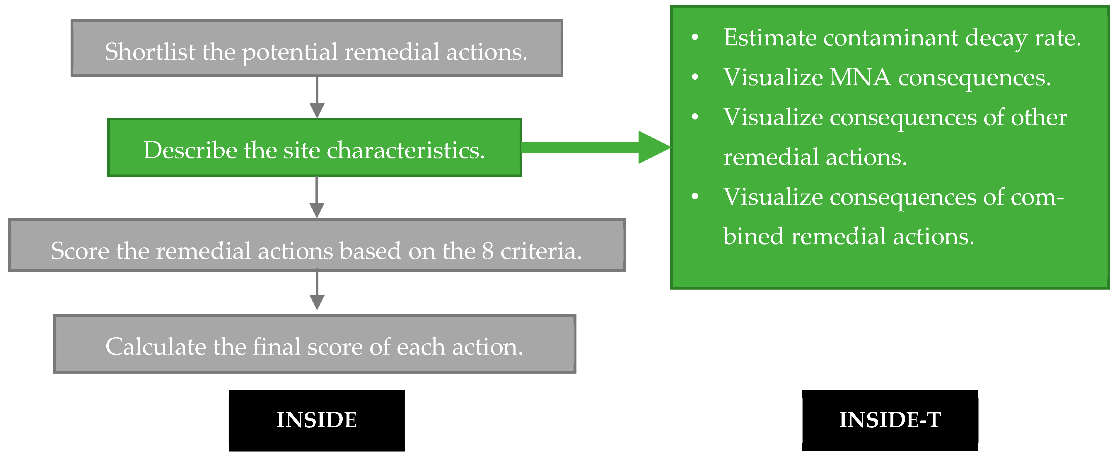
2.1. Outline of Process and Steps

INSIDE represents a DSS built to enable the participation of a diverse group of stakeholders working together to screen and preliminarily manage contaminated sites cleanup. Specifically, the DEcision MAking Trial and Evaluation Laboratory (DEMATEL) [31] and Analytic Network Process (ANP) [32] techniques were combined within INSIDE to assign weights to score sustainability criteria and overall score remediation alternatives, respectively. In a first step, all stakeholders were given the possibility to participate in assigning the weights through reflecting on their ideas about the influences of each criterion on the others. These weights were used here for scoring the sustainability of remedy measures. However, for INSIDE, only experts experienced in remediation practice participated in scoring remediation alternatives based on sustainability criteria, which requires practical knowledge from the field.

At this point, the scoring process can be substantially improved if stakeholders have a concrete picture of what consequences each remedial action have (representing performance outcomes in terms of contaminant concentrations for a potential decision; see Supplementary Materials). INSIDE-T was therefore developed to bridge this gap. It was designed as a separate module that can be easily connected to INSIDE, improving its original capabilities and thus its reliability. Figure 1 outlines the framework for INSIDE-T and its role within the INSIDE methodology.

2.2. Contaminant Decay Rate Calculation

2.2.1. Concentration Trend Analysis by Mann–Kendall Test

The slope of the best-fit line through concentration vs. time data is a measure for the long-term natural attenuation rate (this includes biological and chemical reactions or radioactive decay [33]). There are several methods for trend analysis. Of these, the Mann–Kendall test [34] was used to determine whether the time series has a monotonic increasing or decreasing trend. This test is based on the correlation between the ranks and sequences of a time series. For the time series x₁, x₂, …, x_n, the Mann–Kendall test performs [35]:

$$S={\displaystyle \sum }_{i=1}^{n-1}{\displaystyle \sum }_{j=k+1}^{n}sgn\left(x_j-x_i\right)$$

(1)

where n is the number of data points, x_i and x_j are the time series of sequence i and j (j > i) respectively, and sgn(x_j − x_i) is the sign function.

If S > 0, then later observations in the time series tend to be larger than those that appear earlier, while the reverse is true if S > 0. The variance of S is given by:

$$Var\left(S\right)=\frac{1}{18}[n\left(n-1\right)\left(2n+5\right)-{\displaystyle \sum }_{i=1}^m{t}_i\left(t_i-1\right)(2t_i+5)]$$

(2)

where m is the number of groups of tied ranks and t_i denotes the number of data in the tied group [36]. A tied group is a set of sample data having the same value. The Mann–Kendall test uses the following test statistic:

$$z=\{\begin{array}{c}\frac{S-1}{se},S>0\\ 0,S=0\\ \frac{S+1}{se},S<0\end{array}$$

(3)

where se is the square root of Var(S). Positive z indicates increasing trend while negative z shows decreasing trend.

2.2.2. Calculating Contaminant Decay Rate through Mass Flux

In the case that the trend is stable or if data show no trend, source lifetime calculations must be practiced [37]. Mass flux, due to advection, is equal to the quantity of water flow times the concentration of dissolved solids given by:

$$Mass Flux=K\frac{\Delta h}{\Delta l}A{C}_0$$

(4)

where K (L/T) is hydraulic conductivity, n_e (−) is effective porosity, d_h/d_l (L/L) is hydraulic gradient, C₀ (M/L³) is initial concentration in groundwater at the source area, and A (L²) is the cross-sectional area of groundwater flow through the source.

Source lifetimes can then be readily estimated by dividing the entire mass of the contamination at the source by the mass flux.

2.3. Contaminant Transport and Fate Modeling

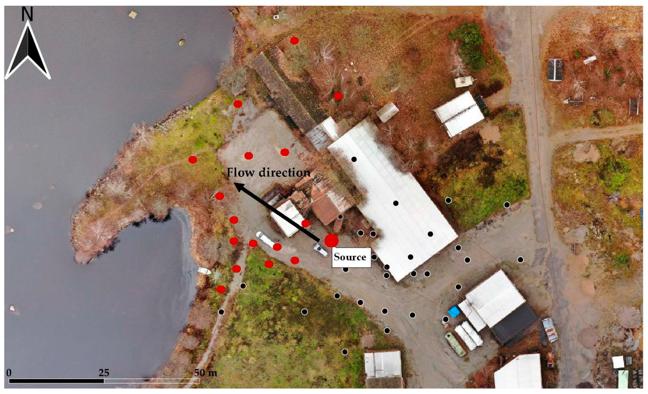
A participatory DSS like INSIDE is envisioned to be readily applied by managers and stakeholders of various backgrounds. For this purpose, the transport model should be able to simulate the concentration change reliably, addressing the associated uncertainty. Therefore, INSIDE-T was programmed in commonly used spreadsheets, and only one simple Visual Basic for Applications (VBA) Macro was used in Microsoft Excel©. The VBA Macro does parameter estimation. Parameter estimation may be defined as the determination of parameter values that govern the behavior of a system, assuming that the mechanism of the process is known [38]. In our case, this includes solving the transport problem as many times as needed to minimize the model error, on a trial-and-error basis. The error is the difference between measured and calculated values at observation points and times, which can be defined as mean absolute error or root mean square error (RMSE). Minimizing the error is done by changing the parameters involved in the transport process in their ranges until the minimum difference between modeled and measured values is reached.

After inserting observed concentration, hydraulic gradients, and locations of sampling points, a range for transport parameters (see

Table 1. Ranges of final transport parameters, their distributions, and standard deviation.

Parameter	$\mathit{T}$	$\mathit{b}$	$\mathit{K}$	ne	αL	αT	${\mathit{\rho }}_{\mathit{b}}$	Koc	foc
Unit	m	m	m/d	-	m	m	kg/L	L/kg	-
Initial Estimates
Taken from	FM	FM *	FM	FM	Lit **	Lit	FM	Lit	Lit
Min	5	3	0.04	0.25	1	αL/20	1.9	398	0.0002
Max	65	5	40	0.35	30	αL/6	2.4	19,953	0.02
Simulation Results
1st quartile	9.00	3.00	4.00	0.30	26.00	2.60	2.17	398.00	0.0034
Median	9.09	3.00	4.00	0.32	27.68	2.77	2.20	398.47	0.0103
3rd quartile	10.52	3.03	4.60	0.35	28.00	2.80	2.20	399.96	0.0187
St. dev.	0.68	0.31	0.46	0.02	0.94	0.56	0.10	0.89	0.0074

* Field measurements (FM) ** Literature (Lit) [33].

) is specified. The program then calculates the concentration at any point down-gradient of the source by modifying the parameters, according to their determined ranges, to minimize the error.

We consider the advective dispersive equation for solute transport according to [21,39,40] that is based on partial differential equations of dispersion, developed for homogeneous and isotropic media where Darcy’s law is valid:

$$D_L\frac{{\partial }^{2}C}{\partial x^2}+D_T\frac{{\partial }^{2}C}{\partial y^2}-v_x\frac{\partial C}{\partial x}=\frac{\partial C}{\partial t}$$

(5)

where C (M/L³) is solute concentration, D_L (L²/T) is longitudinal hydrodynamic dispersion, D_T (L²/T) is transverse hydrodynamic dispersion, and v_x (L/T) is the average linear velocity.

Considering the third type boundary condition (variable flux) [39], the integration of Equation (5) can be solved by Hantash (1956) [40]:

$$c\left(x,y,t\right)=\frac{C_0(\frac{Q}{b})}{4\pi {\left(D_L{D}_T\right)}^{1/2}}exp\left(\frac{v_{x}x}{2D_L}\right)\left[W\left(0,B\right)-W\left(t_D,B\right)\right]$$

(6)

while

$$t_D=\frac{{v_x}^{2}t}{4D_L} and B^2=\frac{{v_x}^2{x}^2}{4{D_L}^2}+\frac{{v_x}^2{y}^2}{4D_L{D}_T}$$

where Q (L³/T) is the rate of injected contaminant and b (L) is the thickness of the aquifer over which the contaminant is injected. Known as leaky well function, the values of W(t_D, B), and W[u, r/b] can be found in Hantush (1956) [40]. The third type boundary condition is given as:

$$-D\frac{\partial c}{\partial x}+v_{x}C=v_{x}C\left(t\right)$$

where C(t) is a known concentration function.

Involved parameters (i.e., v_x, D_L, D_T, and Q) need to be addressed prior to solving Equation (8). According to Darcy’s law, average linear velocity, v_x, is the rate at which the flux of water unidirectionally cross the unit cross-sectional area of pore space occurs [33]:

$$v_x=\frac{K}{n_e}\frac{dh}{dl}$$

(7)

However, many contaminants adsorb to the surface of soil particles while moving by groundwater flow, which results in slowing down or retarding the contaminant movement compared to groundwater. The retardation can be calculated for hydrophobic (organic) compounds as:

$$R=1+\left(\frac{{\rho }_b}{n_e}\right)K_{oc}{f}_{oc}$$

(8)

where R (−) is the retardation factor, ${\rho }_b$ (M/L³) is the bulk density of aquifer solids, K_oc (L³/M) is the organic carbon/water partition coefficient (chemical specific), and f_oc (−) is the fraction of the organic carbon content of aquifer materials.

Then, contaminant velocity, v_c, can be calculated as:

$$v_c=\frac{v_x}{R}$$

(9)

Multiplying this velocity by the cross-sectional area of the plume represents the injection rate of the contaminant (Q) to the aquifer at source:

$$Q=v_c·T·b$$

(10)

where T (L) is plume width and b (L) is the thickness of the aquifer over which the contaminant is injected.

The longitudinal and transverse hydrodynamic dispersions, D_L and D_T, can be calculated by:

$$D_L={\alpha }_L{v}_c+D^{\ast }$$

(11)

$$D_T={\alpha }_T{v}_c+D^{\ast }$$

(12)

where α_L (L²/T) is longitudinal dynamic dispersivity and α_T is (L²/T) the transverse dynamic dispersivity

The D* is the effective diffusion coefficient calculated as:

$$D^{\ast }=\omega D_d$$

(13)

where ω is a coefficient related to the tortuosity [41] and D_d is the diffusion coefficient (L²/T). However, as D_d is small and ω is always less than 1, we neglect the effective diffusion coefficient, D*. We only give measured values of the exact location of the downstream points in terms of X and Y (which stand for longitudinal and transverse distance from the source—considering flow direction, see Figure 2), contaminant concentration at source, and hydraulic gradient between any desired well and the source. Other required parameters will merely be the ranges of changes for T, b, K, n_e, α_L, α_T, ${\rho }_b$, K_oc, and f_oc. Sensitivity of these parameters will then be analyzed through the commonly used one-factor-at-a-time (OFAT) method. By OFAT, simply one parameter is adjusted at a time while all other parameters are kept fixed [42].

Parameter estimation is basically an optimization process and may be referred to as numerical, as it would not provide exact values for the best fit, which is when simulated values exactly match observed values. In that sense, INSIDE-T is semi-analytic as the parameter estimation is numeric but based on an analytic solution (Equation (6)). This analytic solution is then used for forward modeling using the estimated parameters.

INSIDE-T was applied to a case study in Sweden to illustrate the applicability in a real-world, environmental clean-up project. The model parameters used in the case study were taken either from field measurements by SGU or from relevant literature and technical reports with similar conditions. The aim was to perform an inverse modeling to estimate transport parameters, and based on that, perform a forward modeling to provide the decision-maker(s) with a reliable visualization of the potential consequences of a chosen remediation option.

2.4. Case Study

Chlorophenols were used in Sweden until 1978 for treating wood to prevent attack by discoloring fungi during storage and transport [43]. This is the source of the contamination problem at a former sawmill plant in Hjortsberga, Alvesta Municipality, Kronoberg County, southern Sweden (Figure 2). The sawmill plant was in operation from the early 1940s to the late 1970s [44] and has left a legacy of contaminated soil and groundwater with pentachlorophenol (PCP), a branch of chlorophenols. The contamination in the groundwater is threatening the nearby Lake Sjöatorpasjön. This lake is used for recreational purposes and especially swimming. Residents also farm close to the lake [44].

In 2013, a shaft remediation was implemented at this site and almost all unsaturated contaminated soil was removed with an excavator [45]. However, the PCP concentration in groundwater is still elevated and above acceptable limits [46].

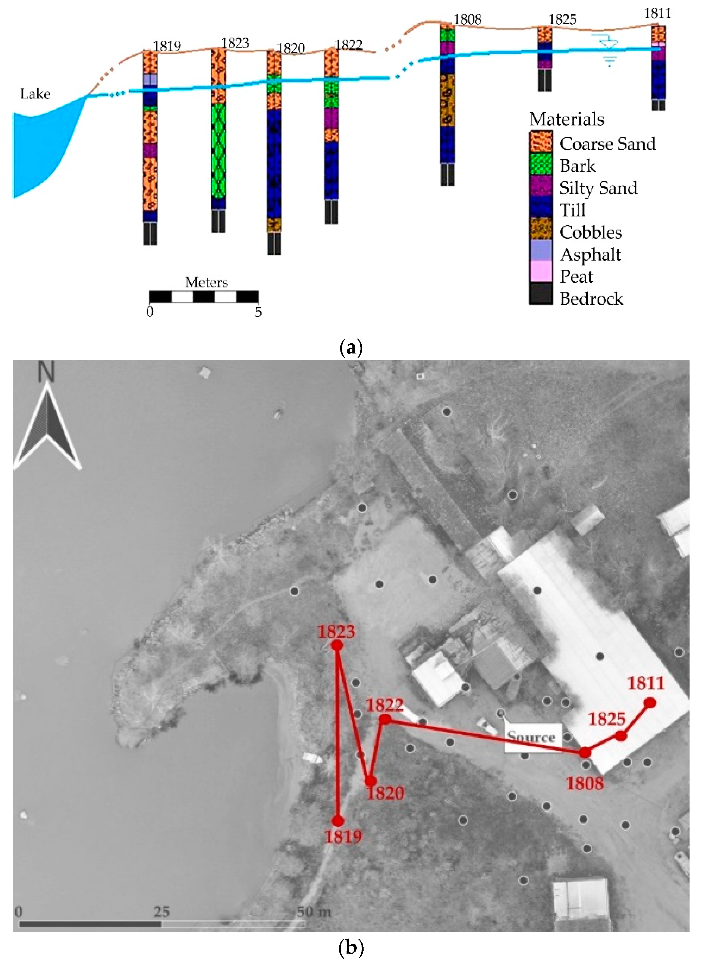
2.4.1. Geologic Media

The typical natural stratigraphy in the area is bedrock covered by till [47]. The deposits at Hjortsberga are described as “complex and heterogeneous” [45]. Geologic media at the site mainly consist of coarse-grained glaciofluvial sediments, tills with different grain size, clay, and peat (Figure 3). Commonly, the depth to bedrock is less than 5 m in the area, therefore, the surface topography reflects the bedrock [46]. The composition of the till in the region is mostly sandy-silty with a normal to low content of boulders [48]. Organic material in the form of bark (the hard, outer covering of trees) and sawdust also occurs. These deposits were produced over the decades at the sawmill [46]. The bedrock at the site is of crystalline character with water-bearing fractures in a north-northwest to south-southeast and south-southwest to north-northeast direction [48]. It should be noted that most analytical frameworks and especially the one applied here assume homogeneity of aquifer media. For screening and early management practices, these models are of great help [12,15,17] and more advanced modeling procedures would be performed in case this is needed and performing them is applicable. The methodology we used for simulating contaminant transport can estimate specific values of transport parameters for individual contaminant pathways (from source to individual wells downgradient of the source). However, for simplicity and brevity we do not provide these, and general values only are provided.

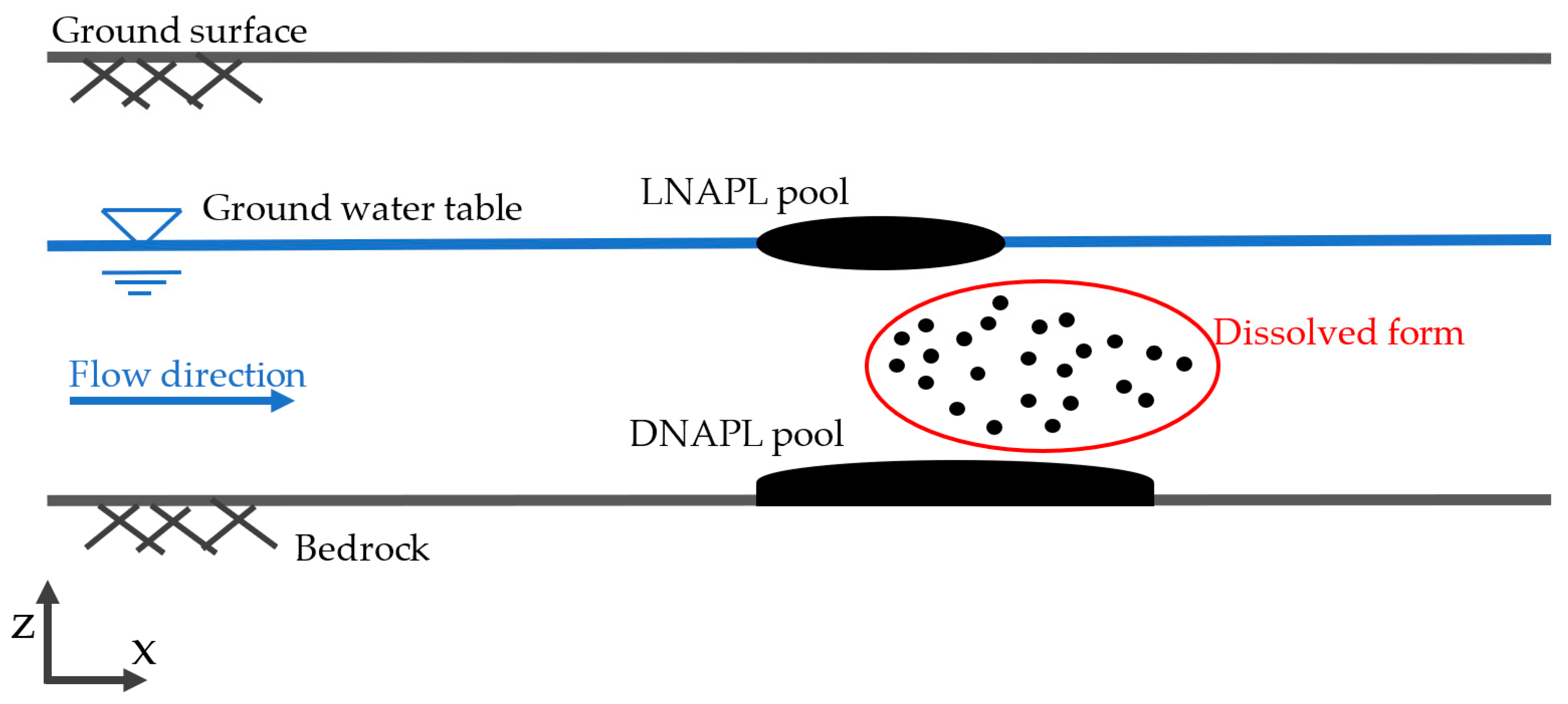
2.4.2. Contaminant Characteristics

The mobility of PCP is highly dependent on solution pH [49]. Hurst et al. (1997) showed that PCP solubility at pH 4.2 is 13.2 mg/L and at pH 7.65 it is 1465 mg/L [50]. Autochthonous microbes can remove low level PCP (<1.0 mg/L) to approach if not reach the regulatory standard of 0.001 mg/L with the addition of oxygen, with or without nutrient amendments [51].

Site investigations were performed by different consultants between January 2014 and August 2020 in 21 different sampling campaigns. There was an estimated source concentration in 2013. The number of sampling events in different years ranged from only one in 2016, 2019, and 2020 to 8 in 2018. Importantly, not all wells were sampled for all sampling events. The maximum number of samples taken from one well was 10 over the entire period, while most of the wells (points) were sampled only once or twice during this period. It is therefore not easy to uncover trends in contamination concentration change for any well. Considering third type boundary conditions, on which the chosen analytical framework was based, the initial contaminant concentration at all points must be zero at the starting time (C(x, 0) = 0). This was estimated to be the case in 1980, as site managers and early consultants’ reports suggest [45,46,49]. However, as the measured contaminant concentrations are available only since 2013, and for better visualization of scenarios, we plotted only 37 years of contaminant concentration (from 2013 to 2050). We assumed 2050 as the ending time of the simulation as it was the latest considered time of remediation of the site according to upstream regulations and targets. It should be noted that although PCP in groundwater may be in NAPL form as well [52], the form of contamination that was assessed here was the dissolved form. This was also observed in the field. Figure 4 shows a conceptual model for this.

3. Results

3.1. Implementing the Model

In total, 312 measured concentrations in the wells obtained from 2014 to 2020 were used to run the transport model, of which 208 were taken for calibration (parameter estimation) and 104 for validating the model. The calibration entailed optimizing the solution by minimizing the absolute error (difference between measured and modeled values at a certain point downstream the contamination source). For this, transport parameters were calibrated until converging to a best fit. Initial ranges of these parameters are listed in Table 1 under rows Min and Max.

Figure 5 shows observations vs. simulations for (a) calibration and (b) validation phases of the model for all measured concentrations from January 2014 to August 2020.

Moreover, we applied the Nash–Sutcliffe model efficiency coefficient (NSE) [53] to assess the predictive skill of the model. According to Moriasi et al. (2007) [54], NSE = 1.0 is the perfect fit, NSE > 0.75 is a very good, NSE = 0.64 to 0.74 is a good, NSE = 0.5 to 0.64 is a satisfactory, and NSE < 0.5 is an unsatisfactory fit. In our model, NSE was calculated to be 0.752 and 0.609 for calibration and validation results, respectively.

Descriptive statistics of final transport parameters are shown in Table 1. A small standard deviation indicates that the values tend to be close to the median, while a high standard deviation indicates that the values are spread over a wider range. Sensitivity analysis through OFAT showed that plume widths, dispersivity (both longitudinal and transverse), and partition coefficient were the most influential parameters.

Considering small standard deviation values (last row, Table 1), median values may be used as parameter values for simulating the contamination transport in the time span of interest (forward modeling). However, because of the spatial and temporal variability of these parameters [12], especially regarding the needed long-term spans of the study simulations, and due to our limited knowledge of measurements accuracy and errors, we need to deal with the inherent uncertainty in parameter values. Thus, 1st and 3rd quartile values for all transport parameters were used to suggest confidence levels for contaminant fate down-gradient of the source zone. This was to show the results in terms of most probable outcomes. According to Dekking et al. (2005) [55], the three main quartiles are 1st, 2nd, and 3rd quartiles, which were those used here. The first quartile (Q1) is defined as the middle number between the smallest (minimum) and the median of the dataset meaning that 25% of the data are below this point. The second quartile (Q2) is the median; thus 50% of the data lie below this point. The third quartile (Q3) is defined as values between the median and the maximum meaning that 75% of the data lie below this point.

The smallest distance from the source to the recipient is 60 m along the straight source-recipient line with a 2 m distance from this line (x = 60 m, y = 2 m).

3.2. Assessing MNA as a Remedial Option

To forward model contaminants transport, a PCP decay rate at the source had to be taken into consideration. This rate had to be estimated properly to develop more realistic performance outputs. The effectiveness of natural attenuation as an acceptable remedy measure is based upon decreasing contaminant concentrations in groundwater together with a stable or receding contaminant plume [56].

The Mann–Kendall test was therefore performed for PCP concentration data from wells within the source area. Results indicated that no well was showing a decreasing trend, and only a few wells were presenting probably decreasing trends. Most of them were categorized as stable or no-trend. Thus, mass flux calculation was used to estimate the source lifetime. Based on Equation (4), source lifetime was calculated with 1st, 2nd, and 3rd quartiles for transport parameters, resulting in 78, 100, and 43 years, respectively. Having a shorter source lifetime for the 3rd quartile result compared to those for 1st, and 2nd is not a surprise. Setting transport parameters corresponding to a higher percentile does not necessarily mean a higher or lower concentration downstream. This is mainly because some parameters were inversely correlated. For example, higher groundwater velocities result in further spread of contaminants but less degradation due to short time intervals [17]. We used the 2nd quartile to perform further analyses for the most conservative case scenario. By that, average groundwater velocity, contaminant velocity, and retardation are estimated as 7 × 10⁻⁴ cm/s, 2 × 10⁻⁴ cm/s, and 3.2, respectively.

Hence, based on the assumptions of 100 years as the source lifetime, the corresponding contaminant concentration decay at the source was estimated to about 10% per year. Taking this into consideration, a first scenario for monitored natural attenuation could be set up. Figure 6a depicts the uncertainty in model output at the recipient (x = 60 m, y = 2 m) from 2013 to 2050. Concentrations in the Y axis of this plot are in logarithmic scale for better visualization of lower concentrations in years.

This is, however, based on source–pathway–recipient approach, meaning that it can run for each individual point in a 2D planar view of a site and give breakthrough curves of contaminant concentrations in time and not a regional presentation of the plume. However, the model can be used together with a software that is capable of such visualizations. The inverse modeling results may give input to such a software and result in contours of iso-concentration simulated plume. We used HYDROSCAPE [15] for this purpose that was based on analytical solutions for contaminants transport and fed it with parameter values. Results of this application are shown in Figure 6b.

For the timeframe between 2013 and 2020, observed concentration at the source varied a lot as there has been some pilot test remediation performed in the field by site managers [45]. These big variations have thus resulted in seemingly big variations in the concentration at the recipient in this time period, as shown in Figure 6a. However, for the rest of the 2021 to 2050 timeframe, concentration at the source was assumed to be reduced by the estimated decay rate of 10% per year. Therefore, the simulated concentration in Figure 6a in 2013 to 2020 timeframe does not look like a reasonably smooth plot that one may expect from such an analytic framework.

Although the simulation results for MNA show a potential to reduce PCP during the coming years, this is not satisfying the site managers. The maximum permissible limit for PCP is 1 μg/L for drinking water. However, there is no plan to use the water for drinking purposes. For this reason, site managers (SGU) are looking for reaching a contaminant concentration at the recipient corresponding to about 100 μg/L. According to the model results, and accounting for uncertainty, this condition might not be reached.

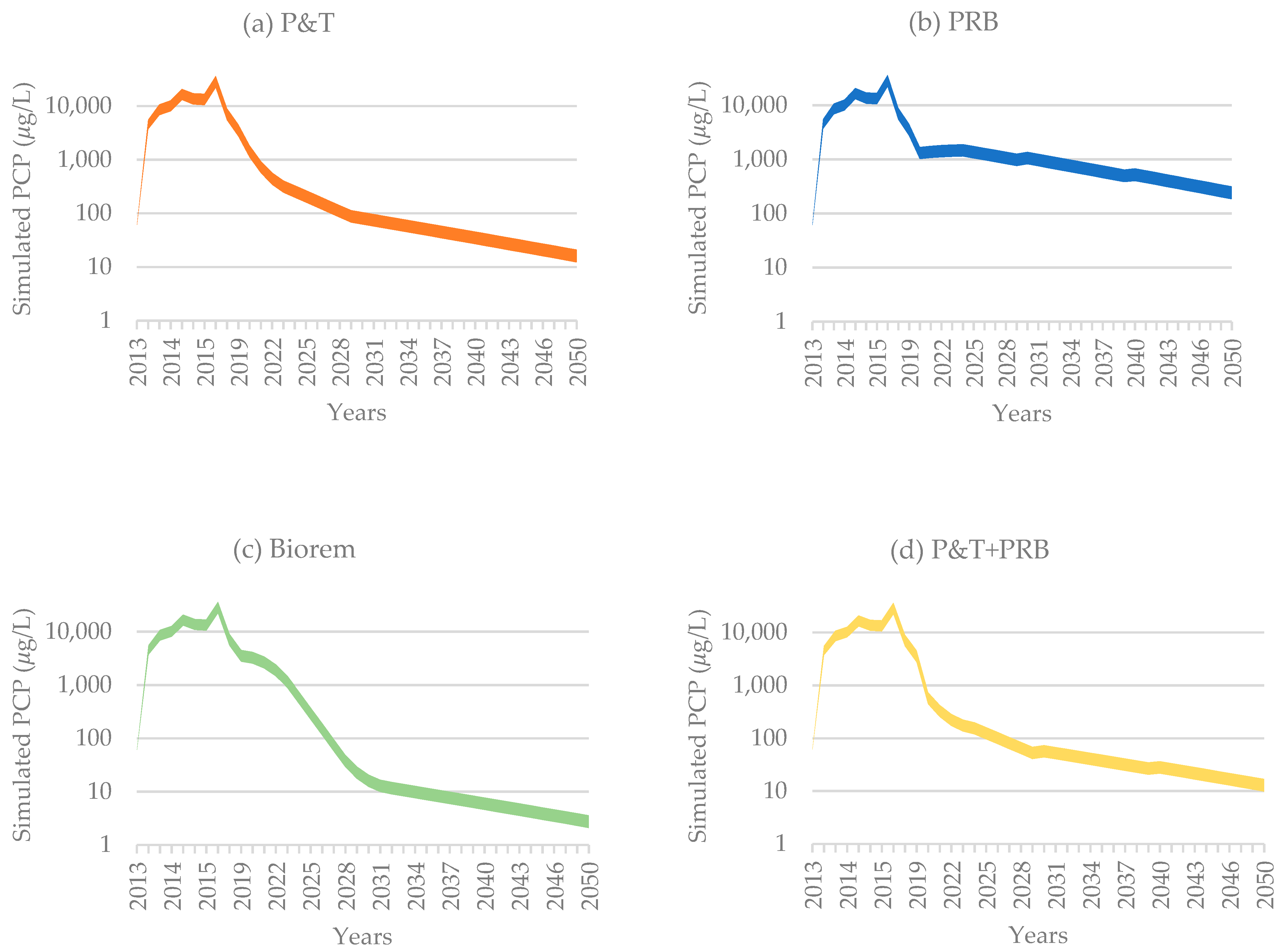
3.3. Assessing Alternative Remedial Scenarios

Shortlisted remedial methods for the site include P&T, PRB, bioremediation, and a combination of P&T and PRB. These alternatives are designated as scenarios 2 to 5, respectively. Figure 7 shows how these alternatives are likely to perform at the recipient, considering associated uncertainty.

Scenario 2, which entails P&T remediation, is meant to reduce the initial concentration at the source. Thus, the efficiency in time for P&T needs to be estimated. There are different efficiency rates for P&T in the literature for different site-specific geologic conditions. Heterogeneity of the aquifer could affect P&T efficiency substantially. However, P&T efficiency decreases significantly in time [57]. If there is still NAPL phase present, it will be much more complex than if all contaminants are in a dissolved form. NAPL will continuously partition between the NAPL phase and the dissolved phase. In addition, according to Fetter et al. (2018), it can take about 10 years to reduce the TCE concentration by 90% if the clay lens is 0.3 m thick [33]. The time increases to almost 40 years for a lens 0.6 m thick and to over 100 years for a lens 1.2 m in thickness. The same applies to other remediation methods.

Hence, we assumed reasonable efficiency rates and changes regarding these rates for all remediation alternatives based on previous studies and viewpoints of local experts with experiences in similar site conditions. Here, we used 60% efficiency for the first year of application (2021) and reduced it by 10% each year of additional application until 20% efficiency was reached in 2025. Thus, we assumed 20% reduction until 2030 and then the pumping would stop, as it would not be reasonable to keep pumping from 2030 to 2050. It should be noted that we assumed P&T and consequently a mass reduction only at the source in this scenario (Figure 7).

Figure 7 reminds us that, although we may reach lower concentrations quite early by performing P&T, the long-term performance of this technology might not be desirable nor reach the remediation target in practice. This is because P&T performance is known to decrease over time and the site characteristics are inherently uncertain (geology, source composition, etc.). From 2021 to 2030, there is only a small reduction, a function of the decreased efficiency imposed on the technology for this simulation. This is often seen for real field-scale problems [33].

A possible next scenario is to place a PRB perpendicular to the groundwater flow direction to further reduce the PCP concentration impacting the recipient. For this, we assumed that a PRB is placed 35 m downstream of the source zone to remove contaminants at a certain efficiency [46]. Johansson (2020) [46] assessed performance of a PRB at the site for different assumptions concerning width, depth, and location. Here, we assumed it is deep enough to reach the bedrock and about one meter wide. Long-term performance and removal efficiencies for this technology are, however, uncertain [58]. FRTR (2002) considers the lack of information on kinetic rates of precipitation and reactivity loss of reactive materials, and hydraulic factors (e.g., plume bypass around, under, or over the barrier, and seasonal fluctuations in groundwater flow) as the main issues affecting the performance.

Based on previous studies [33,59,60] and viewpoints of local experts, we assumed an efficiency of 60% in 2021 that would be reduced by 5% each year (to account for clogging and reactivity loss) reaching 40% in 2025. The efficiency would then be 30% and 20% for 2030s and 2040s, respectively. Figure 7b depicts the output of this scenario over the 37-year timeframe.

The PRB suggests more promising results regarding concentration reduction at the recipient. However, its performance does not result in a significant decrease in recipient concentration, because uncertainty overlaps and it is still far from the remediation target. It must be noted that placing a PRB is costly and it cannot be altered substantially after its introduction.

The next scenario considered is bioremediation (biostimulation and bioaugmentation). The efficiency of bioremediation varies for different site conditions and time [60,61]. However, to have an approximate picture of how this remedy measure may perform, we considered injecting microorganisms around the source area and if its performance changes with time. According to Schmidt et al. (1999), autochthonous microbes are capable of removing low level PCP (<1.0 mg/L). As the PCP concentration exceeds this limit, we considered a temporary decreasing contaminant removal efficiency. At first, there is too much contamination for the microorganisms to degrade, but gradually this ratio will become more balanced. After about five years, the efficiency may be considered as more or less stable [62]. Thus, we assumed that the efficiency would increase by 10% each year starting from 10% during 2021 to 50% in 2025 and then remain constant until 2050. Figure 7c depicts the simulation results for this remediation alternative. As the figures shows, we may reach the treatment target by 2026–2027, but high uncertainty in this method together with the model uncertainty may hinder its reliability.

The last scenario considered is a combination of two previously simulated remediation techniques. Thus, we assumed performing P&T at the source and placing a PRB 35 m downstream of the source. The same efficiencies were applied as when they were individually evaluated. Figure 7d illustrates the performance of this combination. However, high costs may apply, which must be considered in the decision-making process.

4. Discussion

Expectedly, all simulation scenarios considered here showed a rapid contaminant concentration reduction in the first years. The attenuation over time continues until contamination at the recipient reaches about 100 μg/L by 2050. However, this long period is not acceptable for the site managers (SGU). P&T could satisfy the desired concentration target of 100 μg/L by 2027–2031. It should be noted that presence of NAPL may require us to keep pumping for a long time. Otherwise, the concentrations will return to similar values above the required threshold. This corresponds to the rebounding phenomena that is addressed in the literature, especially for more heterogeneous geologic media [33]. However, costs may be reduced by maximizing efficiency and using intermittent P&T.

Alternatively, placing a PRB may hardly allow the goal to be reached by about 2050, which is not acceptable. A major reason for this is the efficiency reduction, e.g., due to clogging. Moreover, a detailed groundwater flow model would be needed to ensure proper placement of the PRB at the site [46]. Bioremediation is, however, even harder to predict. It depends on many factors that are difficult to control, as it deals with microorganisms. Moreover, site managers have already performed an unsuccessful pilot test at the site and are thus wary of the high risk of failure that seems to be associated with selecting this option. However, the pilot test was based on biostimulation which means stimulating existing bacteria in the environment, mostly by injecting air, to consume more contaminants. After assessment and performing a pilot test, it was concluded that, indigenous bacteria are not enough [45]. Bioaugmentation is another way of bioremediation which introduces more archaea or bacteria culture to the environment to enhance contaminants biodegradation. Nevertheless, bioaugmentation performs well in assessments and may reach treatment goals by 2026–2027, considering its noticeably low cost compared to the PRB or long-term application of P&T (cost data not shown).

Combining the two methods of P&T and PRB appears more promising, showing potential for reaching treatment goals by 2024–2027. This combination lets the P&T stop after some years (5 years were assumed in the simulation) and lets the PRB finish the remediation. This may substantially reduce the energy consumption and costs of P&T. However, considering additional costs for treating the pumped water, the overall costs of such practices might still be high.

In summary, considering the managers’ time limitations for making the lake publicly available again, simulated contaminant reduction at the recipient after five years of application was chosen for evaluating the different scenarios against the required remediation target. By 2025, concentration at the recipient would be around 100 μg/L for both Biorem and the combination of P&T with PRB. Individual applications of P&T and PRB would follow as 3rd and 4th ranked, respectively, and MNA would stand at the 5th rank.

It should be highlighted that the simulation results are associated with uncertainty. Nevertheless, the results can be used to give a first impression of what may be expected in terms of performance capabilities for different remediation strategies. Costs and other uncertainties associated with the remedial measures need to be estimated. Here, a link between INSIDE-T and INSIDE may come into play to assist site managers considering other aspects.

We provided three experienced site managers, who were already familiar with the site characteristics, with more detailed information and our simulation results, to assign grades from 1 to 9 to each remedy option for each sustainability criterion (Supplementary Materials). According to this scoring, MNA got the highest rank in sustainability, scoring 26.2 out of 100 and bioremediation was 2nd in rank, scoring 22.1. P&T (19.6), P&T + PRB (16.3), and PRB (15.7) were ranked 3rd to 5th in terms of sustainability considerations, respectively. However, for time limitation, MNA is not a feasible option and bioremediation is considered as the best option for the site. This reaffirms many recent studies (e.g., [63]) that argue less intensive remedies measured like MNA and bioremediation are more sustainable in general terms. However, the site-specific simulations that INSIDE-T provides give more confidence to decision-makers to trust the outcome of sustainability assessment tool. Careful attention was paid to make INSIDE-T simple enough for communication with users, from different backgrounds and perspectives, who need to understand the underlying mechanism of the DSS.

5. Conclusions

Variability, complexity, and uncertainty of remediation processes is too high to be simulated accurately and confidently enough at early managerial stages. Such simulations cannot be handled by a single or even a set of disciplines purely objectively. There must be room for managers’ judgments and considerations based on their experience in similar applications. This has been proven to be a must have for a sustainable remediation practice [30,63,64,65,66,67]. Our study, however, provides this room. INSIDE-T shows all the data and processes in a contaminant transport model in the most transparent way (spreadsheets, [68]) to let the manager(s) incorporate their judgements and considerations about the efficiency of remediation scenarios. After all, the transport model and adapted DSS can provide decision-makers with more reliable hydrogeological insights at the screening and preliminary management stage, and thereby enhance the overall sustainability scoring of potential remediation options. The transport module was developed in close collaboration with SGU, the site manager responsible for orphaned contaminated sites in Sweden. In this way researchers can collaborate with practitioners to develop tools in the context of (best) practice.

To this end, INSIDE-T simulates contaminant transport as a result of potential remedy actions, which may be assessed individually or in combination, including accounting for uncertainty. Simulation outcomes of INSIDE-T are contaminant concentration at the recipient for each scenario and the concentration change pattern at any selected source-to-recipient location. Site managers can develop and simulate different remediation scenarios, regardless of their level of expertise, and visualize how a particular option may affect the desired (management) outcome, i.e., concentration at the recipient. Incorporation of transport modeling can, thus, lead to a more reliable scoring of different options, based on the full set of sustainability criteria, while enabling a more transparent decision-making process.

The new tool was applied to a groundwater site in south Sweden contaminated with pentachlorophenol. Simulation scenarios were developed to enable comparison of various remediation strategies, which indicated that:

• MNA is not a viable option for the site in terms of the accepted remediation timeframe;
• a combination of P&T with PRB would be almost as effective as bioremediation, assuming five years after implementation as the cut-off point for the simulated concentration reduction at the recipient; and
• these insights can help site managers in developing and selecting sustainable remediation strategies.

Another merit of this kind of simple solution is its adaptability with a limited number of observations. Detailed and costly site investigations are not possible for all contaminated sites that need remediating. Using INSIDE-T with small data needs makes regional and national remediation plans possible. More sophisticated modeling tools can then be applied as needed. Results of such advanced models can be used to inform and update INSIDE-T, i.e., for better calibration and leading to more reliable outcomes.

In this study, a model was introduced that was performed in a simple way with emphasis on its transparency in all levels. Spreadsheets provided this transparency by directly showing all input and outputs in all steps and allowing the users to analyze different scenarios in these steps (e.g., at the source, in plume, and by variable efficiency rates). Because of such availability, this model can fit into many further applications in sustainable remediation practice. However, there are, as expected, some limitations that should be noted before application. Although simplicity is a merit for such tools, it could cause problems if the site complexity (hydrogeochemical conditions) is not properly represented by the collected data. As with all modeling tools, site investigations must be performed to give basic information on transport properties to tackle this issue. In addition, although careful attention was paid to make efficiency assumptions when visualizing scenarios, these may not reflect the true performance efficiency in the field, nor may these assumptions be directly transferred to different sites, as treatment performance efficiencies are expected to be site-specific. INSIDE-T nevertheless represents an advancement for addressing the technical issues and uncertainties typically associated with remediation planning and management, as identified by previous applications of the INSIDE DSS.

References

1. Hou, D.; Li, F. Complexities Surrounding China’s Soil Action Plan. Land Degrad. Dev. 2017, 28, 2315–2320. [Google Scholar] [CrossRef] [Green Version]
2. Suthersan, S.S.; Horst, J.; Schnobrich, M.; Welty, N.; McDonough, J. Remediation Engineering, Design Concepts, 2nd ed.; CRC Press, Taylor & Francis Group: Boca Raton, FL, USA, 2017. [Google Scholar]
3. Palma, V.; Accorsi, F.; Casasso, A.; Bianco, C.; Cutrì, S.; Robiglio, M.; Tosco, T. AdRem: An Integrated Approach for Adaptive Remediation. Sustainability 2021, 13, 28. [Google Scholar] [CrossRef]
4. Maskooni, E.K.; Naseri-rad, M.; Berndtsson, R.; Nakagawa, K. Use of Heavy Metal Content and Modified Water Quality Index to Assess Groundwater Quality in a Semiarid Area. Water 2020, 12, 1115. [Google Scholar] [CrossRef] [Green Version]
5. Chowdhury, S.; Kain, J.-H.; Adelfio, M.; Volchko, Y.; Norrman, J. Greening the Browns: A Bio-Based Land Use Framework for Analysing the Potential of Urban Brownfields in an Urban Circular Economy. Sustainability 2020, 12, 6278. [Google Scholar] [CrossRef]
6. Lemming, G.; Chambon, J.C.; Binning, P.J.; Bjerg, P.L. Is there an environmental bene fi t from remediation of a contaminated site? Combined assessments of the risk reduction and life cycle impact of remediation. J. Environ. Manag. 2012, 112, 392–403. [Google Scholar] [CrossRef]
7. Norrman, J.; Söderqvist, T.; Volchko, Y.; Back, P.; Bohgard, D.; Ringshagen, E.; Svensson, H.; Englöv, P.; Rosén, L. Enriching social and economic aspects in sustainability assessments of remediation strategies—Methods and implementation. Sci. Total Environ. 2020, 707, 136021. [Google Scholar] [CrossRef]
8. Swedish EPA. Lägesbeskrivning av Efterbehandlingsarbetet i Landet (Situation Description of the Decontamination Work in the Country); Swedish EPA: Stockholm, Sweden, 2008.
9. Swedish EPA. Lägesbeskrivning av Arbetet Med Efterbehandling av Förorenade Områden (Situation Description of the Work with Decontamination of Contaminated Areas). Available online: https://www.naturvardsverket.se/upload/sa-mar-miljon/mark/fororenade-omraden/lagesbeskrivning-20170413.pdf (accessed on 18 October 2020).
10. Forslund, J.; Samakovlis, E.; Johansson, M.V.; Barregard, L. Does remediation save lives?—On the cost of cleaning up arsenic-contaminated sites in Sweden. Sci. Total Environ. 2010, 408, 3085–3091. [Google Scholar] [CrossRef] [Green Version]
11. Vredin Johansson, M.; Forslund, J.; Johansson, P.; Samakovlis, E. Can we buy time? Evaluation of the Swedish government’s grant to remediation of contaminated sites. J. Environ. Manag. 2011, 92, 1303–1313. [Google Scholar] [CrossRef]
12. McKnight, U.S.; Finkel, M. A system dynamics model for the screening-level long-term assessment of human health risks at contaminated sites. Environ. Model. Softw. 2013, 40, 35–50. [Google Scholar] [CrossRef]
13. Marcomini, A.; Suter, W.G., II; Critto, A. Decision Support Systems for Risk-Based Management of Contaminated Sites; Springer Science & Business Media, LLC: Berlin/Heidelberg, Germany, 2009; ISBN 9780387097213. [Google Scholar]
14. Bardos, R.P.; Bakker, L.M.M.; Slenders, H.L.A.; Nathanail, C.P. Sustainability and Remediation BT—Dealing with Contaminated Sites: From Theory towards Practical Application; Swartjes, F.A., Ed.; Springer: Dordrecht, The Netherlands, 2011; pp. 889–948. ISBN 978-90-481-9757-6. [Google Scholar]
15. Funk, S.P.; Hnatyshin, D.; Alessi, D.S. HYDROSCAPE: A new versatile software program for evaluating contaminant transport in groundwater. SoftwareX 2017, 6, 261–266. [Google Scholar] [CrossRef]
16. McKnight, U.S.; Funder, S.G.; Rasmussen, J.J.; Finkel, M.; Binning, P.J.; Bjerg, P.L. An integrated model for assessing the risk of TCE groundwater contamination to human receptors and surface water ecosystems. Ecol. Eng. 2010, 36, 1126–1137. [Google Scholar] [CrossRef] [Green Version]
17. Locatelli, L.; Binning, P.J.; Sanchez-vila, X.; Lemming, G.; Rosenberg, L.; Bjerg, P.L. A simple contaminant fate and transport modelling tool for management and risk assessment of groundwater pollution from contaminated sites. J. Contam. Hydrol. 2019, 221, 35–49. [Google Scholar] [CrossRef] [PubMed]
18. Zheng, C.; Bennett, G.D. Applied Contaminant Transport Modeling, 2nd ed.; Wiley-Interscience: New York, NY, USA, 2002; Volume 2. [Google Scholar]
19. Harclerode, M.A.; Macbeth, T.W.; Miller, M.E.; Gurr, C.J.; Myers, T.S. Early decision framework for integrating sustainable risk management for complex remediation sites: Drivers, barriers, and performance metrics. J. Environ. Manag. 2016, 184, 57–66. [Google Scholar] [CrossRef] [PubMed]
20. Ogata, A.; Banks, R.B. A Solution of the Differential Equation of Longitudinal Dispersion in Porous Media; US Government Printing Office: Washington, DC, USA, 1961.
21. Ogata, A. Theory of Dispersion in a Granular Medium; US Government Printing Office: Washington, DC, USA, 1970.
22. Wexler, E.J. Analytical Solutions for One-, Two-, and Three-Dimensional Solute Transport in Ground-Water Systems with Uniform Flow; US Government Printing Office: Washington, DC, USA, 1992.
23. Bauer, P.; Attinger, S.; Kinzelbach, W. Transport of a decay chain in homogenous porous media: Analytical solutions. J. Contam. Hydrol. 2001, 49, 217–239. [Google Scholar] [CrossRef]
24. Sudicky, E.A.; Hwang, H.-T.; Illman, W.A.; Wu, Y.-S.; Kool, J.B.; Huyakorn, P. A semi-analytical solution for simulating contaminant transport subject to chain-decay reactions. J. Contam. Hydrol. 2013, 144, 20–45. [Google Scholar] [CrossRef]
25. Paladino, O.; Moranda, A.; Massabò, M.; Robbins, G.A. Analytical Solutions of Three-Dimensional Contaminant Transport Models with Exponential Source Decay. Groundwater 2018, 56, 96–108. [Google Scholar] [CrossRef]
26. Newell, C.J.; McLeod, R.K.; Gonzales, J.R. BIOSCREEN, Natural Attenuation Decision Support System; Version 1.4; United States Environmental Protection Agency, Office of Research and Development: Washington, DC, USA, 1997.
27. Aziz, C.E.; Newell, C.J.; Gonzales, J.R. BIOCHLOR, Natural Attenuation Decision Support System; Version 2.2; United States Environmental Protection Agency, Office of Research and Development: Washington, DC, USA, 2002.
28. Falta, R.W.; Ahsanuzzaman, A.N.M.; Stacy, M.B.; Earle, R.C. REMFuel, Remediation Evaluation Model for Fuel Hydrocarbons; Version 1.0; United States Environmental Protection Agency, Office of Research and Development: Washington, DC, USA, 2012.
29. Falta, R.W.; Stacy, M.B.; Ahsanuzzaman, A.N.M. REMChlor, Remediation Evaluation Model for Chlorinated Solvents; Version 1.0; United States Environmental Protection Agency, Office of Research and Development: Washington, DC, USA, 2007.
30. Naseri-Rad, M.; Berndtsson, R.; Persson, K.M.; Nakagawa, K. INSIDE: An efficient guide for sustainable remediation practice in addressing contaminated soil and groundwater. Sci. Total Environ. 2020, 740, 139879. [Google Scholar] [CrossRef]
31. Gabus, A.; Fontela, E. World Problems an Invitation to Further Thought within the Framework of DEMATEL; Batelle Institute, Geneva Research Center: Geneva, Switzerland, 1972. [Google Scholar]
32. Saaty, T.L. Decision Making with Dependence and Feedback: The Analytic Network Process; RWS Publications: Pittsburgh, PA, USA, 1996. [Google Scholar]
33. Fetter, C.W.; Boving, T.; Kreamer, D. Contaminant Hydrogeology, 3rd ed.; Waveland Press, Inc.: Long Grove, IL, USA, 2018; ISBN 9781478632795. [Google Scholar]
34. Mann, H.B. Nonparametric Tests against Trend. Econometrica 1945, 13, 245–259. [Google Scholar] [CrossRef]
35. Gocic, M.; Trajkovic, S. Analysis of changes in meteorological variables using Mann-Kendall and Sen’s slope estimator statistical tests in Serbia. Glob. Planet. Chang. 2013, 100, 172–182. [Google Scholar] [CrossRef]
36. Wang, F.; Shao, W.; Yu, H.; Kan, G.; He, X.; Zhang, D.; Ren, M.; Wang, G. Re-evaluation of the Power of the Mann-Kendall Test for Detecting Monotonic Trends in Hydrometeorological Time Series. Front. Earth Sci. 2020, 8, 14. [Google Scholar] [CrossRef]
37. United States Environmental Protection Agency Chapter IX, Monitored Natural Attenuation. In How to Evaluate Alternative Cleanup Technologies for Underground Storage Tank Sites; United States Environmental Protection Agency, Land and Emergency Management: Washington, DC, USA, 2017.
38. Avula, X.J.R. Mathematical Modeling. In Encyclopedia of Physical Science and Technology, 3rd ed.; Meyers, R.A., Ed.; Academic Press: New York, NY, USA, 2003; pp. 219–230. ISBN 978-0-12-227410-7. [Google Scholar]
39. Freeze, R.A.; Cherry, J.A. Groundwater; Prentice-Hall: Hoboken, NJ, USA, 1979; ISBN 9780133653120. [Google Scholar]
40. Bear, J. Dynamics of Fluids in Porous Media; Dover: New York, NY, USA, 1988; ISBN 0486656756. [Google Scholar]
41. Van Genuchten, M.T. Analytical solutions for chemical transport with simultaneous adsorption, zero-order production and first-order decay. J. Hydrol. 1981, 49, 213–233. [Google Scholar] [CrossRef]
42. Hantush, M.S. Analysis of data from pumping tests in leaky aquifers. Eos, Trans. Am. Geophys. Union 1956, 37, 702–714. [Google Scholar] [CrossRef]
43. Li, Z.; Chen, B.; Wu, H.; Ye, X.; Zhang, B. A design of experiment aided stochastic parameterization method for modeling aquifer NAPL contamination. Environ. Model. Softw. 2018, 101, 183–193. [Google Scholar] [CrossRef]
44. Swedish EPA. The Role of Pentachlorophenol Treated Wood for Emissions of Dioxins into the Environment. Available online: https://www.naturvardsverket.se/Documents/publikationer/978-91-620-5935-4.pdf?pid=3534 (accessed on 18 October 2020).
45. Elander, P.; Eriksson, H. Södra Skogsägarna Hjortsberga f.d. Sågverk Fördjupad Riskbedömning och Åtgärdsutredning (In-Depth risk Assessment and Action Investigation Report for Southern Hjortsberga Former Sawmill). Available online: https://www.lansstyrelsen.se/download/18.76f16c3d1665eba4c3e50bc/1539688734395/Fördjupadriskbedömningochåtgärdsutredning,Envipro2007pdf (accessed on 18 October 2020).
46. Nord, H. Provtagningar och Undersökningar av Grundvatten, Sediment, Ytvatten och Dehalococoider (Sampling and Investigations of Groundwater, Sediment, Surface Water and Dehalococoids); RGS Nordic: Stockholm, Sweden, 2019. [Google Scholar]
47. Johansson, A. Groundwater Flow Modelling to Address Hydrogeological Response of a Contaminated Site to Remediation Measures at Hjortsberga, Southern Sweden. Bachelor’s Thesis, Lund University, Lund, Sweden, 2020. [Google Scholar]
48. Axelsson, P.; Håkansson, K. Hjortsberga såg, Undersökningsrapport Avseende Åtgärdsförberedande Undersökningar (Hjortsberga sawmil, Investigation Report Regarding Action-Preparatory Investigations); LÄNSSTYRELSEN: Stockholm, Sweden, 2012. [Google Scholar]
49. Johansson, L. Södra Skogsägarna Ekonomisk Förening. Utökad Undersökning vid Hjortsberga Sågverk (Southern Forest Owners Cooperative Society. Extended Investigation at Hjortsberga Sawmill). Available online: https://www.lansstyrelsen.se/download/18.4e0415ee166afb59324449/1540558355286/S%C3%A5gverkiHjortsberga-Ut%C3%B6kadunders%C3%B6kning,SWECOVIAK2006.pdf (accessed on 18 October 2020).
50. Liu, F.; Xu, B.; He, Y.; Brookes, P.C.; Xu, J. Co-transport of phenanthrene and pentachlorophenol by natural soil nanoparticles through saturated sand columns. Environ. Pollut. 2019, 249, 406–413. [Google Scholar] [CrossRef]
51. Hurst, C.J.; Sims, C.R.; Sims, L.J.; Sorensen, L.D.; McLean, E.J.; Huling, S. Soil Gas Oxygen Tension and Pentachlorophenol Biodegradation. J. Environ. Eng. 1997, 123, 364–370. [Google Scholar] [CrossRef]
52. Schmidt, L.M.; Delfino, J.J.; Preston, J.F., 3rd; St Laurent, G., 3rd. Biodegradation of low aqueous concentration pentachlorophenol (PCP) contaminated groundwater. Chemosphere 1999, 38, 2897–2912. [Google Scholar] [CrossRef]
53. Rao, M.A.; Di Rauso Simeone, G.; Scelza, R.; Conte, P. Biochar based remediation of water and soil contaminated by phenanthrene and pentachlorophenol. Chemosphere 2017, 186, 193–201. [Google Scholar] [CrossRef]
54. Nash, J.E.; Sutcliffe, J.V. River flow forecasting through conceptual models part I—A discussion of principles. J. Hydrol. 1970, 10, 282–290. [Google Scholar] [CrossRef]
55. Moriasi, D.N.; Arnold, J.G.; Van Liew, M.W.; Bingner, R.L.; Harmel, R.D.; Veith, T.L. Model Evaluation Guidelines for Systematic Quantification of Accuracy in Watershed Simulations. Trans. ASABE 2007, 50, 885–900. [Google Scholar] [CrossRef]
56. WNR. Guidance on Natural Attenuation for Petroleum Releases; Wisconsin Department of Natural Resources, WNR: Madison, WI, USA, 2014.
57. Dekking, F.M.; Kraaikamp, C.; Lopuhaä, H.P.; Meester, L.E. A Modern Introduction to Probability and Statistics: Understanding Why and How; Springer: New York, NY, USA, 2005. [Google Scholar]
58. Mackay, D.M.; Cherry, J.A. Groundwater contamination: Pump-and-treat remediation. Environ. Sci. Technol. 1989, 23, 630–636. [Google Scholar] [CrossRef]
59. Obiri-Nyarko, F.; Grajales-Mesa, S.J.; Malina, G. An overview of permeable reactive barriers for in situ sustainable groundwater remediation. Chemosphere 2014, 111, 243–259. [Google Scholar] [CrossRef]
60. FRTR. Evaluation of Permeable Reactive Barrier Performance; Federal Remediation Technologies Roundtable (FRTR): USA, 2002. Available online: https://frtr.gov/pdf/2-prb_performance.pdf (accessed on 7 July 2021).
61. McGuire, T.M.; Adamson, D.T.; Burcham, M.S.; Bedient, P.B.; Newell, C.J. Evaluation of Long-Term Performance and Sustained Treatment at Enhanced Anaerobic Bioremediation Sites. Groundw. Monit. Remediat. 2016, 36, 32–44. [Google Scholar] [CrossRef]
62. Loehr, R.C.; Webster, M.T. Performance of long-term, field-scale bioremediation processes. J. Hazard. Mater. 1996, 50, 105–128. [Google Scholar] [CrossRef]
63. Guerin, T.F. Long-term performance of a land treatment facility for the bioremediation of non-volatile oily wastes. Resour. Conserv. Recycl. 2000, 28, 105–120. [Google Scholar] [CrossRef]
64. Hou, D. Sustainable Remediation of Contaminated Soil and Groundwater: Materials, Processes, and Assessment; Butterworth-Heinemann, An Imprint of Elsevier; Elsevier: Amsterdam, The Netherlands, 2020; ISBN 012817983X. [Google Scholar]
65. Rosén, L.; Back, P.-E.; Söderqvist, T.; Norrman, J.; Brinkhoff, P.; Norberg, T.; Volchko, Y.; Norin, M.; Bergknut, M.; Döberl, G. SCORE: A novel multi-criteria decision analysis approach to assessing the sustainability of contaminated land remediation. Sci. Total Environ. 2015, 511, 621–638. [Google Scholar] [CrossRef] [PubMed]
66. Li, X.; Li, J.; Sui, H.; He, L.; Cao, X.; Li, Y. Evaluation and determination of soil remediation schemes using a modi fi ed AHP model and its application in a contaminated coking plant. J. Hazard. Mater. 2018, 353, 300–311. [Google Scholar] [CrossRef]
67. Hou, D.; Ding, Z.; Li, G.; Wu, L.; Hu, P.; Guo, G.; Wang, X.; Ma, Y.; Connor, D.O.; Wang, X. A sustainability assessment framework for agricultural land remediation in China. Land Degrad. Dev. 2018, 29, 1005–1018. [Google Scholar] [CrossRef]
68. Radelyuk, I.; Naseri-Rad, M.; Hashemi, H.; Persson, M.; Berndtsson, R.; Yelubay, M.; Tussupova, K. Assessing data-scarce contaminated groundwater sites surrounding petrochemical industries. Environ. Earth. Sci. 2021, 80, 351. [Google Scholar] [CrossRef]
Figure 1. Framework of the methodology applied in this paper for INSIDE-T (green boxes) as a part of the structure of the main DSS (INSIDE) (gray boxes).
Sustainability 13 07596 g001
Figure 2. Location of the former sawmill plant and sampling wells (all dots). Red dots show wells from which data are used in this study.
Sustainability 13 07596 g002
Figure 3. (a) Topography and geologic materials, and (b) plan view location of selected boreholes at the field site (m).
Sustainability 13 07596 g003
Figure 4. Conceptual model of PCP transport in subsurface and its different forms: dense NAPL, light NAPL, and dissolved in water. The dissolved form moves with flow form the source towards downstream recipients, which is a lake in the case study.
Sustainability 13 07596 g004
Figure 5. Correlation between observations and simulation values for (a) calibration with 208 and (b) validation with 104 data points (from January 2014 to July 2020).
Sustainability 13 07596 g005
Figure 6. (a) simulation result for monitored natural attenuation (MNA) over a 37-year period, (b) iso-concentration simulated plume lines, made using HYDROSCAPE, for spatial visualization of the plume (unit: μg/L). Observed values existed only for time period 2013 to 2020.
Sustainability 13 07596 g006
Figure 7. Performance of different scenarios at the recipient in different years, considering associated uncertainty, for (a) P&T, (b) PRB, (c) Biorem, and (d) P&T + PRB. Concentrations are shown in a logarithmic scale.
Sustainability 13 07596 g007