Effects of Different Aboveground Structural Parts of Grass Strips on the Sediment-Trapping Process

Abstract

Grass strips can decrease erosion, trap sediment in silt-laden water flowing downhill, and control nonpoint source pollution. Determining the effects of different parts of grass strips on silt-laden overland flow will improve our understanding of sediment trapping by grass strips with different structures. Sediment trapping by grass strips was studied using a 5° slope, 30 L min⁻¹ m⁻¹ flow rate, 120 g L⁻¹ sediment concentration, and different aboveground components of grass strips (complete grass, removed green grass, and removed green and withered grass). The whole overland flow process was monitored. Meanwhile, the runoff sediment samples at the outlet were collected and measured. Sediment trapping by aboveground grass parts was quantified at different stages. Of the soil bed surface, green grass, and withered grass, the soil bed surface dominated sediment trapping in the initial stage of the sediment-trapping process, contributing about 90% of total sediment deposition in the first 5 min. As the sediment-trapping process continued, the effect of the soil bed surface weakened, and the green grass played a major role at the later stage of sediment trapping. The ratio of the soil bed surface, green grass, and withered grass contributions to total sediment deposition at the stable stage of the experiments was approximately 3:5:2. The results will help assess the effects of vegetation restoration on sediment transport in entire watersheds.

1. Introduction

The main way desertification/land degradation can be prevented or reversed is by increasing or at least maintaining vegetation cover [1]. The “Grain for Green” project, part of the Chinese sustainable development strategy, has been running for 20 years, and the area covered by forest or grass has been effectively restored by natural enclosure or artificial planting. A grass strip can improve the roughness of a hillslope surface and increase resistance to silt-laden overland flow [2,3]. Grass stalks, litter, the soil surface microtopography, small gravel particles (~0.5 mm diameter), and small stones all play important roles in the processes through which grass strips trap sediment [4,5].

The sediment-trapping efficiency is the percentage of the total amount of sediment flowing into a grass strip that is trapped [6]. Additionally, the sediment-trapping efficiency is determined by overland flow rate, sediment concentration, particle size, topography, and vegetation characteristics [7]. The sediment-trapping effect of a grass strip is often simply described using an overall sediment-trapping efficiency for a certain period [8], but this does not indicate temporal variations in sediment trapping by the grass strip [9]. The instantaneous sediment-trapping efficiency (ISTE) of a grass strip is usually used to indicate the real-time sediment-trapping performance of a grass strip [10,11]. The ISTE will change mainly because deposited sediment will affect the roughness of the grassland and the resistance of the grassland to overland flow [7,12]. Resistance to overland flow will be provided by all types of soil surface roughness, including vegetation, small stones, bumps, and small granules on the soil surface. The roughness of a hillslope can therefore be considered to be a composite roughness similar to riverbed roughness [13]. Since the rough elements are superimposed, the flow shear forces exerted on different rough elements in the same region can also be superimposed [14]. Weltz et al. performed simulated rainfall experiments on natural pasture containing shrubs and grass strips in the western United States and found, from the stackable principle for hillslope resistance, that the effective Darcy–Weisbach resistance factor f_e can be divided into four parts, each part representing the contribution of certain surface characteristics to overland flow resistance [4,15], as shown in Equation (1).

$$f_e=f_{rs}+f_{rr}+f_{gc}+f_{pb}$$

(1)

where f_rs, f_rr, f_gc, and f_pb are the resistances of soil, microtopography, surface cover (including the small gravels and litter that may exist on some hillslope), and standing vegetation, respectively.

Ding et al. used a 5 m long and 0.38 m wide trough to conduct the experiments of Pinus tabulaeformis litter covering conditions with 7 gradients in the range of 0–70% [16]. Compared with Mu et al. under the conditions of artificial stem mulching with nine gradients in the range of 0–30% in the same trough [17], the results show that the effect of stem on the kinetic energy of the overland flow is stronger than that of litter. Stable beds unaffected by erosion or deposition have often been used to study the effects of vegetation and bed roughness on the overland flow [16,18]. Real soil slopes have been used to study interactions between vegetation cover, erosion, and overland flow [19,20]. These studies were mainly focused on vegetation improves interception, increases infiltration, reduces soil erosion, and weakens sediment transport capacity of overland flow. Under natural conditions, the inflow of a field will usually carry sediment, and the conditions will vary according to the soil and precipitation characteristics uphill. Erosion or deposition may occur when silt-laden water flows into a vegetation area. Additionally, when sediment deposition occurs, both the hydraulic condition of vegetation-covered hillslope and the role of the soil bed micromorphology are still not well understood.

The aboveground part of a grass strip will cause flow resistance on the slope and can be divided into three main parts—green grass, withered grass, and the soil bed surface. Therefore, more energy in silt-laden flow will be lost to a grass strip than to a smooth hillslope. Losing energy to the grass strip will decrease the flow velocity, which will cause the sediment transport capacity of the overland flow to decrease [10,12]. Net deposition (sediment trapping by the grass strip) will occur if the sediment load of the overland flow is greater than the sediment transport capacity [21]. The sediment-trapping performance of a grass strip is affected by slope, flow rate, sediment concentration, and sediment size composition [22,23], and it is also closely related to the composition of aboveground parts of grass strips. Deposited sediment will gradually cover the ground structure of the grass strips, which will change the sediment-trapping performance of the grass strips [9]. Sediment trapping by a grass strip will vary dynamically. It is therefore important to study the effects of the water–sediment process in the aboveground components of grass strips. In this study, a series of experiments using different grass strip treatments were performed to explore the roles of the aboveground parts of grass strips in sediment trapping.

2. Materials and methods

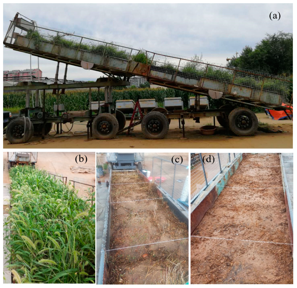
2.1. Experimental Apparatus and Treatments

A variable-slope iron flume 10 m long, 1 m wide, and 0.5 m high was used in the experiment., and the flume is artificially planted with grass strips (Setaria viridis (L.) Beauv.). The flume is shown in Figure 1a. The flume was equipped with water–sediment supply and mixing devices. The experimental sediment was collected from Jixian, Shanxi Province, China. The sediment was typical loess from the Loess Plateau [24], with its physical properties shown in

Table 1. Physical properties of the sediment used in the experiments.

Particle Size Distribution										Soil Type	Soil Texture
Particle size (μm)	>1000	1000–500	500–250	250–100	100–50	50–20	20–2	2–1	<1	Loessial soil	Sandy loam soil
Percentage (%)	0	0.55 ±0.34	1.14 ±0.07	5.27 ±1.48	29.15 ±2.73	46.04 ±1.43	15.32 ±2.15	0.87 ±0.11	1.66 ±0.14

. The grassland has undergone natural flourishing and withering for five years, and its soil surface is eroded little by the experimental flow rate. The experimental treatments were complete grass strips (CG group), remove green grass and retain withered grass (RG group), and remove all green and withered grass (RGW group). The flume was used at a slope of 5° with a flow rate of 30 L min⁻¹ m⁻¹ and a sediment concentration of 120 g L⁻¹. Three repeated experiments were conducted for each treatment group. Photographs of the flume prepared for each experiment group are shown in Figure 1b–d, and the experiment group details are shown in

Table 2. Details of the sediment-trapping experiments using different structural components of the aboveground parts of the grass strips.

Flow Rate (Q)	Sediment Concentration (SC)	Slope	Treatment (Code)	Duration t (min)	Repeated
30 L min−1 m−1	120 g L−1	5°	Completed grass strips (CG)	150	3
			Remove green grass (RG)	120	3
			Remove green and withered grass (RGW)	60	3

. The three independent repeated experiments for each experimental treatment group were labeled 1, 2, and 3, and they were completely corresponding and fixed in this article. Therefore, the experimental codes were CG1, CG2, CG3, RG1, RG2, RG3, RGW1, RGW2, and RGW3, respectively. Based on the results of our previous experimental study [22], the approximate time required to reach a stable state under the various test conditions was estimated, and the estimated duration was extended appropriately for the formal experiments to ensure that the stable state of sediment trapping by the grass strips could be achieved, and the whole process of sediment trapping can be monitored.

The grass strip was sprinkled evenly with water before an experiment was performed until runoff occurred to eliminate differences in soil moisture and infiltration between the different experiments. The flow velocity was measured at five equal intervals and 1 m long sections along the 10 m long grass strip. The flow velocity in each section was measured three times using the dye tracer (KMnO₄) method, and the mean flow velocity was calculated. Several groups of the surface velocity of overland flow were measured intermittently during each experiment. The green and withered grass in the aboveground parts of the experimental grass strips were collected, respectively, dried at 85℃ to constant weight, and then measured the final weight. The weight result was the total amount of organic matter, which is biomass [25]. The biomass values of green and withered grass were 1.170 kg/m² and 0.361 kg/m², respectively, meaning green and withered grass contributed 76.42% and 23.58%, respectively, of the total biomass. Outlet runoff samples were collected at different times during an experiment. Each sample was weighed and then allowed to stand until the supernatant could be removed. The sediment was then dried at 105 °C to a constant weight [20,26]. The results were used to calculate the sediment transport rate at the outflow.

2.2. Measurement and Data Analysis

2.2.1. Sediment Process Calculations

The sediment transport rate Sed(t) (g min⁻¹) was defined as the mass of sediment transported per unit of time. Sed(t) at time t was calculated using the equation [18]

$$Sed\left(t\right)=SC\left(t\right)Q\left(t\right)$$

(2)

where SC(t) and Q(t) are the sediment concentration (g L⁻¹) and flow rate (L min⁻¹), respectively, at time t (min). The ISTE of a grass strip Ie(t) is usually used to indicate the real-time sediment-trapping performance of the grass strip over time [10,11].

$$Ie\left(t\right)=\frac{Se{d}_{in}\left(t\right)-Se{d}_{out}\left(t\right)}{Se{d}_{in}\left(t\right)}=1-\frac{Se{d}_{out}\left(t\right)}{Se{d}_{in}\left(t\right)}$$

(3)

In Equation (3), Sed_in(t) and Sed_out(t) are the inflow and outflow sediment transport rates, respectively. The cumulative amount of sediment trapping R(t) can be calculated as

$$R\left(t\right)={{\displaystyle \sum }}_{i=1}^n\left(Se{d}_{in}\left(t_i\right)-Se{d}_{out}\left(t_i\right)\right)\Delta t_i, (i=1, 2, 3\dots , n),$$

(4)

where i and n indicate the i-th sample and the first n samples, respectively, and Δt_i is the sampling interval for the i-th sample.

2.2.2. Hydraulic Parameters

The overland flow surface velocity V_surf (m s⁻¹) was measured using the KMnO₄ dye tracer method [27], and the mean overland flow velocity V (m s⁻¹) was calculated using the equation

$$V=\mu V_{surf}$$

(5)

where μ is the correction coefficient [28]. The grass strip used in this study belongs to a rough bed surface; thus, μ = 0.75 for transitional or turbulent flow [29].

The Reynolds number (Re) and Froude number (Fr) were calculated using the equations

$$\mathrm{Re}=\frac{VR}{{\nu }_m}$$

(6)

$$\mathrm{Fr}=\frac{V}{\sqrt{gh}}$$

(7)

where R (m) is the hydraulic radius, and h (m) is the mean width of overland flow. g (m s⁻²) is the acceleration caused by gravity, and ν_m (m² s⁻¹) is the kinematic viscosity coefficient of overland flow. h was calculated using the equation

$$h=\frac{Q}{VB}$$

(8)

where Q (m³ s⁻¹) is the flow rate and B (m) is the width of the overland flow.

The Darcy–Weisbach friction factor f and Manning roughness n are often used to describe the resistances of soil bed surfaces and vegetation to the overland flow [30] as follows:

$$f=\frac{8gRS}{V^2}$$

(9)

$$n=\frac{R^{2/3}{S}^{1/2}}{V}$$

(10)

In Equations (9) and (10), g and S are the gravitational acceleration (m s⁻²) and the steepness of the slope (m m⁻¹), respectively.

3. Results and Discussions

3.1. Sediment-Trapping Process

It can be observed from Figure 2 that the sediment transport rate at the outflow first increased and then became stable but that the rate increased markedly differently in the different experiments. The more complete the aboveground grass strip structure was, the longer the system took to reach a stable state (55 min for the CG group, 40 min for the RG group, and 30 min for the RGW group). The sediment transport rate at the outflow for the CG group is shown in Figure 2. It shows that the sediment-trapping efficiency was high for the first ~30 min of the CG group experiments. No clear gentle increase stage occurred at the beginning of the RG group experiments or RGW group experiments (Figure 2). This indicated that only a little amount of sediment was deposited in the early stages of the experiments, the CG group strips had high levels of roughness, the resistance to overland flow was high, and the flow velocity was low.

ISTEs are plotted against time in Figure 3. ISTEs were high in the initial stages of the experiments. For example, ISTEs for the first sampling points in the CG, RG, and RGW group experiments were 0.9950 ± 0.0027, 0.8957 ± 0.0077, and 0.7984 ± 0.0111, respectively. The results indicated that ISTEs were usually higher in the initial stage, and the high ISTEs usually lasted longer for the grass strips with more complete aboveground structures than for the grass strips with less complete aboveground structures. The initial ISTE for the grass strips reached 0.7984 even with the green and withered grass removed. This was still a high ISTE, indicating that soil bed resistance played a major role in the grass strips trapping sediment in the initial stage.

The cumulative amount of sediment trapped R(t) (kg) is plotted against time in Figure 4. R(t) increased rapidly in the early stages of the experiments but increased little in the later stages. The more complete the grass strips were, the faster the rate of R(t) increased in the early stages, and the higher the R(t) was in the stable stages of the experiments. Zhang et al. proposed a formula to calculate the sediment transport capacity of overland flow using slope, flow rate, and median particle size by flat plexiglass bed surface tests [31]. Under our experimental conditions (flow rate 30 L min⁻¹ m⁻¹, median particle size 39.9 μm, slope 5°), the sediment transport capacity of overland flow was ~5620 g min⁻¹, which is greater than the sediment inflow rate in our study (3600 g min⁻¹). Therefore, under the silt-laden inflow conditions (3600 g min⁻¹), the sediment deposition would not occur on a smooth and flat 5° slope bed surface but would occur if the effect of microtopography, gravel particles, and vegetations exist. The bed surface has been covered by some deposited sediment at the stable-state stage in experiments. Although it was not as smooth and flat as the plexiglass bed surface, ISTE fluctuated around 0 (Figure 4), indicating that almost no sediment was deposited in the grass strips during the stable state stage, which also mirrored the findings of Zhang et al. [31]. Sediment deposition in the early stage of the RGW group experiments would therefore have been caused by the microtopography resistances and gravel resistances of the soil bed surface. ISTE also decreased when the soil bed surface was gradually covered by deposited sediment.

R_m (kg) was the total amount of deposited sediment when the stable state stage of sediment trapping was reached. The average and error range of R_m values for the three repeated experiments in CG, RG, and RGW groups were 154.03 ± 5.08 kg, 76.25 ± 3.19 kg, and 46.61 ± 3.52 kg, respectively. The contributions of green grass, withered grass, and the soil bed surface to R_m were therefore 50.50% ± 3.29%, 19.24% ± 2.07%, and 30.26% ± 2.29%, respectively. The green to withered grass biomass ratio was about 3.24:1. The ratio for the green and withered grass contributions to R_m was about 2.62:1. This would mainly have been because some of the withered grass was in a lodging state, whereas the green grass was mostly upright. More sediment would therefore be trapped per unit biomass by the withered grass than the green grass. For the grass strips used in this study, withered grass contributed, per unit biomass, approximately 1.24 times more than green grass to the R_m.

3.2. Overland Flow Regime

Equations (5)–(7) were used to calculate the mean velocity V, Re, and Fr, respectively, for overland flow in the CG, RG, and RGW group experiments, and the ranges of values found are shown in

Table 3. The ranges of the mean velocity (V), Reynolds number (Re), and Froude number (Fr) of overland flow in the different grass strip treatment experiments.

Treatment	Experiment Code	V (m/s)	Re	Fr
Completed grass strips (CG)	CG1	0.047~0.120	508~1016	0.14~0.49
	CG2	0.042~0.116	653~1306	0.09~0.43
	CG3	0.049~0.126	539~1346	0.12~0.49
Remove green grass (RG)	RG1	0.107~0.228	756~2647	0.35~0.69
	RG2	0.097~0.186	802~3474	0.30~0.72
	RG3	0.083~0.185	798~1730	0.24~0.78
Remove green and withered grass (RGW)	RGW1	0.154~0.250	603~1809	0.54~1.19
	RGW2	0.138~0.221	660~1871	0.46~1.02
	RGW3	0.141~0.236	790~2212	0.49~1.22

. Re was >500 for all of the experiments, meaning that overland flow under the experimental conditions we used involved transitional and/or turbulent flow but no laminar flow. The Fr values for most of the experiments were <1, meaning that overland flow was tranquil flow. This may have been because the supercritical flow was hardly to occur at the gentle slope of 5° and the flow rate of 30 L min⁻¹ m⁻¹. Nicosia et al. performed simulated rainfall tests using rainfall intensities between 60 and 181 mm h⁻¹ and slopes of between 3.6% and 39.6% using plots with four different types of vegetation and found Fr values of 0.02–0.47 [32]. This indicated that overland flow was tranquil, similar to the conclusions drawn from the results of our study.

The range of hydraulic parameters cannot indicate the specific differences of the flow regimes in each experimental group. The distributions of V, Re, and Fr in each group were shown in Figure 5. The median ± error overland flow velocity V (m s⁻¹) values for the CG, RG, and RGW group experiments were 0.0951 ± 0.0027, 0.1516 ± 0.0054, and 0.1954 ± 0.0069, respectively. The median lines and box ranges in Figure 5a indicate that the overland flow velocity was higher for the RGW group than the CG group. Resistance caused by withered grass decreased the flow velocity by ~22%, and resistance caused by both green and withered grass decreased the flow velocity by ~51%. The median Re values were slightly lower for the CG group than the RG and RGW groups and were similar for the RG and RGW groups (Figure 5b). Under the influence of deposited sediment, the overland flow regime was constantly changing during the sediment-trapping process. The Fr distributions indicated that most measurement results of the overland flow in each group experiment were tranquil flow. A more complete aboveground part structure caused the flow velocity to be lower and Fr to be lower (Figure 5c). There are some outliers in Figure 5. The outliers of the box plots in this study were identified via the following process. The lower and upper quartiles (D₁ and D₃) are called the 25% and 75% positions of the ascending sequence, respectively. Interquartile range (IQR), D₃ − D₁, is called as the interquartile range in statistics. In a box plot, the data of >D₃ + 3/2 × IQR or <D₁ − 3/2 × IQR are identified as outliers. Outliers are therefore related to the IQR range of the sample sequence, that is, determined by the concentration degree of sample points. The smaller the IQR range is, the more sample points may be identified as outliers.

Removing the green and withered grass caused the Fr for overland flow to occasionally be >1, indicating that the overland flow changed from continuous tranquil flow in the RG and RGW groups to critical and supercritical flow occurring in the CG group. Water was applied evenly to the grassland plots before each experiment until runoff occurred to eliminate differences between the soil moisture contents in the different experiments. No infiltration occurred during the experiments. In one experiment, changes in the overland flow velocity and regime were mainly caused by the sediment deposited during the experiment, which was explained in some previous publications [12,23]. The differences between the overland flow regimes in the different experiments were mainly caused by resistances provided by green grass, withered grass, and the soil surface, which changed the overland flow velocity and regime and finally caused deposition of sediment. It is therefore necessary to investigate resistance to overland flow provided by the aboveground parts of the grass strips.

3.3. Resistances to Overland Flow Provided by the Grass Strips

The mean velocity was calculated from the measured overland flow surface velocity using Equation (5), and the Darcy–Weisbach friction factor f and Manning roughness n were calculated using Equations (9) and (10), respectively. Box plots of the f and n distributions for the different experiments are shown in Figure 6a,b, respectively. There were marked differences between the f and n values for the different experiments. The more the material blocked overland flow on the hillslope, the greater the resistance to overland flow was.

The mean values and error ranges for f and n were 7.26 ± 0.71 and 0.1344 ± 0.0092, respectively, for the CG group; 2.61 ± 0.17 and 0.0773 ± 0.0024, respectively, for the RG group; and 1.10 ± 0.12 and 0.0486 ± 0.0029, respectively, for the RGW group. Removing the green grass decreased the mean f from 7.26 to 2.61, i.e., by 64.05%, and decreased the mean n by 42.49%. Removing the withered grass decreased f by a further 20.80%, to 1.10, and decreased n by a further 21.35%, from 0.0773 to 0.0486. Removing the green grass decreased the total amount of sediment trapped R_m by 50.49%, and removing the withered grass decreased the R_m further by 19.25%. It can be seen that the contributions of the aboveground parts to the total amount of sediment trapped was mainly determined by the resistance of the aboveground parts of the grass strips to overland flow.

Green grass and withered grass increased f by 4.65 and 1.51, respectively, and the ratio between these values was 3.08:1. The green to withered grass biomass ratio was 3.24:1. These two ratios were very similar. It can be seen that the resistance to overland flow provided by green and withered grass was essentially determined by the biomass. Theoretically, the moisture content is markedly higher for green grass than withered grass. If green and withered grass had the same shape, resistance to overland flow would be higher for green grass than withered grass. In fact, f was increased by green and withered grass by 0.397 and 0.418 per kilogram of biomass, respectively, meaning f was increased ~1.05 times more per unit of biomass by withered grass than by green grass. This would mainly have been because the green grass was mostly upright, but the withered grass was mostly lodged or semi-lodged. Resistance to overland flow was therefore increased more by the same biomass of withered grass than of green grass. This was finally reflected in the effect of the green and withered grass on the total amount of sediment trapped by the grass strips.

To date, it is still unclear whether a unified f-S relation exists for granular surfaces or vegetation-covered slopes, or what causes the different f-S relation under shallow overland flow conditions. Inspired by channel or pipe hydraulics, resistance f to overland flow is frequently expressed by the Re as follows: f = K × Re − b, where K and b are regressed parameters. K equals 24 for a smooth surface under a laminar flow regime [33]. It means that slope steepness would have no relation with f because Re is a product of unit flow rate and kinematical viscosity and has nothing with slope [34]. The steeper slopes evolve to rougher surfaces, compared with shallower slopes, and this increase of roughness with slope balanced the increase of flow velocity with slope, resulting in a slope-independent condition [35]. The hypothesis of slope–velocity equilibrium implies that the use of hydraulic equations, such as Manning and Darcy–Weisbach, cannot easily be applied in hillslope scale runoff models [32,36]. Manning and Darcy–Weisbach equations were often used in overland flow studies. In order to compare with the results of previous similar studies, the traditional Manning and Darcy–Weisbach equations were used in this study. However, the use of Manning and Darcy–Weisbach equations for the calculation of the friction factor is limited. The resistance calculation formula of steep hillslope needs to be further improved.

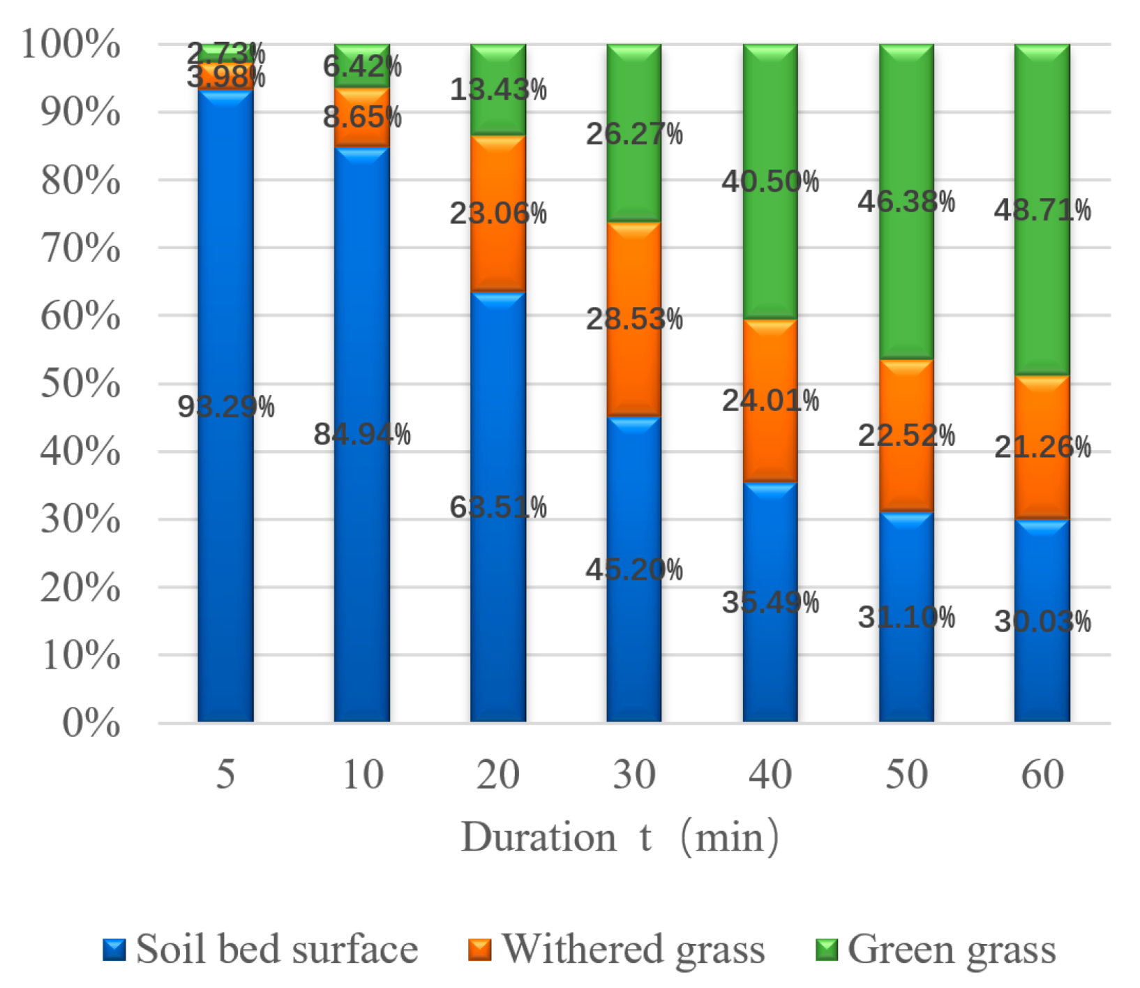
3.4. Temporal Variations in the Contributions of the Aboveground Parts of the Grass Strips to Sediment Trapping

As mentioned above, the ratio of the contributions of green grass, withered grass, and the soil bed surface to the total amount of sediment trapped R_m when the grass strips each reached a stable state were 5:2:3. This ratio was for when the sediment-trapping process reached a stable state so does not reflect the contributions of the aboveground components to sediment trapping in other stages. In reality, rain sometimes falls for a short time, and water and sediment transport over a hillslope will finish before sediment trapping reaches a stable state. It is therefore important to investigate temporal variations in sediment trapping by aboveground grass strip components.

Temporal variations in the cumulative amount of sediment trapped R(t) in the CG, RG, and RGW group experiments are shown in Figure 7. The R(t) curves for the three groups of experiments in the first 10 min were very similar, indicating that the soil bed surface played an important role in the early stage of sediment trapping. After some sediment had been deposited, the R(t) curves for the different treatments continued to increase, and differences in the effects of green grass, withered grass, and the soil bed surface gradually became apparent. As the stable state of the sediment-trapping process for each experimental group gradually was reached, differences between the cumulative amounts of sediment trapped in the different experimental groups became relatively stable after 50 min. The cumulative amounts of sediment trapped at different stages of the different experiments are shown in Table 3.

The vertical bars in, from top to bottom, green, red, and blue, in Figure 8 show the proportions of the cumulative amount of sediment trapped R(t) caused by green grass, withered grass, and the soil bed surface. For example, the fourth bar from the left in Figure 8 indicates the contributions (as percentages) of each aboveground part to the cumulative amount of sediment trapped R(t) in the previous 30 min (i.e., t = 30 min). The lengths of the different colored parts of the bars were different at different times, indicating that the contributions of the different aboveground parts of the grass strips to R(t) changed as the duration of the sediment-trapping process increased. The soil bed surface played a dominant role in the initial stage (the first 5 min) of the sediment-trapping process, contributing ~90% of the sediment trapping that occurred. During the sediment-trapping process, the effect of the soil bed surface became weaker as the deposited sediment coverage increased. Later, the soil bed surface contributed only ~30% of the sediment trapping that occurred in the first 50 min. In addition, the soil bed surface contributed 31.10% of R(t) in the first 50 min and 30.03% of R(t) in the first 60 min, indicating that the soil bed surface had little effect between 50 and 60 min. The contribution of soil bed surface to R(t) was mainly due to the sediment trapped in the first 20 min. Zheng et al. performed a simulated rainfall experiment in a grassland area at the Renjiatai forest farm in Fuxian County, Ziwuling Forest Region, China [37]. The experiment lasted 31 min. The total contribution of stems, branches, and litter to sediment trapping was 44.6% and the contribution of the soil bed to sediment trapping was 55.4%. At 30 min in our study, the contribution of both green and withered grass was 54.8%, and the contribution of the soil bed surface was 45.2%, which were similar to the contributions found by Zheng et al. [37].

As shown in Figure 8, the main factors affecting the cumulative amount of sediment trapped R(t) changed through the sediment-trapping process. The soil bed surface played an important role in the first 30 min, and green grass was dominant after 40 min. Between 5 and 40 min, the contribution of the soil bed surface to R(t) decreased from 93.29% to 35.49%, and the contribution of green grass increased from 2.73% to 40.50%. This indicates that the main structural part contributing to sediment trapping changed from the soil bed surface to green grass. The contribution of withered grass was only 3.98% in the initial stage of sediment trapping but gradually increased to 28.53% at 30 min and then decreased to 21.26% at 60 min. The contribution of withered grass was always between the contributions of green grass and the soil bed surface. The rapid increase in the contribution of green grass and withered grass was mainly caused by the soil bed surface becoming covered with deposited sediment and the resistance of the soil bed surface to overland flow gradually weakening, making the resistance provided by green and withered grass become gradually more prominent. As shown in Figure 7, when sediment trapping occurred for long enough, the contributions of the different components tended to become stable after 50 min. The contributions of the different aboveground parts of the grass strips to R(t) during the sediment-trapping process changed (either increasing or decreasing), but the overall sediment-trapping efficiencies of the grass strips continually decreased until a stable state was reached.

4. Conclusions

The study was mainly focused on the roles of the aboveground parts of grass strips (green grass, withered grass, and the soil bed surface) in the sediment-trapping process and temporal changes during the sediment-trapping process. The main conclusions are shown below.

• The aboveground parts of a grass strip can significantly affect the overland flow regime. The slope of the grass strip used in the experiment was 5°. At a flow rate of 30 L min⁻¹ m⁻¹ and a sediment concentration of 120 g L⁻¹, a continuous and high instantaneous sediment-trapping efficiency segment occurred in the initial stage of the complete grass strip experiments. The results indicated that overland flow in the three treatments involved transitional flow and turbulent flow but not laminar flow. Overland flow in the CG (complete grass strip) and RG (green grass removed) group experiments was always tranquil, but critical and supercritical flow occurred in the RGW (green and withered grass removed) group experiments.
• The resistance factor f increased by 0.397 per kilogram of green grass biomass and by 0.418 per kilogram of withered grass biomass (1.05 times higher than f for green grass). The green and withered grass biomass generally determined the resistance to overland flow. The resistances of the aboveground parts of the grass strips to overland flow effectively determined the contributions of the parts to sediment trapping.
• The soil bed surface played a major role in the initial stage of the sediment-trapping process. As the sediment-trapping process continued, green grass became a more important contributor to sediment trapping. In the initial sediment-trapping stage (the first 5 min), the soil bed surface contributed ~90% of the cumulative amount of sediment trapped R(t). In the stable stage, the contributions of green grass, withered grass, and the soil bed surface to R(t) were ~50%, ~20%, and ~30%, respectively. Therefore, more attention should be paid to the role of soil bed surface if local rainfall occurs mainly for short periods. The layout of grass strips and modification of the microtopography can be combined to increase the sediment-trapping performance. For areas with long-duration rainfall, attention should be paid to improving and maintaining grass coverage so grass strips can effectively trap sediment. The vegetation module in some water–sediment models should be designed to fully consider the effects of different aboveground part compositions in the vegetation area.

These results are helpful to improve the ability to accurately assess the effects of vegetation restoration on sediment transport at the hillslope and watershed scales.

References

1. Hooke, J.; Sandercock, P. Use of vegetation to combat desertification and land degradation: Recommendations and guidelines for spatial strategies in Mediterranean lands. Landsc. Urban Plan. 2012, 107, 389–400. [Google Scholar] [CrossRef]
2. Govers, G.; Rauws, G. Transporting capacity of overland flow on plane and on irregular beds. Earth Surf. Process. Landf. 1986, 11, 515–524. [Google Scholar] [CrossRef]
3. Singhal, M.K.; Mohan, J.; Agrawal, A.K. Role of grain shear stress in sediment transport. Water Energy Int. 1980, 37, 105–108. [Google Scholar]
4. Abrahams, A.D.; Parsons, A.J. Hydraulics of interrill overland flow on stone-covered desert surfaces. Catena 1994, 23, 111–140. [Google Scholar] [CrossRef]
5. Comiti, F.; Cadol, D.; Wohl, E. Flow regimes, bed morphology, and flow resistance in self-formed step-pool channels. Water Resour. Res. 2009, 45, 546–550. [Google Scholar] [CrossRef]
6. Mekonnen, M.; Keesstra, S.; Stroosnijder, L.; Baartman, J.; Maroulis, J. Soil Conservation through Sediment Trapping: A Review. Land Degrad. Dev. 2015, 26, 544–556. [Google Scholar] [CrossRef]
7. Zhou, Z.-C.; Gan, Z.-T.; Shangguan, Z.-P. Sediment Trapping from Hyperconcentrated Flow as Affected by Grass Filter Strips. Pedosphere 2013, 23, 372–375. [Google Scholar] [CrossRef]
8. Nyssen, J.; Clymans, W.; Poesen, J.; Vandecasteele, I.; De Baets, S.; Haregeweyn, N.; Naudts, J.; Hadera, A.; Moeyersons, J.; Haile, M.; et al. How soil conservation affects the catchment sediment budget—A comprehensive study in the north Ethiopian highlands. Earth Surf. Process. Landf. 2009, 34, 1216–1233. [Google Scholar] [CrossRef]
9. Luo, M.; Pan, C.; Liu, C. Modeling study on the time-varying process of sediment trapping in vegetative filter strips. Sci. Total Environ. 2020, 725, 138361. [Google Scholar] [CrossRef]
10. Mekonnen, M.; Keesstra, S.; Ritsema, C.J.; Stroosnijder, L.; Baartman, J. Sediment trapping with indigenous grass species showing differences in plant traits in northwest Ethiopia. Catena 2016, 147, 755–763. [Google Scholar] [CrossRef]
11. Akram, S.; Yu, B.; Ghadiri, H.; Rose, C. Modelling Sediment Trapping by Non-Submerged Grass Buffer Strips Using Nonparametric Supervised Learning Technique. J. Environ. Inform. 2015, 27, 1–13. [Google Scholar] [CrossRef] [Green Version]
12. Farenhorst, A.; Bryan, R. Particle size distribution of sediment transported by shallow flow. Catena 1995, 25, 47–62. [Google Scholar] [CrossRef]
13. Rauws, G. Laboratory experiments on resistance to overland flow due to composite roughness. J. Hydrol. 1988, 103, 37–52. [Google Scholar] [CrossRef]
14. Einstein, H.A.; Banks, R.B. Fluid resistance of composite roughness. Eos Trans. Am. Geophys. Union 1950, 31, 603–610. [Google Scholar] [CrossRef]
15. Weltz, M.A.; Arslan, A.B.; Lane, L.J. Hydraulic Roughness Coefficients for Native Rangelands. J. Irrig. Drain. Eng. 1992, 118, 776–790. [Google Scholar] [CrossRef] [Green Version]
16. Ding, L.; Fu, S.; Liu, B.; Yu, B.; Zhang, G.; Zhao, H. Effects of Pinus tabulaeformis litter cover on the sediment transport capacity of overland flow. Soil Tillage Res. 2020, 204, 104685. [Google Scholar] [CrossRef]
17. Mu, H.; Yu, X.; Fu, S.; Yu, B.; Liu, Y.; Zhang, G. Effect of stem basal cover on the sediment transport capacity of overland flows. Geoderma 2019, 337, 384–393. [Google Scholar] [CrossRef]
18. Jin, C.; Romkens, M.J.M. Experimental Studies of Factors in Determining Sediment Trapping in Vegetative Filter Strips. Trans. ASAE 2001, 44, 277. [Google Scholar] [CrossRef]
19. Loch, R.J. Effects of vegetation cover on runoff and erosion under simulated rain and overland flow on a rehabilitated site on the Meandu Mine, Tarong, Queensland. Soil Res. 2000, 38, 299–312. [Google Scholar] [CrossRef]
20. Wu, T.; Pan, C.; Li, C.; Luo, M.; Wang, X. A field investigation on ephemeral gully erosion processes under different upslope inflow and sediment conditions. J. Hydrol. 2019, 572, 517–527. [Google Scholar] [CrossRef]
21. Nearing, M.A.; Foster, G.R.; Lane, L.J.; Finkner, S.C. A Process-Based Soil Erosion Model for USDA-Water Erosion Prediction Project Technology. Trans. ASAE 1989, 32, 1587–1593. [Google Scholar] [CrossRef]
22. Luo, M.; Pan, C.; Liu, C. Experiments on measuring and verifying sediment trapping capacity of grass strips. Catena 2020, 194, 104714. [Google Scholar] [CrossRef]
23. Luo, M.; Pan, C.; Cui, Y.; Wu, Y.; Liu, C. Sediment particle selectivity and its response to overland flow hydraulics within grass strips. Hydrol. Process. 2020, 34, 5528–5542. [Google Scholar] [CrossRef]
24. Yun, L.; Bi, H.; Gao, L.; Zhu, Q.; Ma, W.; Cui, Z.; Wilcox, B. Soil Moisture and Soil Nutrient Content in Walnut-Crop Intercropping Systems in the Loess Plateau of China. Arid. Land Res. Manag. 2012, 26, 285–296. [Google Scholar] [CrossRef]
25. Mehta, N.; Pandya, N.R.; Thomas, V.O.; Krishnayya, N.S.R. Impact of rainfall gradient on aboveground biomass and soil organic carbon dynamics of forest covers in Gujarat, India. Ecol. Res. 2014, 29, 1053–1063. [Google Scholar] [CrossRef]
26. Saleh, I.; Kavian, A.; Roushan, M.H.; Jafarian, Z. The efficiency of vegetative buffer strips in runoff quality and quantity control. Int. J. Environ. Sci. Technol. 2018, 15, 811–820. [Google Scholar] [CrossRef]
27. Pan, C.; Shangguan, Z. Runoff hydraulic characteristics and sediment generation in sloped grassplots under simulated rainfall conditions. J. Hydrol. 2006, 331, 178–185. [Google Scholar] [CrossRef]
28. Li, G.; Abrahams, A.D.; Atkinson, J.F. Correction Factors in the Determination of Mean Velocity of Overland Flow. Earth Surf. Process. Landf. 1996, 21, 509–515. [Google Scholar] [CrossRef]
29. Luk, S.H.; Merz, W. Use of the salt tracing technique to determine the velocity of overland flow. Soil Technol. 1992, 5, 289–301. [Google Scholar] [CrossRef]
30. Smith, M.; Cox, N.J.; Bracken, L. Applying flow resistance equations to overland flows. Prog. Phys. Geogr. 2007, 31, 363–387. [Google Scholar] [CrossRef]
31. Zhang, G.-H.; Wang, L.-L.; Tang, K.-M.; Luo, R.-T.; Zhang, X.C. Effects of sediment size on transport capacity of overland flow on steep slopes. Hydrol. Sci. J. 2011, 56, 1289–1299. [Google Scholar] [CrossRef]
32. Nicosia, A.; Di Stefano, C.; Pampalone, V.; Palmeri, V.; Ferro, V.; Polyakov, V.; Nearing, M. Testing a theoretical resistance law for overland flow under simulated rainfall with different types of vegetation. Catena 2020, 189, 104482. [Google Scholar] [CrossRef]
33. Emmett, W.W. The Hydraulics of Overland Flow on Hillslopes. 1970. Available online: https://pubs.er.usgs.gov/publication/pp662A (accessed on 6 June 2021). [CrossRef]
34. Pan, C.; Ma, L.; Wainwright, J.; Shangguan, Z. Overland flow resistances on varying slope gradients and partitioning on grassed slopes under simulated rainfall. Water Resour. Res. 2016, 52, 2490–2512. [Google Scholar] [CrossRef] [Green Version]
35. Nearing, M.A.; Polyakov, V.O.; Nichols, M.H.; Hernandez, M.; Li, L.; Zhao, Y.; Armendariz, G. Slope–velocity equilibrium and evolution of surface roughness on a stony hillslope. Hydrol. Earth Syst. Sci. 2017, 21, 3221–3229. [Google Scholar] [CrossRef] [Green Version]
36. Nicosia, A.; Di Stefano, C.; Pampalone, V.; Palmeri, V.; Ferro, V.; Nearing, M.A. Testing a theoretical resistance law for overland flow on a stony hillslope. Hydrol. Process. 2020, 34, 2048–2056. [Google Scholar] [CrossRef]
37. Zheng, F.; Bai, H.; An, S. The benefit analysis for different layers of grass vegetation reducing surface runoff and sediment yield. Res. Soil Water Conserv. 2005, 12, 86–87, 111. [Google Scholar]
Figure 1. Photographs of the experimental setup and the three experimental treatments. (a) Variable-slope iron flume; (b) Completed grass strips; (c) Remove green grass; (d) Remove green and withered grass.
Sustainability 13 07591 g001
Figure 2. Sediment delivery rate at the outlet (Sedout) for the different grass strip treatment experiments.
Sustainability 13 07591 g002
Figure 3. Instantaneous sediment-trapping efficiency plotted against time for the different grass strip treatment experiments.
Sustainability 13 07591 g003
Figure 4. Cumulative amount of sediment trapped plotted against time for the different grass strip treatment experiments.
Sustainability 13 07591 g004
Figure 5. Box plots of (a) the mean flow velocity V, (b) Reynolds number Re, and (c) Froude number Fr data for the different experiments. The red line in the middle of each box is the median. The blue lines below and above the red line indicate the first quartile and third quartile, respectively. The black lines above and below each box are the maximum and minimum values (excluding outliers), respectively. The red plus signs beyond the black horizontal lines are outliers. The vertical length of a blue box is the interquartile range.
Sustainability 13 07591 g005
Figure 6. Box plots of the Darcy–Weisbach resistance factor f and Manning’s roughness n for the grass strip in the different treatment experiments. Note: Some outliers far from the boxes are not shown to improve clarity. The outliers may have been caused by large measurement errors. In plot (a), outliers with f > 30 (eight points) are not shown. These were all found in the complete grass strip experiments. Two of the points were for test CG1, four for testCG2, and two for test CG3. These outlying values were caused by overland flow being much more disturbed in the complete grass strips than in the other strips, making the measurements more unstable for the complete grass strips than the other strips. Outliers with n > 0.3 in plot (b) are not shown and corresponded to the eight outliers for plot (a).
Sustainability 13 07591 g006
Figure 7. Cumulative amount of sediment trapped R(t) plotted against time for the different grass strip treatment experiments. Note: The solid lines indicate the mean values for the repeated experiments, and the upper and lower horizontal lines indicate the upper and lower limits of the measurements.
Sustainability 13 07591 g007
Figure 8. Contributions of the structural components of the aboveground parts of the grass strips to the cumulative amount of sediment trapped over different periods.
Sustainability 13 07591 g008