Article

Do Neighborhoods with Highly Diverse Built Environment Exhibit Different Socio-Economic Profiles as Well? Evidence from Shanghai

1
School of Geography and Planning, Department of Urban and Regional Planning, Sun Yat-sen University, Guangzhou 510275, China
2
Guangdong Key Laboratory for Urbanization and Geo-Simulation, Sun Yat-sen University, Guangzhou 510275, China
*
Author to whom correspondence should be addressed.
Sustainability 2021, 13(14), 7544; https://doi.org/10.3390/su13147544
Submission received: 10 March 2021 / Revised: 29 June 2021 / Accepted: 1 July 2021 / Published: 6 July 2021

Abstract

:
The link between the built environment and residential segregation has long been of interest to the discussion for sustainable and socially resilient cities. However, direct assessments on how extensively diverse built environments affect the social landscapes of cities at the neighborhood level are rare. Here, we investigate whether neighborhoods with a diverse built environment also exhibit different socio-economic profiles. Through a geodemographic approach, we scrutinize the socio-economic composition of Shanghai’s neighborhoods. We statistically compare the top 10% (very high values) to the bottom 10% (very low values) of the following built environment variables: density, land use mix, land use balance, and greenness. We show that high-density areas have three times the percentage of divorced residents than low-density areas. Neighborhoods with a high level of greenness have median values of 30% more residents aged between 25–44 years old and five times the percentage of houses between 60 to 119 m2 than low-greenness areas. In high land-use mix areas, the share of people that live on a pension is 30% more than the low land-use mix areas. The findings of this study can be used to improve the designs of modern, sustainable cities at the neighborhood level, significantly improving quality of life.

1. Introduction

Residential segregation is a spatial phenomenon whereby people are geographically allocated based on their socio-economic status [1]. However, the spatial allocation of residents is affected not only by their income, education, or occupation but also by the built environment [2,3]. The ’built environment’ concept is multi-dimensional. It refers to human-made constructions, from buildings to parks and green spaces to the energy infrastructures, transportation, and communication networks that support and facilitate everyday life. It also includes the aesthetic qualities of a place, from buildings’ interior and exterior designs to landscaping elements, such as trees and their shade [4]. At the neighborhood level, the built environment can be decomposed into four dimensions: (a) density, a metric measuring the activity in a given area (e.g., people per acre, people per job, or ratio of commercial floor space to land area); (b) land use mix, a metric for the proximity of different land uses; (c) street scale, measured as the ratio of building height to street width; and (d) aesthetic qualities, used to measure the attractiveness of a place [4].

1.1. Built Environment Effects on Human Life

The built environment influences many aspects of a person’s life, including accessibility and walkability issues, physical activity levels, physical health quality, well-being, and mental disorders [5,6,7,8,9,10,11]. For example, high-rise housing appears to have negative effects on the psychological well-being of women with young children [12]. Moreover, poor housing quality is also linked to psychological distress [12]. Providing a high land-use mix, especially the integration of residential use with commercial, civic, and recreational uses at the neighborhood level, has become conventional wisdom among urban planners and health professionals [13]. Such a land-use mix allows for a series of activities serving complementary functions to be available in close proximity, motivating residents to walk or bicycle and thus to a more active life [14,15,16,17].
Most studies have sought to identify the associations between socio-economic and health-related indicators and specific built environment variables, such as the link between park access and resident health, land-use mix and walkability, or the health implications of traffic-related air pollution and socio-economic status. For example, Goodman, Wilkinson, Stafford, and Tonne [18] studied how traffic-related air pollution is associated with health problems and identified which socio-economic classes are more susceptible to these effects. Grekousis and Mountrakis [19] studied how increasing developed land use affects socio-economic structure in the conterminous USA. In another study, Xiao, Wang, Li, and Tang [20] conducted spatial clustering on fundamental socio-economic indicators to identify how social inequality was linked to urban park access in Shanghai. Mavoa et al. [21] identified the land-use mix measures that allowed for a better assessment of a walkability index. More recently, Liu et al. [22] studied how neighborhood greenness is linked to mental well-being in Guangzhou, China. Finally, Wang et al. [23] examined how the perceptions of built environment influence health for older Chinese in Beijing, using big data and deep learning.

1.2. Residential Segregation Effects on Human Life

Similarly, residential segregation has been found to affect human health, access to health care, exposure to crime and violence, as well as noxious pollutants and allergens. Segregation has also been associated with increased isolation among individuals and groups, lower levels of inclusion in social clubs, lower civic engagement and access to political power, and increased unemployment rates [24,25]. A considerable body of literature has studied the implications of segregated communities for their residents. For example, Le-Scherban et al. [26] found that African-American patients in segregated communities displayed worse hypertension and diabetes control. Mouw [27] showed that spatial separation between the affluent and poor creates a spatial mismatch between available job positions and job seekers, leading to higher unemployment rates in poor neighborhoods. Finally, segregation has been proved to produce a concentration of poverty [28] and has also been strongly linked to increased crime rates [24].
In China, change in the built environment is often interwoven with residential segregation [29]. Under the rapid urbanization process, peri-urban villages have been gradually surrounded by farmland expropriated for urban development. These areas ultimately transformed into urban villages leading to further expansion of the adjacent urban areas [30]. Meanwhile, villagers have been permitted to keep their housing land and develop their low-density villages into high-density villages, promoting the development of informal rental housing [31]. The buoyance of informal housing has made urban villages become the major settlement of migrants, aggravating the residential segregation level in urban China [30]. Logan [32] has argued that residential segregation might result in environmental injustice affecting the well-being of residents in deprived neighborhoods. For example, externalizing the provision of green space to the private sector and the desire from the wealthier for more private green space are supposed to worsen environmental injustice in urban China [33]. However, Xiao et al. [33] have found that vulnerable population has equitable access to green space due to the planning approach of the government. Except for environmental injustice, residential segregation in urban China has also impeded the process of social integration of migrants, constraining their opportunities for upward social mobility [34,35]. Previous studies have demonstrated that residential segregation and the uneven distribution of public resources in Shanghai have led to disparities in resource availability and accessibility, which ultimately generated inequality in the well-being between locals and migrants [36,37,38].

1.3. Motivation and Contribution: Linking Diverse Built Environment and Neighborhood Socieconomics

Residential segregation and the built environment are interwoven and highly related to physical and mental health and life opportunities. For this reason, understanding how the built environment influences the social landscape of a city is crucial to helping planners improve modern cities [39]. The current literature explores how the built environment affects the ethnic, economic, or other types of residential segregation [1,18,19]. However, little attention has been paid to whether the extreme values (high or low) of built environment variables are associated with different socio-economic profiles. Most studies analyse the main body of data and look at its behavior in terms of means or other statistics. In many cases, however, the extreme values are of more interest. In fact, extreme values analysis can be found in various application domains, such as environment, hydrology, finance, or urban land use [19,40]. The restriction to an analysis of extreme values can be justified since the extreme part of a sample is often of great importance [41]. For example, for the applications mentioned above, such analysis may identify higher concentration of air pollutants, price shocks in related studies, or high rates of developed land consumption [42]. On this account, the statistical insight gained from extremes can be decisive for decision making and policy [19,42].
Focusing on the extreme values in our analysis, allows us to unravel interesting patterns and relations between the built environment variables and socio-economic data that may remain hidden in the complete dataset. Motivated by this concept, we propose a methodological approach that enables us to trace the links between built environment and census variables at a micro-scale. This is the first study to examine if diverse built environments are linked to different socio-economic profiles to the authors’ knowledge. The null hypothesis (Ho) is that there is no statistically significant difference in the median values of a socio-economic variable among neighborhoods having high values in a built-environment variable with neighborhoods having low values in the same built-environment variable. The alternative hypothesis (H1) is that there is a statistically significant difference in the median values of a socio-economic variable among neighborhoods having high values in a built-environment variable with neighborhoods having low values in the same built-environment variable. We used the Mann–Whitney U-test to test this hypothesis.
We propose the following original methodology:
  • We use key built environment factors—such as population density, land-use mix, land-use balance, and neighborhood greenness.
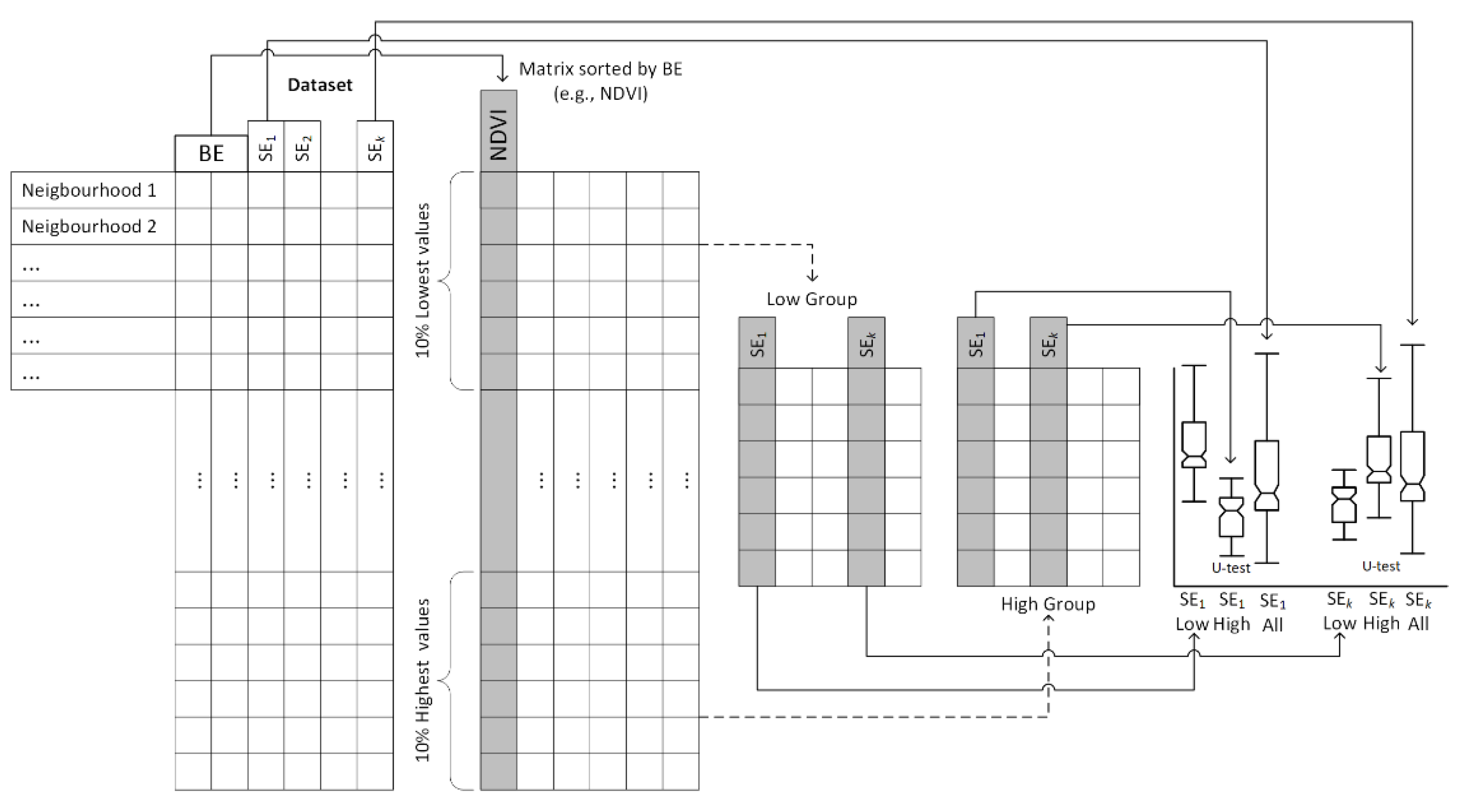
  • Instead of analyzing the entire dataset, as most studies do, we focus only on the 10% higher (90th percentile; high group) and the 10% lower (10th percentile; low group) values of each built environment variable.
  • We cross-compare the socio-economic composition of the low and high groups for each built environment variable. We use 23 variables, reflecting key census dimensions, such s demographic structure, housing, education, source of income, and occupation. Therefore, the analysis of the built environment is conducted through a geodemographic lens.
  • A socio-economic profile is created for each group of values (low and high) for every built environment variable.
  • We use data at the neighborhood level, the finest available scale of analysis for the study area, with an average population of 4000 people per spatial unit. A spatial unit of 4000 people, on average, reflects an aerial size of just a few city blocks, as Shanghai is one of the most densely populated cities (3632 people/km2) in China. In addition, our case study lies in the city center, where population density is even higher (38,171/km2—ten times higher than the average).
  • Using such detailed data allows us to avoid generalizations that might emerge at a lower scale of analysis (e.g., district level) and provides us with many spatial units (n = 2701).
We chose Shanghai for our case study because it is one of the fastest developing and most populated cities in China and worldwide. Shanghai is experiencing increasing social inequality and residential segregation under institutional and market forces (see also the Discussion section) [33,43,44,45]. However, little attention has been paid to the connection between residential segregation and the built environment in Shanghai or urban China in general. As Shanghai faces the challenges of residential segregation [46], it is a paradigmatic illustration of residential segregation in urban China. For this reason, the results of this study can be used to inform policymakers and urban planners of other growing Chinese cities that experience similar challenges. A broader discussion on the socio-economic and historical characteristics of Shanghai as well as how the lessons learned from the Shanghai case study can be helpful in other Chinese cities is provided in the Discussion section. The rest of the paper is organized as follows. Section 2 presents the study’s dataset and methodological approach. Section 3 presents various comparisons through statistical analysis and tests. Finally, Section 4 concludes the paper.

2. Materials and Methods

2.1. Data

Socio-economic information at the neighborhood level was obtained from the Sixth National Population Census of the People’s Republic of China for 2010 [47]. As the smallest unit in urban China, a neighborhood (also referred to as “residential community”) has an average population of 4000 people in Shanghai in 2010, and it is similar to the census tract in the US. Our study area comprises 2701 neighborhoods in the city center of Shanghai, which lies within the Outer Ring Road and includes ten administrative districts: Huangpu, Luwan, Xuhui, Changning, Jing’an, Putuo, Zhabei, Hongkou, Yangpu, and Pudong. In other studies, this area has also been called the “central city” or “main urban metropolitan area” of Shanghai. A total of 23 socio-economic variables are used in this study, covering the main dimensions of the census. For ease of presentation, these have been grouped into five broad domains: age structure, marital status, education, source of income, occupation, and housing (see Table S1).
We also consider the following built environment variables, calculated at the neighborhood level: Density, Land Use Mix, Land Use Balance, and Overall Greenness (see Table S1). Density is the population density, calculated as the number of persons per square kilometer. Land Use Mix is calculated using the entropy index (see Equation (1)). Land Use Balance is calculated using the balance index (see Equation (2)). Land use data were obtained from Shanghai’s Urban and Rural Construction and Transportation Development Institute (http://ghzyj.sh.gov.cn (accessed on 21 November 2020)). The data were collected in 2006 using airborne remote sensing at a 0.4 m × 0.4 m spatial resolution and were classified into nine types following the Classification of Land Use for the City Ecosystem of Shanghai.
Overall greenness is calculated using the Normalized Difference Vegetation Index (NDVI), derived from the Landsat 5 Operational Land Imager and the Thermal Infrared Sensor at a spatial resolution of 30 m. The data covered 2010 and were obtained from USGS EarthExplorer (https://earthexplorer.usgs.gov (accessed on 21 November 2020)); annual averages were used. The NDVI measures the density of greenness in each neighborhood and is used as an aesthetic built-environment variable proxy. The NDVI is a typical remote sensing index and ranges between −1 to 1; higher values indicate healthy and dense vegetation while lower values indicate sparse vegetation [48]; negative values indicate non-biomass areas such as water. The higher the index, the greener the area [2].

2.2. Methods

Instead of analyzing the complete dataset, we focus on built environment variables with extreme values. We rank each built environment variable in turn and we keep the 10% highest (90th percentile) and 10% lowest (10th percentile) values (see Figure 1).
For example, of n = 2701 neighborhoods, we keep the n = 270 corresponding to the spatial units with the 10% lowest NDVI values and the n = 270 neighborhoods with the top 10% NDVI values. Two groups are created: High (e.g., High-NDVI) and Low (e.g., Low-NDVI). We then compare their demographical composition to detect any statistically significant difference in the median values of their variables through the Mann–Whitney median U-statistical test [49]. We also compare each group (High/Low) across the entire study area, including all 2701 neighborhoods, to test whether the High/Low groups are statistically significant different from the full neighborhood group.
More formally, the distributions of each socio-economic characteristic are statistically compared among three groups—Low (<10% rank), High (>90% rank), and all neighborhoods (All) (i.e., High to Low, High to All, and Low to All). A statistically significant difference in socio-economic variables among the three groups indicates that the extreme values of the built environment variable may affect the spatial distribution of the socio-economic variable values tested. However, suppose either the High or Low group is not statistically significant different from the All group. In that case, we will not determine a difference between the High–Low groups (even if the p-value is small), as one of those will be similar to the All group. In that case, the results are interpreted based on the distribution of values for the entire set of neighborhoods.
Various measures have been proposed to quantify land-use mix, from the share of total land area per land-use type to land use mix diversity and dissimilarity indices such as the Balance Index, the Entropy Index, the Atkinson Index, and the Gini Index. (For a complete review, refer to Song et al. [13].) We used two indices: the entropy index and the balance index. These are explained below.

2.2.1. Entropy Index

The entropy index [50] is defined in Equation (1):
LUM = −[p1*ln(p1) + p2*ln(p2) +…+ pi*ln(pi)+…+pn*ln(pn)]/ln(n)
where LUM is the land-use mix score, pi is the proportion of the spatial unit covered by land use i against all land-use categories present in the spatial unit, and n is the number of land use categories.
A LUM score of 1 indicates the maximum possible mix (in which all land-use types are equally present), while a LUM score of 0 indicates the presence of a single land-use for the entire spatial unit.
The LUM formula can be modified to include only the specific categories relevant to the study carried out each time [21]. This study uses nine land-use categories for 2006: Industrial Land, Transportation Land, Public Building Land, Residential Land, Green Land (excluding forests), Municipality Utility Land, Agricultural Land, Water, and Other. Our goal is to assign high rankings to neighborhoods with high mix values for land-use categories that promote quality of life (e.g., walkability). For example, mixing industrial land with residential land is not beneficial to human health. Therefore, we calculate the Revised Entropy Index (REI) using the same formula as in the original LUM (1) considering only the following categories: Residential Land, Green Land (excluding forests), and Public Building Land [15]. The higher the REI value, the more mixed the three land-use categories are. This is generally seen to promote human health, as it reflects a closer integration of residential development with civic and recreational uses [13]. On the other hand, the smaller the REI value, the lower the land-use mix, which is not preferred.

2.2.2. Balance Index

The balance index measures the level to which two different land-use types are balanced in the study area. The index ranges from 0 to 1. Values close to 1 are more balanced. The lower the index value, the less balanced the two land-use types are; this indicates that one type dominates in terms of percentage coverage. It is calculated as shown in Equation (2):
BAL = 1 − |X − aY|/(X + aY)
where,
  • X is the percentage coverage of the first land-use type,
  • Y is the percentage coverage of the second land-use type, and a is a coefficient calculated as a = X*⁄Y* used to adjust the relative balance of X* and Y* within the entire study area; this is used as a benchmark for an acceptable level of balance.
Equation (2) is established to compare only two land-use types, but it can be modified to include a larger number [13].
We group the nine available land-use types into two categories: “desired” and “undesired.” The desired category includes Transportation, Residential Land, Green Land, and Public Building Land. The undesired category comprises the rest of the land-use types: Industrial Land, Municipality Utility Land, Agricultural Land, Water, and Other. The undesired land-use types do not promote interactions or walkability for residents and may harm their health. For example, having industrial use mixed with residential use is not desired. Similarly, having livestock and poultry farms (agricultural land-use types) mixed with residential use or having waste treatment plants and garbage dumps next to residences is also not desired. We calculate the balance index between the desired land-use category (the sum of all percentages in this category) and the undesired land-use category (the sum of all percentages in this category). A high balance index value indicates that the desired and undesired land uses are nearly equally present in the same neighborhood, which is not preferred. The lower the balance, the better separated these two categories are.

3. Results

This section presents the analysis results for each built environment variable over the 23 socio-economic variables. As the analysis is quite extensive, we comment only on the key findings that are statistically significant. We present the socio-economic variables’ median values graphically (see Figure 2A). We also include the p-values across the three comparison groups (i.e., High to Low, Low to High, All to High) (see Figure 2B). This depiction allows for comparing the socio-economic profiles of each subgroup and the tracing of their differences quickly and efficiently.

3.1. NDVI

The results for NDVI are presented in Tables S2 and S3, Figure 2, Figure 3 and Figure 4.
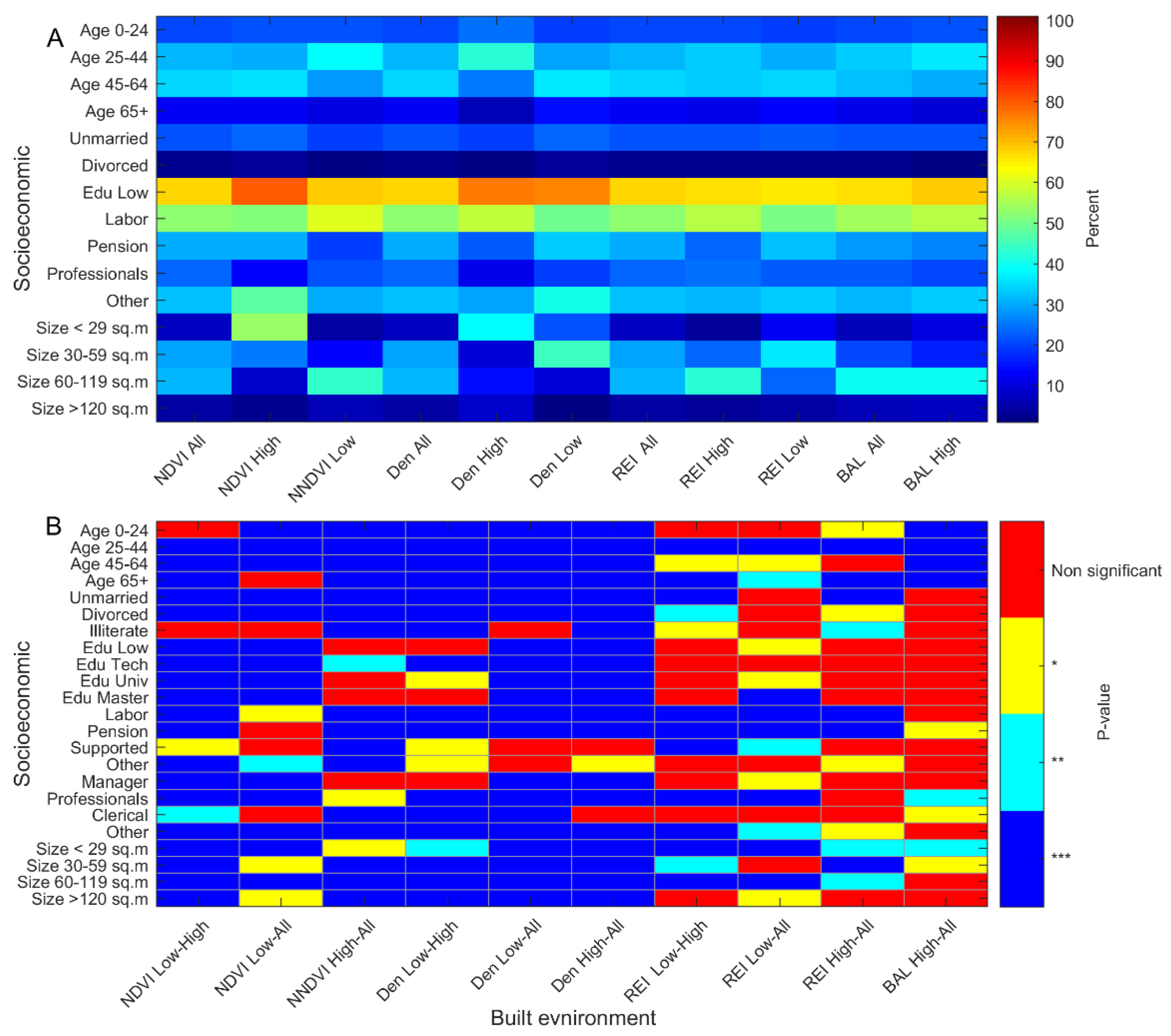
  • Age: High-NDVI areas have statistically significant differences with the Low-NDVI and All groups (see Table S3, Figure 2 and Figure 3). On median values, they have more people (38.80%) between 25 and 44 than the Low-NDVI (30.35%) and the All (31.53%) groups have (see Table S2). They also have fewer people between 45 and 64 (28.94%) than the All group (34.16%) and fewer people 65 years or more (10.15%) than the All group (12.65%). On the other hand, the Low-NDVI areas have more people between 45 and 64 (35.42%) than the High-NDVI areas (28.94%).
  • Marital status: The High-NDVI areas have statistically significant differences with Low-NDVI areas and the All group in both the “Unmarried” and “Divorced” variables (see Table S3, Figure 2 and Figure 3). The High-NDVI areas have lower median values of unmarried people (19.47%) than the Low-NDVI areas (23.04%) (see Table S2). The median divorced people value in the High-NDVI areas is 1.68%, almost half that (3.17%) of the Low-NDVI areas.
  • Education: The High NDVI, Low NDVI, and All groups have no statistically significant differences in illiteracy (see Table S3). The Low-NDVI areas have statistically significant differences in “Lower education” compared to the All group (see Table S3, Figure 2 and Figure 3). In the Low-NDVI areas, 79.08% of people have lower education compared to the 67.08% in All areas (median values; see Table S2). The Low-NDVI areas have the smallest shares of people with a bachelor’s or master’s degree.
  • Source of income: High-NDVI neighborhoods have statistically significant differences in “Income from labor” with both the Low-NDVI and All groups (see Table S3, Figure 2 and Figure 3). The median share of people who receive their main income from labor in the High-NDVI areas is 60.98%; in the Low-NDVI areas, this figure is 51.47% (see Table S2). On the other hand, the High-NDVI areas have fewer people who receive their main income from pensions (19.54%) than the All group (30.00%).
  • Occupation: The High-NDVI neighborhoods have statistically significant differences with the Low-NDVI areas in all occupation variables (see Table S3, Figure 2 and Figure 3). The most striking difference is in the “Other” category, where the Low-NDVI areas have a median value of 47.10%, 50% more than that of the High-NDVI areas (30.32%) (see Table S2). The High-NDVI areas and All areas have similar manager shares (6.82% vs. 6.67%), so we cannot conclude that High NDVI affects this variable. However, the Low-NDVI areas have considerably fewer managers (3.54%). The three groups seem to have equal numbers of people working as office clerks.
  • Housing: The High-NDVI neighborhoods have statistically significant differences with the Low-NDVI areas and All neighborhoods in all house-size variables (see Table S3, Figure 2 and Figure 3). The neighborhoods with High-NDVI values have, based on median values, larger houses than neighborhoods with Low-NDVI values. For example, small houses (less than 29 m2) account for 53.68% of the houses in the Low-NDVI areas and 4.15% in the High-NDVI areas (see Table S2). On the other hand, medium-to-large houses (60 to 119 m2) predominate in the High-NDVI areas (43.52%, median); in the Low-NDVI areas, the median value is 8.65%.

3.2. Density

Results for Density are presented in Tables S3 and S4, Figure 1 and Figure 4, and Figure S1.
  • Age: The low-density areas have significantly larger shares of people between 25 and 44 (42.52%) and 0 and 24 (24.20%) than the High-density areas (29.22% and 19.45%, respectively) (see Tables S3 and S4, Figure S1). On the other hand, the High-density areas have larger shares of those over 45. For example, in the High-density areas, 14.91% of residents are over 65, on average, while this figure is only 7.25% in the Low-density areas (see Table S4).
  • Marital status: The High-density areas have three times the share of divorced residents (3.36%) than the Low-density areas have (1.18%) (see Table S4).
  • Education: Only the “Tech” variable shows statistically significant differences across all three groups (see Table S3).
  • Source of income: The High-density neighborhoods have statistically significant differences in “Income from labor” and “Income from pension” with both the Low-density and All groups (see Table S3, Figure 2 and Figure S1). The median share of people receiving their main income from labor is 49.77% in the High-density areas and 57.91% in the Low-density areas (see Table S4). On the other hand, the Low-density areas have fewer people receiving their main income from pensions (22.78%) than the High-density areas (33.20%).
  • Occupation: The Low-density neighborhoods have statistically significant differences with the High-density areas in “Professionals” and “Other” workers (see Table S3, Figure 2 and Figure S1). The High-density areas have larger shares in “Other” (40.19%) and “Professionals” (19.00%) than the Low-density areas (29.18% and 11.69%, respectively) (see Table S4).
  • Housing: The Low-density neighborhoods have statistically significant differences with the High-density areas and All neighborhoods in all house size variables (see Table S3, Figure 2 and Figure S1). The Neighborhoods with High-density values have, based on median values, smaller houses than the neighborhoods with Low-density values. For example, the median value for houses between 30 and 59 m2 is 44.64% in the High-density areas and 9.20% in the Low-NDVI areas (see Table S4). On the other hand, very large houses (120+ m2) predominate in the Low-NDVI areas, with a median value of 8.16%, while the High-density areas have a median value of 0.95% (almost one-eighth).

3.3. REI

Results for REI are presented in Tables S3 and S5, Figure 2 and Figure 4, and Figure S2.
  • Age: The High-REI areas have statistically significant differences with the Low-REI and All groups only in the 25–44 and 65+ age groups (see Table S3, and Figure S2). The neighborhoods with a low land-use mix have more residents aged 25 to 44 than the neighborhoods with a high land-use mix have (see Table S5). By contrast, the neighborhoods with a high land-use mix have more residents 65 or older.
  • Source of income: The High-REI neighborhoods have statistically significant differences in “Income from labor” with both the Low-REI and All groups (see Table S3, Figure 2 and Figure S2). The median share of people receiving their primary income from labor is 50.36% in the High-REI areas and 56.14% in the Low-REI areas (see Table S5). On the other hand, the High-REI areas have more people receiving their main income from pensions (32.10%) than the Low-REI areas have (23.60%).
  • Housing: The High-REI neighborhoods have statistically significant differences with the Low-REI areas in small houses (less than 29 m2) and medium-sized houses (60 to 119 m2 (see Table S3 and Figure S2). The share of small houses is 12.97% in the High-REI-areas but only 3.51% in the Low-REI areas (see Table S5). On the other hand, the Low-REI areas have, based on median values, more houses in the 60–119 m2 range (42.60%) than the High-REI neighborhoods have (24.00%).

3.4. BAL

The results for BAL are presented in Tables S3 and S6, Figure 2 and Figure 4, Figure S2. The results for BAL are presented in Tables S3 and S6, Figure 2 and Figure 4, and Figure S2.
  • Age: The High-BAL areas have significantly higher shares in (36.10%) between 25 and 44 than the All group (33.97%; see Tables S3 and S6, Figure 2 and Figure S2). They also have lower shares for people between 45 and 64 and 65 or older than the All group.
  • Housing: The High-BAL neighborhoods have statistically significant differences with the All group areas in small houses (less than 29 m2) and small-to-medium-sized houses (30 to 59 m2; see Tables S3 and S6, Figure S2). The share of small houses is 10.86% in the High-BAL areas and only 6.58% in All areas (see Table S6). On the other hand, the High-BAL areas have, based on median values, fewer houses in the 30–59 m2 range (16.91%) than All neighborhoods (20.72%).
We also test whether these groups consist of different neighborhoods. For example, if the High-density and the Low-NDVI groups contain the same spatial entities, we cannot trace which variable is associated with the socio-economic variables studied. In this case, Low-NDVI and High-density are strongly correlated. On the other hand, if the groups consist of different neighborhoods, we cannot apply a correlation analysis due to the lack of a one-to-one linkage between a neighborhood belonging to the one set and a neighborhood belonging to the other. To check for group overlap, we calculate the percentage of common neighborhoods between (a) High-density and High-NDVI, (b) High-density and Low-NDVI, (c) Low-density and High-NDVI, and (d) Low-density and Low-NDVI, as well as the reverse linkages (see Table S7). The higher the percentage, the larger the number of neighborhoods belonging to both sets; the smaller the percentage, the more independent the sets are. The highest percentage is between the Low-density and High-NDVI pair. It is not very high, however, and we can regard all groups as being different.

4. Discussion and Conclusions

Dealing with the legacy of its past, Shanghai has experienced severe socio-spatial segregation throughout its recent history [51]. The urban space of pre-1949 Shanghai was differentiated into an ‘upper-end,’ (containing the French Concession and the International Settlement), and the ‘lower-end,’ (containing the shantytowns built by rural migrants) [52]. During the period of the planned economy (1949–1979), Shanghai’s segregation lessened due to the stringent household registration (hukou) system and the state-dominated allocation of public services and resources. The household registration system was the primary tool used to control internal migration. However, this policy excluded rural residents from urban public goods and services [53,54]. In urban areas, the government monopolized public resources such as housing, education, and health care through state-owned work units [43]. Shanghai residents without local hukou could hardly find a job in the state-owned work units, let alone obtain access to the associated public services and resources. Thus, institutional forces played the leading role in shaping the socio-spatial structure of Shanghai, and Shanghai experienced a low degree of segregation in the planned economy period.
Since China’s reform and opening began in the late 1970s, the influx of rural migrants and the impact of marketization have exacerbated residential segregation in Shanghai. Wu and Li [43] found several dimensions of segregation in urban China relating to human capital (such as education), position in the economic structure (such as occupation and employment status), and institutional constraints (such as hukou status). However, these dimensions are not consistent with the three dimensions proposed by Shevky and Bell [55] in the Western context. Based on the fifth decennial census in 2000, a large body of research has demonstrated that segregation based on hukou status and housing tenure were prominent in Shanghai. However, segregation based on socio-economic status such as education and employment was not evident or severe in the first two decades after reforms began [43,44,56,57,58]. Li and Wu [44] indicated that tenure-based segregation in Shanghai became severer than other dimensions, such as hukou status and education. This can be attributed to the fact that housing tenure represented a pre-existing institutional privilege and a capitalized privilege flowing from the reform. The boom in migrant enclaves and gated communities has gradually reconstructed the socio-spatial structure in Shanghai [59]. Under the joint influences of the path-dependency of the socialist era, rural-to-urban migration, and economic reform, the trend toward segregation via socio-economic status has become much more apparent over recent years [56,60]. Recent research based on the sixth decennial census of Shanghai in 2010 has revealed that education segregation has exceeded the level of hukou segregation, and that Shanghai has become more heavily partitioned based on individual socio-economic status [60]. Segregation based on hukou status and socio-economic status such as occupation and education coexisted and deepened from 2000 to 2010 [61,62]. Meanwhile, the active regulation and redevelopment projects of Shanghai’s municipal government have, along with suburbanization, shaped the city’s center and periphery in several ways, redistributing the city’s population according to socio-economic status [63,64]. The disadvantaged have been stuck in suburban areas and suffer from unequal access to public services and resources, which has undermined their social mobility and deprived them of their rights to public goods [34,35,45]. Much of what is described above is supported by our findings, which also include the built environment dimension and are further discussed below and summarized in Table 1.
Most High-NDVI areas are located outside the city’s core and consist of more younger residents than Low-NDVI areas based on the median values (see Figure 4). The Low-NDVI areas are located at the city’s center and have older people (45–64 and 65+). The High-NDVI areas have more spacious houses than the Low-NDVI areas. The differences are extreme, especially in terms of medium-to-large houses. The High-NDVI areas have, based on median values, five times the share of houses between 60 and 119 m2 (43.52%) that the Low-NDVI areas have (8.65%). The High-NDVI areas have three times the percentage of large houses, those over 120 m2 (6.78%), that the low-NDVI areas have (2.83%) and 50% more than All neighborhoods have (4.33%). We focus on the city center of Shanghai, and the presence of larger houses in greener areas cannot be explained simply by pointing out that these neighborhoods are in the suburbs, where houses are expected to be larger and the natural environment richer. The Low-NDVI areas have higher percentages of unmarried and divorced people than the High-NDVI areas; this might also explain their preference for smaller houses.
The Low-NDVI areas have the lowest percentages of people with a bachelor’s or master’s degree, which is in accordance with previous findings [44]. The High-NDVI areas have no differences from the All group, indicating that, although extremely low NDVI values may affect the educational attainment distribution, extremely high NDVI values do not.
In the High-NDVI areas, the percentage of people that earn their mean income from labor is 20% more than in the Low-NDVI areas. Similarly, the percentage of people that live on pensions is 30% less than in the All group. The fact that more High-NDVI residents gain their income from labor may explain why they can afford to stay in larger houses, because income from labor is significantly higher than that from pensions. In addition, income from labor implies younger people and larger families. On the other hand, income from pensions indicates advanced age and a household of typically one or two members. Finally, the Low-NDVI areas have the highest share of people in skilled occupations, technicians, and workers in commerce and service sectors (‘Other’ category; 50% more than the corresponding share in the High-NDVI areas) and half the share of managers (3.54%) than that of the All group. This may be attributed to the abundant employment opportunities in middle- and low-end service industry and the convenient residential location in the city center [62].
Low-density areas are located outside the city core (see Figure 4). They have an average of 50% more people aged 25 to 44 than High-density areas. The emergency of migrant neighborhoods in the outskirts of the city center might contribute to this [60]. Additionally, in large Chinese cities such as Shanghai, migrants have a younger age structure than the local residents [35]. On the other hand, on average, the High-density areas have nearly double the share of the population over 65 than the Low-density areas. High-density areas are mainly located in the center of Shanghai. The share of divorced people in Low-density areas is under a third of the share in High-density areas. This difference may occur because the High-density areas have higher shares of older people, which increases the number of divorced people. Generally, there are no educational differences between the High- and Low-density areas. In the Low-density areas, the percentage of people that earn their mean income from labor is 20% more than the High-density areas. The share of people living on pensions is 30% less than in the High-density areas. The higher shares of laboring people in the Low-density areas can be partially attributed to the fact that more migrants reside there, most of whom live in Shanghai without social insurance (e.g., unemployment insurance, work injury insurance) [65]. High-density areas have more professionals than Low-density areas, while Low-density areas have more spacious houses than High-density areas. The differences are especially evident regarding medium-sized houses (30–59 m2), of which High-density areas have, on average, four times the share that Low-density areas have (44.46% vs. 9.2%). Low-density areas have eight times the share of large houses (those over 120 m2), based on median values, that High-density areas have a 50% increased share than the All neighborhoods group has. Most of the Low-density areas are located in the outskirts of the city center and were developed in the last two decades. Since the housing marketization in the 2000s, real estate enterprises were involved in the development of commodity housing and larger houses were constructed for the increasing residential needs of the new-rich class [44].
High-land-use mix neighborhoods have, on average, more people aged 65 or older than low land-use mix neighborhoods, which have more people between 25 and 44. The share of people living on pensions is 30% less than in High land use mix areas compared to Low-land-use mix areas. The High-land use mix neighborhoods highly concentrate in the southeast of the city center, where the major government agencies, academic institutions and universities of Shanghai are located [44]. With house ownership acquired in the 1990s, people who retired from these agencies still reside in the original work unit communities. Low-land-use mix areas, mostly fallen into the newly built commodity housing communities, also have more spacious houses.
This research studies how the built environment shapes Shanghai’s social landscape. As Shanghai is the most populated city in the country, it can be considered a paradigmatic illustration of residential segregation in urban China. Therefore, the lessons learned from the Shanghai case study can be helpful in other fast-growing cities in the country. In fact, China has become the world’s largest and most rapidly transforming urban society [66]. With more than 800 million urban residents in 2018 and another 30 million added every year [67], urban China could top 1 billion people in the next decade. By 2030, China is expected to have eight cities with more than 10 million and 19 cities with 5 to 10 million people [67]. As a consequence of the ongoing urbanization trend, China faces multiple sustainable development challenges, including residential segregation [68].
The need for a sustainable and people-centered approach as a guiding principle for urbanization is acknowledged in the National New-type Urbanization Plan released in 2014 by the Chinese government [68]. Therefore, the findings of this study could assist policymakers and urban planners in addressing residential segregation in other Chinese cities. For example, we showed that neighborhood greenness levels seem to affect the social landscape of neighborhoods. In this sense, designing city expansions should prioritize high levels of greenery, something that is also linked to physical and mental health [11]. We also showed that areas with a low land-use mix have different socio-economic characteristics than high land-use mix areas. As other studies have shown, a mixed land-use neighborhood motivates its residents to walk (or bicycle) and fosters more active lifestyles, which in turn promotes physical and mental health [15]. For example, the risk of obesity increases as the land-use mix declines [16,17]. For this reason, planning should consider a closer integration of residential development with civic and recreational uses, something that has been supported by other studies as well [13]. Land-use mix is not always desirable, however. Mixing industrial and residential uses may affect residents’ health or housing values. In this sense, land use mix balance should be considered in sustainable city planning. This research showed that neighborhoods with a high balance index (i.e., residential use is mixed with industrial use) have younger residents (25–44 years old) living in small houses (<29 m2). This can be attributed to the fact that many young people cannot afford to live in larger houses or houses of similar size located in neighborhoods with a lower presence of undesired land uses (i.e., industrial or agricultural land). In this sense, a separation between desired and undesired land uses (in terms of residential living) should be promoted.
In general, improving the built environment of the deteriorating neighborhoods and promoting social mix policies are necessary to mitigate residential segregation in urban China. As the gated community becomes dominant in the real estate market [69], disparities in the residential environment between the old neighborhoods and the newly-built gated communities have led to a higher level of residential segregation [33,36]. Therefore, the government is advised to increase the quantity and quality of public open space such as green spaces, esplanades, and recreational facilities and promote the redevelopment of the deteriorating neighborhoods. Furthermore, application for public housing is skewed towards local residents with low-income and low-income migrants with stable jobs [65]. Migrants excluded from such civic entitlement tend to concentrate on informal housing in urban villages [34,60]. Relaxing the eligibility criteria for public housing can grant more people access to decent housing, mitigating residential segregation in urban villages. Additionally, the government is advised to provide public housing in middle-class neighborhoods for the development of mixed communities. Exposure to a higher class can promote the social integration of the disadvantaged and lower residential segregation levels in urban China
Owing to the limitation of the availability of the latest data (when this paper was written, data of the Seventh Population Census of the People’s Republic of China conducted in 2020 was not available), this article failed to depict the latest socio-economic profile of Shanghai. However, the proposed methodology can be replicated for data retrieved from upcoming censuses and be used in comparative studies. For example, planned future research will integrate socio-economic variables obtained from the Seventh Population Census (2020). Updated vegetation and land use data referring to 2020 will also be included. Comparisons between the 2010 results of this study and the 2020 data will be conducted to provide better insights into neighborhood socio-economic dynamics. In conclusion, policymakers and planners can use the findings of this and similar studies to design modern sustainable cities and significantly improve the quality of life at the neighborhood level.

Supplementary Materials

The following are available online at https://www.mdpi.com/article/10.3390/su13147544/s1, Table S1: Socio-economic and built environment variables used in this study; Table S2: NDVI summary statistics (75th percentile, median, mean, 25th percentile, standard deviation) per variable and group; Table S3: p-values for all comparisons; Table S4: Density summary statistics (75th percentile, median, mean, 25th percentile, standard deviation) per variable and group; Table S5: REI summary statistics (75th percentile, median, mean, 25th percentile, standard deviation) per variable and group; Table S6: BAL summary statistics (75th percentile, median, mean, 25th percentile, standard deviation) per variable and group; Table S7: Percentage of common neighborhoods in groups; Figure S1: Distributions of Low (L) and High (H) density groups as well as the complete set (A) across age, marital status, education, source of income, occupation, and housing; Figure S2: Distributions of Low (L) and High (H) REI and BAL groups as well as the complete set (A) across age, source of income, and housing.

Author Contributions

Conceptualization, G.G.; methodology, G.G.; software, G.G. and Z.P.; writing—original draft preparation, G.G. and Z.P.; writing—review and editing, G.G. and Y.L.; visualization, G.G. and Z.P.; funding acquisition, Y.L. All authors have read and agreed to the published version of the manuscript.

Funding

This research was funded by Fundamental Research Funds for the Central Universities (No. 20lgzd10), and the National Natural Science Foundation of China, grant number 41871140.

Institutional Review Board Statement

Not applicable.

Data Availability Statement

The datasets used and/or analyzed during the current study are available from the corresponding author on reasonable request.

Acknowledgments

Data analyzed in this paper were obtained from the Sixth National Population Census of the People’ Republic of China for 2010. The views expressed herein are the authors.

Conflicts of Interest

The authors declare no conflict of interest.

References

  1. Spielman, S.E.; Harrison, P. The Co-Evolution of Residential Segregation and the Built Environment at the Turn of the 20th Century: A Schelling model. Trans. GIS 2014, 18, 25–45. [Google Scholar] [CrossRef] [Green Version]
  2. Wang, R.; Helbich, M.; Yao, Y.; Zhang, J.; Liu, P.; Yuan, Y.; Liu, Y. Urban Greenery and Mental Wellbeing in Adults: Cross-Sectional Mediation Analyses on Multiple Pathways across Different Greenery Measures. Environ. Res. 2019, 176, 108535. [Google Scholar] [CrossRef] [Green Version]
  3. Grekousis, G. Local Fuzzy Geographically Weighted Clustering: A New Method for Geodemographic Segmentation. Int. J. Geogr. Inf. Sci. 2021, 35, 152–174. [Google Scholar] [CrossRef]
  4. Handy, S.; Boarnet, M.G.; Ewing, R.; Killingsworth, R.E. How the Built Environment Affects Physical Activity: Views from Urban Planning. Am. J. Prev. Med. 2002, 23, 64–73. [Google Scholar] [CrossRef]
  5. Roof, K.; Oleru, N. Public Health: Seattle and King County’s Push for the Built Environment. J. Environ. Health 2008, 71, 24–27. [Google Scholar]
  6. Assari, A.; Birashk, B.; Mousavinik, M.; Naghdbishi, R. Impact of Built Environment on Mental Health: Review of Tehran City in Iran. Int. J. Tech. Phys. Probl. Eng. 2016, 8, 81–87. [Google Scholar]
  7. Grekousis, G.; Mountrakis, G.; Kavouras, M. Linking MODIS-Derived Forest and Cropland Land Cover 2011 Estimations to Socio-Economic and Environmental Indicators for the European Union’s 28 Countries. Gisci. Remote. Sens. 2016, 53, 122–146. [Google Scholar] [CrossRef]
  8. Sander, H.A.; Ghosh, D.; Hodson, C.B. Varying Age-Gender Associations between Body Mass Index and Urban Greenspace. Urban For. Urban Green. 2017, 26, 1–10. [Google Scholar] [CrossRef]
  9. Wu, J.; Rappazzo, K.M.; Simpson, R.J., Jr.; Joodi, G.; Pursell, I.W.; Mounsey, J.P.; Cascio, W.E.; Jackson, L.E. Exploring Links between Greenspace and Sudden Unexpected Death: A Spatial Analysis. Environ. Int. 2018, 113, 114–121. [Google Scholar] [CrossRef] [PubMed]
  10. Hunter, R.F.; Cleland, C.; Cleary, A.; Droomers, M.; Wheeler, B.W.; Sinnett, D.; Nieuwenhuijsen, M.J.; Braubach, M. Environmental, Health, Wellbeing, Social and Equity Effects of Urban Green Space Interventions: A Meta-Narrative Evidence Synthesis. Environ. Int. 2019, 130, 104923. [Google Scholar] [CrossRef]
  11. Huang, B.; Xiao, T.; Grekousis, G.; Zhao, H.; He, J.; Dong, G.; Liu, Y. Greenness-Air Pollution-Physical Activity-Hypertension Association among Middle-Aged and Older Adults: Evidence from Urban and Rural China. Environ. Res. 2021, 195, 110836. [Google Scholar] [CrossRef] [PubMed]
  12. Evans, G.W. The Built Environment and Mental Health. J. Urban Health 2003, 80, 536–555. [Google Scholar] [CrossRef] [PubMed]
  13. Song, Y.; Merlin, L.; Rodriguez, D. Comparing Measures of Urban Land Use Mix. Comput. Environ. Urban. 2013, 42, 1–13. [Google Scholar] [CrossRef]
  14. Tian, L.; Liang, Y.; Zhang, B. Measuring Residential and Industrial Land Use Mix in the Peri-Urban Areas of China. Land Use Policy 2017, 69, 427–438. [Google Scholar] [CrossRef]
  15. Duncan, M.J.; Winkler, E.; Sugiyama, T.; Cerin, E.; duToit, L.; Leslie, E.; Owen, N. Relationships of Land Use Mix with Walking for Transport: Do Land Uses and Geographical Scale Matter? J. Urban Health 2010, 87, 782–795. [Google Scholar] [CrossRef] [Green Version]
  16. Xu, Y.; Wang, L.; Fu, C.; Kosmyna, T. A Fishnet-Constrained Land Use Mix Index Derived from Remotely Sensed Data. Ann. GIS 2017, 23, 303–313. [Google Scholar] [CrossRef] [Green Version]
  17. Manaugh, K.; Kreider, T. What Is Mixed Use? Presenting an Interaction Method for Measuring Land Use Mix. J. Transp. Land Use 2013, 6, 63–72. [Google Scholar] [CrossRef]
  18. Goodman, A.; Wilkinson, P.; Stafford, M.; Tonne, C. Characterising Socio-Economic Inequalities in Exposure to Air Pollution: A Comparison of Socio-Economic Markers and Scales of Measurement. Health Place 2011, 17, 767–774. [Google Scholar] [CrossRef] [Green Version]
  19. Grekousis, G.; Mountrakis, G. Sustainable Development under Population Pressure: Lessons from Developed Land Consumption in the Conterminous US. PLoS ONE 2015, 10, e0119675. [Google Scholar] [CrossRef]
  20. Xiao, Y.; Wang, Z.; Li, Z.; Tang, Z. An Assessment of Urban Park Access in Shanghai–Implications for the Social Equity in Urban China. Landsc. Urban. Plan. 2017, 157, 383–393. [Google Scholar] [CrossRef]
  21. Mavoa, S.; Eagleson, S.; Badland, H.M.; Gunn, L.; Boulange, C.; Stewart, J.; Giles-Corti, B. Identifying Appropriate Land-Use Mix Measures for Use in a National Walkability Index. J. Transp. Land Use 2018, 11, 681–700. [Google Scholar] [CrossRef]
  22. Liu, Y.; Wang, R.; Grekousis, G.; Liu, Y.; Yuan, Y.; Li, Z. Neighbourhood Greenness and Mental Wellbeing in Guangzhou, China: What Are the Pathways? Landsc. Urban Plan. 2019, 190, 103602. [Google Scholar] [CrossRef]
  23. Wang, R.; Liu, Y.; Lu, Y.; Zhang, J.; Liu, P.; Yao, Y.; Grekousis, G. Perceptions of Built Environment and Health Outcomes for Older Chinese in Beijing: A Big Data Approach with Street View Images and Deep Learning Technique. Comput. Environ. Urban. 2019, 78, 101386. [Google Scholar] [CrossRef]
  24. Akins, S. Racial Residential Segregation and Crime. Sociol. Compass 2007, 1, 81–94. [Google Scholar] [CrossRef]
  25. Grekousis, G. Further Widening or Bridging the Gap? A Cross-Regional Study of Unemployment across the EU Amid Economic Crisis. Sustainability 2018, 10, 1702. [Google Scholar] [CrossRef] [Green Version]
  26. Lê-Scherban, F.; Ballester, L.; Castro, J.C.; Cohen, S.; Melly, S.; Moore, K.; Buehler, J.W. Identifying Neighborhood Characteristics Associated with Diabetes and Hypertension Control in an Urban African-American Population Using Geo-Linked Electronic Health Records. Prev. Med. Rep. 2019, 15, 100953. [Google Scholar] [CrossRef]
  27. Mouw, T. Job Relocation and the Racial Gap in Unemployment in Detroit and Chicago, 1980 to 1990. Am. Sociol. Rev. 2000, 65, 730–753. [Google Scholar] [CrossRef]
  28. Quillian, L.G. Segregation and Poverty Concentration: The Role of Three Segregations. Am. Sociol. Rev. 2012, 77, 354–379. [Google Scholar] [CrossRef] [PubMed]
  29. Hao, P. The Effects of Residential Patterns and Chengzhongcun Housing on Segregation in Shenzhen. Eurasian Geogr. Econ. 2015, 56, 308–330. [Google Scholar] [CrossRef]
  30. Wu, F.; Zhang, F.; Webster, C. Informality and the Development and Demolition of Urban Villages in the Chinese Peri-Urban Area. Urban Stud. 2013, 50, 1919–1934. [Google Scholar] [CrossRef]
  31. Hao, P.; Geertman, S.; Hooimeijer, P.; Sliuzas, R. Spatial Analyses of the Urban Village Development Process in Shenzhen, China. Int. J. Urban Reg. 2013, 37, 2177–2197. [Google Scholar] [CrossRef]
  32. Logan, J.R. As Long as There Are Neighborhoods. City Community 2016, 15, 23–28. [Google Scholar] [CrossRef]
  33. Xiao, Y.; Lu, Y.; Guo, Y.; Yuan, Y. Estimating the Willingness to Pay for Green Space Services in Shanghai: Implications for Social Equity in Urban China. Urban For. Urban Green. 2017, 26, 95–103. [Google Scholar] [CrossRef]
  34. Liu, Z.; Gu, H. Evolution characteristics of spatial concentration patterns of interprovincial population migration in China from 1985 to 2015. Appl. Spat. Anal. Policy 2020, 13, 375–391. [Google Scholar] [CrossRef]
  35. Liu, L.; Huang, Y.; Zhang, W. Residential Segregation and Perceptions of Social Integration in Shanghai, China. Urban Stud. 2017, 55, 1484–1503. [Google Scholar] [CrossRef]
  36. Liu, Y.; Dijst, M.; Geertman, S. Residential Segregation and Well-Being Inequality between Local and Migrant Elderly in Shanghai. Habitat Int. 2014, 42, 175–185. [Google Scholar] [CrossRef]
  37. Xiao, Y.; Li, Z.; Webster, C. Estimating the Mediating Effect of Privately-Supplied Green Space on the Relationship between Urban Public Green Space and Property Value: Evidence from Shanghai, China. Land Use Policy 2016, 54, 439–447. [Google Scholar] [CrossRef]
  38. Chen, J.; Chen, S.; Landry, P.F. Migration, Environment Hazards, and Health Outcomes in China. Soc. Sci. Med. 2013, 80, 85–95. [Google Scholar] [CrossRef]
  39. Grekousis, G. Spatial Analysis Methods and Practice: Describe—Explore—Explain through GIS; Cambridge University Press: New York, NY, USA, 2020. [Google Scholar]
  40. Makkonen, L.; Tikanmäki, M. An Improved Method of Extreme Value Analysis. J. Hydrol. X. 2019, 2, 100012. [Google Scholar] [CrossRef]
  41. de Haan, L.; Ferreira, A. Extreme Value Theory: An Introduction; Springer: New York, NY, USA, 2006. [Google Scholar]
  42. Reiss, D.; Thomas, M. Statistical Analysis of Extreme Values with Applications to Insurance, Finance, Hydrology and Other Fields; Springer: Basel, Switzerland, 2007. [Google Scholar]
  43. Wu, F.; Li, Z. Sociospatial Differentiation: Processes and Spaces in Subdistricts of Shanghai. Urban Geogr. 2005, 26, 137–166. [Google Scholar] [CrossRef]
  44. Li, Z.; Wu, F. Tenure-Based Residential Segregation in Post-Reform Chinese Cities: A Case Study of Shanghai. Trans. Inst. Br. Geogr. 2008, 33, 404–419. [Google Scholar] [CrossRef]
  45. Li, H.; Wei, Y.D.; Wu, Y. Analyzing the Private Rental Housing Market in Shanghai with Open Data. Land Use Policy 2019, 85, 271–284. [Google Scholar] [CrossRef]
  46. Xiao, Y.; Wang, D.; Fang, J. Exploring the Disparities in Park Access through Mobile Phone Data: Evidence from Shanghai, China. Landsc. Urban Plan. 2019, 181, 80–91. [Google Scholar] [CrossRef]
  47. National Bureau of Statistics. Sixth National Population Census of the People’s Republic of China; China Statistical Press: Beijing, China, 2010. [Google Scholar]
  48. Drisya, J.; Kumar, D.S.; Roshni, T. Spatiotemporal Variability of Soil Moisture and Drought Estimation Using a Distributed Hydrological Model. In Integrating Disaster Science and Management; Pijush, S., Dookie, K., Chandan, G., Eds.; Elsevier: Amsterdam, The Netherlands, 2018; pp. 451–460. [Google Scholar]
  49. Mann, H.B.; Whitney, D.R. On a Test of whether One of Two Random Variables Is Stochastically Larger than the Other. Ann. Math. Stat. 1947, 18, 50–60. [Google Scholar] [CrossRef]
  50. Frank, L.D.; Schmid, T.L.; Sallis, J.F.; Chapman, J.; Saelens, B.E. Linking Objectively Measured Physical Activity with Objectively Measured Urban Form: Findings from SMARTRAQ. Am. J. Prev. Med. 2005, 28, 117–125. [Google Scholar] [CrossRef] [PubMed]
  51. Liao, B.; Xu, J.; Mei, A. Evolution of Residential Differentiation in Central Shanghai City (1947–2007): A View of Residential Land-Use Types. Geogr. Res. 2012, 31, 1089–1102. [Google Scholar]
  52. Wu, F. Sociospatial Differentiation in Urban China: Evidence from Shanghai’s Real Estate Markets. Environ. Plann. A. 2002, 34, 1591–1615. [Google Scholar] [CrossRef]
  53. Chan, K.W.; Zhang, L. The Hukou System and Rural-Urban Migration in China: Processes and Changes. China Quart. 1999, 160, 818–855. [Google Scholar] [CrossRef] [Green Version]
  54. Chan, K.W. The Chinese Hukou System at 50. Eurasian Geogr. Econ. 2009, 50, 197–221. [Google Scholar] [CrossRef] [Green Version]
  55. Shevky, E.; Bell, W. Social Area Analysis; Stanford University Press: Stanford, CA, USA, 1955. [Google Scholar]
  56. Li, Z.; Wu, F. Socio-Economic Transformations in Shanghai (1990–2000): Policy Impacts in Global-National-Local Contexts. Cities 2006, 23, 250–268. [Google Scholar] [CrossRef]
  57. Li, Z.; Wu, F.; Gao, X. Polarization of the Global City and Sociospatial Differentiation in Shanghai. Sci. Geogr. Sin. 2007, 27, 304–311. [Google Scholar]
  58. Chen, J.; Hao, Q. Residential Segregation under Rapid Urbanization in China—Evidence from Shanghai. Acad. Mon. 2014, 46, 17–28. [Google Scholar]
  59. Li, Z.; Wu, F. Sociospatial Differentiation in Transitional Shanghai. Acta Geogr. Sin. 2006, 61, 199–211. [Google Scholar]
  60. Huang, X.; He, D.; Liu, Y.; Xie, S.; Wang, R.; Shi, Z. The effects of health on the settlement intention of rural-urban migrants: Evidence from eight Chinese cities. Appl. Spat. Anal. Policy 2021, 14, 31–49. [Google Scholar] [CrossRef]
  61. Wang, C.; Yang, S.; He, J.; Liu, L. On the Social Space Evolution of Shanghai: In Dual Dimensions of the Hukou and the Occupation. Geogr. Res. 2018, 37, 2236–2248. [Google Scholar]
  62. Wu, M.; Li, Z.; Xiao, Y. Study on Spatial-Temporal Evolution of Residential Differentiation in Shanghai from an Employee Perspective. China City Plan. Rev. 2018, 27, 6–15. [Google Scholar]
  63. He, S. New-Build Gentrification in Central Shanghai: Demographic Changes and Socio-Economic Implications. Popul. Space Place 2010, 16, 345–361. [Google Scholar] [CrossRef]
  64. Liao, B.; Wong, D.W. Changing Urban Residential Patterns of Chinese Migrants: Shanghai, 2000–2010. Urban Geogr. 2015, 36, 109–126. [Google Scholar] [CrossRef]
  65. Zhang, L. The Right to the Entrepreneurial City in Reform-Era China. China Rev. 2010, 10, 129–156. [Google Scholar]
  66. Liu, X.; Song, Y.; Wu, K.; Wang, J.; Li, D.; Long, Y. Understanding Urban China with Open Data. Cities 2015, 47, 53–61. [Google Scholar] [CrossRef]
  67. United Nations, Department of Economic and Social Affairs, Population Division. World Urbanization Prospects: The 2018 Revision; United Nations: New York, NY, USA, 2018. [Google Scholar]
  68. Bai, X.; Shi, P.; Liu, Y. Society: Realizing China’s Urban Dream. Nat. News 2014, 509, 158. [Google Scholar] [CrossRef] [PubMed] [Green Version]
  69. Wu, F. Rediscovering the ‘Gate’ under Market Transition: From Work-Unit Compounds to Commodity Housing Enclaves. Hous. Stud. 2005, 20, 235–254. [Google Scholar] [CrossRef]
Figure 1. Methodology. The original dataset is sorted according to each built environment (BE) variable (e.g., NDVI). The neighborhoods with the 10% lowest and 10% highest values for the selected BE comprise two groups: Low and High. For each socio-economic variable, a comparison analysis using the Mann–Whitney U-test is carried out between the Low Group and the High group, the Low Group and All, and the High group and All.
Sustainability 13 07544 g001
Figure 2. (A) Built environment median values (%) across socio-economic variables and groups. Inspecting the colormap by column provides the socio-economic profile of each subgroup. Inspecting the colormap by line reveals similarities or dissimilarities across subgroups. Large differences in color rendering at the same line for the same built environment variable indicate potential statistically significant differences across the three groups. (B) p values for Low-High, Low-All, and High-All comparisons across all socio-economic and built environment variables. To finally accept as statistically significant a difference in Low-High group, we should also inspect whether differences are statistically significant in both Low-All and High-All (none of the three boxes for the inspected built environment should be rendered red). p-value: p < 0.001 ***| 0.001 < p < 0.01 **| 0.01 < p < 0.05 *| p > 0.05 (Non-significant).
Sustainability 13 07544 g002
Figure 3. Distributions of Low (L) and High (H) NDVI groups as well as the complete set (A) across age, marital status, education, source of income, occupation, and housing. The Mann–Whitney U-test is used to compare L-H, L-A, and H-A distributions. Horizontal red lines express median values. This graph depicts the results of the Mann–Whitney U-test for the L-H comparison only. p-values across all comparisons are presented in Table S3. p-value: p < 0.001 ***| 0.001 < p < 0.01 **| 0.01 < p < 0.05 *| p > 0.05 (n). Results show statistically significant differences between L-H groups for most socio-economic characteristics.
Sustainability 13 07544 g003
Figure 4. Distributions of Low (L) and High (H) NDVI groups as well as the complete set (A) across age, marital status, education, source of income, occupation, and housing. The Mann–Whitney U-test is used to compare L-H, L-A, and H-A distributions. Horizontal red lines express median values. This graph depicts the results of the Mann–Whitney U-test for the L-H comparison only. p-values across all comparisons are presented in Table S3. Results show statistically significant differences between L-H groups for most socio-economic characteristics.
Sustainability 13 07544 g004
Table 1. Built environment (BE) variables for High and Low groups across socio-economic (SE) variables. Reading the table by column shows the associations of each BE variable with extreme values, either high or low, to each SE variable. Reading the table by line shows how each SE variable behaves across the different BE variables. The comments in the (H) and (L) columns describe the statistically significant differences between the High and Low sets and should be interpreted as a comparison between them. “NS” stands for “No significant differences with All group.” When no “NS” is provided, this means that the High and Low groups are also statistically significant different from the All group.
BENDVIDensityEntropyBalance
GroupHighLowHighLowHighLowHighALL
Geographically locatedOutskirts (mainly SE and NE)Centrally and clusteredCentrally but scatteredOutskirtsCenter and westEast and SouthRandomly scattered
Age25–4445–64Older (45+)Younger65+25–44YoungerOlder (45+)
Marital statusMore married people and less divorcedLess married people and more divorcedThree times larger divorce ratesLess divorced peopleNSNSNSNS
IlliteracyNSNSNSNSNSNSNSNS
EducationNSLower educationNSNSNSNSNSNS
Source of incomeLabor (20% more)NSPension (30% more)Labor (20% more)Pension (30% more)LaborNSNS
ProfessionNSSkilledDouble professionalsLess clericalNSNSNSNS
House sizeLarge housesSmall houses30–59 m2120+ m2Less than 29 m260–119 m230–59 m2NS
Publisher’s Note: MDPI stays neutral with regard to jurisdictional claims in published maps and institutional affiliations.

