Multi-Objective Optimal Power Flow Problems Based on Slime Mould Algorithm

Abstract

Solving the optimal power flow problems (OPF) is an important step in optimally dispatching the generation with the considered objective functions. A single-objective function is inadequate for modern power systems, required high-performance generation, so the problem becomes multi-objective optimal power flow (MOOPF). Although the MOOPF problem has been widely solved by many algorithms, new solutions are still required to obtain better performance of generation. Slime mould algorithm (SMA) is a recently proposed metaheuristic algorithm that has been applied to solve several optimization problems in different fields, except the MOOPF problem, while it outperforms various algorithms. Thus, this paper proposes solving MOOPF problems based on SMA considering cost, emission, and transmission line loss as part of the objective functions in a power system. The IEEE 30-, 57-, and 118-bus systems are used to investigate the performance of the SMA on solving MOOPF problems. The objective values generated by SMA are compared with those of other algorithms in the literature. The simulation results show that SMA provides better solutions than many other algorithms in the literature, and the Pareto fronts presenting multi-objective solutions can be efficiently obtained.

1. Introduction

In the competitive electricity market, optimal power flow (OPF) is one of the important tools to optimally dispatch generation with the considered objective function while satisfying system constraints [1,2,3]. The OPF aims to find the best feasible values of control variables providing the best objective value. Generally, the objective function considered by power companies is to minimize generation costs in order to achieve the highest profits of power dispatch. Minimizing fuel cost is a direct way to decrease the generation cost while minimizing transmission line loss is another way to reduce power generation resulting in generation cost reduction. However, with the higher power generation of thermal plants for satisfying present higher load demand, a large amount of emission is emitted that causes pollution in the air [4]. Hence, three objectives consisting of fuel cost, emission, and transmission line loss are considered as part of the objective function to be minimized in the OPF problems of this study.

The OPF is a nonlinear, nonconvex, large-scale, and static programming problem [5] which has attracted an effort from many researchers to apply various methods to solve the problem. In the past, some traditional techniques such as quadratic programming [6], interior point method [7], and nonlinear programming [8] were used to solve the OPF problem. However, these algorithms are usually trapped in the local optima, which returns a low-quality solution, and requires a large amount of computational time. To overcome these weaknesses, many other optimization methods have been introduced. One of the methods are metaheuristic algorithms which have recently been the most popular methods adopted to successfully solve several optimization problems in different fields [9,10,11,12,13,14,15,16,17] including the OPF problem. Some of the metaheuristic algorithms, which have been used to solve single-objective OPF problem, are grasshopper optimization (GOA) [18], Harris hawks optimization (HHO) [18], salp swarm algorithm (SSA) [19], glow warm swarm optimization (GSO) [19], ant colony optimization (ACO) [20], and grey wolf optimizer (GWO) [21]. However, due to several necessary objective functions considered to be optimized, solving the single-objective OPF problem is inadequate in the present power systems. So, the OPF problem becomes a multi-objective OPF (MOOPF) problem which is more difficult and complex to be solved.

In the MOOPF problem, more than one independent objective is considered as the objective function; consequently, the number of optimal solutions as a trade-off between each objective is unlimited. These optimal solutions are called Pareto optimal solutions or Pareto fronts [22]. To solve the MOOPF problem, many methods have been introduced. For example, one of them converted the multi-objective problem into a single-objective problem so that a single-objective optimizer can be used. However, this technique requires weights for each objective resulting in the limitation of the available choices and the need for multiple runs [19]. Thus, to overcome these drawbacks, many algorithms such as hybrid dragonfly algorithm-particle swarm optimization (DA-PSO) [23], differential evolution (DE) [21], modified Gaussian bare-bones multi-objective imperialist competitive algorithm (MGBICA) [24], modified teaching-learning-based optimization (MTLBO) [25], and modified shuffled frog leaping algorithm (MSFLA) [26] have been proposed to solve the MOOPF problem, and the Pareto fronts were successfully generated. Besides, a multidimensional bi-objective optimization algorithm based on the branch-and-bound approach and trisection of hyper-rectangles which cover the feasible region is proposed for non-convex multi-objective optimization [27]. Moreover, visualization of the multidimensional results in the decision space can be important to gain insight into the Pareto optimal solutions. For example, the multidimensional scaling (MDS) and self-organizing maps (SOM) methods have proved their worth in solving multi-objective optimization (MOO) problems [28], and the recent application can be found in [29].

Despite many successes in solving different optimization problems including the MOOPF problem, several new optimization algorithms have still been proposed and qualified as high-performance algorithms such as GWO [30], whale optimization algorithm (WOA) [31], SSA [32], and HHO [33]. These newly proposed algorithms are expected to provide better solutions for different optimization problems than traditional algorithms. Slime mould algorithm (SMA) is a very recent algorithm proposed by Li, Shimin et al. [34], and it has received a huge of attractions by many researchers in various fields [35,36,37]. However, SMA has been rarely applied to solve the OPF problem [38] and never been investigated on solving the MOOPF problem. So that, this work proposes a method to solve the MOOPF problem in a power system based on SMA. A Pareto dominance concept is applied to the SMA, so that the SMA can store the non-dominated Pareto fronts for the MOOPF problems. A crowding mechanism is adopted to deal with the Pareto repository. The performance of the SMA has been evaluated for solving both single- and multi-objective OPF problems where fuel cost, emission, and transmission line loss are considered as part of the objective functions. IEEE 30-, 57-, and 118-bus systems were adopted to investigate the performance of the algorithm, and the simulation results were compared with many other algorithms in the literature.

The main contributions of this work are as follows:

• A method to solve the MOOPF problem in the power systems based on SMA is proposed. The Pareto dominance concept is applied to the SMA in order to store non-dominated Pareto fronts, and the crowding mechanism is adopted to deal with the Pareto repository.
• The SMA is adopted to solve single- and multi-objective optimal power flow problems in the IEEE 30-, 57-, and 118-bus systems.
• The performance of SMA is investigated in terms of fuel cost, emission, and transmission loss improvement, and the results are compared with those of many other algorithms in the literature.

The rest of the paper is divided as follows. Problem formulation of the MOO including objective functions and constraints is presented in Section 2. Section 3 introduces the SMA and its mathematical model. In Section 4, simulation results, comparison results, and discussions are provided. The conclusion of this work is finally given in Section 5.

2. Problem Formulation

The MOO aims to find an optimal set of decision variables on solving more than one objective functions while satisfying a set of equality and inequality constraints. The obtained solutions from the MOO problem have a trade-off between each considered objective function; thus, the number of the solutions is uncountable. The set of these solutions is traditionally called Pareto optimal solutions or Pareto fronts. The MOO problem can be mathematically modeled as the given equation.

$$\min F=\{f_1(x,u),f_2(x,u),\dots ,f_{N_{ob}}(x,u)\}$$

(1)

subject to

$$g(x,u)=0$$

(2)

$$h(x,u)\le 0$$

(3)

where f is a vector of the considered objective function to be optimized, N_ob is the number of objective functions, g(x,u) is the equality constraints, h(x,u) is the inequality constraints, x is a vector of state variables consisting of active power generation at the slack bus, voltage magnitudes at load buses, reactive power generations and apparent powers flowing in lines, and u is a vector of control variables including active power generations except at slack bus, voltage magnitudes of generators, transformer tap ratios, and shunt compensation capacitor reactive powers.

2.1. Objective Functions

In this work, three objective functions comprising fuel cost, emission, and transmission line loss are considered as the objective functions in the MOOPF problem. Each objective is explained as follows:

2.1.1. Fuel Cost

The total fuel cost of the generated real power of the interconnected units is generally considered as part of the objective functions to be minimized for thermal plants. The total fuel cost can be represented by the quadratic function and formulated as the provided equation.

$$f_{TC}(x,u)={\displaystyle \sum _{i=1}^{N_g}(a_i{P}_{gi}^2+b_i{P}_{gi}+c_i)}$$

(4)

where f_TC is the total fuel cost function of generators ($/h), N_g is the number of generators, a_i, b_i, c_i are fuel cost coefficients of the ith generating unit, and P_gi is the active power generation of the ith generating unit.

2.1.2. Emission

The total emission function is taken into account to be minimized to reduce pollutions released by plants in the atmosphere. The summation of various types of emissions such as SO_x and NO_x are computed to represent the total emission function. The total emission function is calculated by the presented equation.

$$f_{TE}(x,u)={\displaystyle \sum _{i=1}^{N_g}({\gamma }_i{P}_{gi}^2+{\beta }_i{P}_{gi}+{\alpha }_i+{\xi }_i\exp ({\lambda }_i{P}_{gi}))}$$

(5)

where f_TE is the total emission function of generators (ton/h), and ${\gamma }_i, {\beta }_i, {\alpha }_i, {\xi }_i, {\lambda }_i$ are emission coefficients of the ith generating unit.

2.1.3. Transmission Line Loss

To further reduce generation cost and active power generation, transmission line loss is aimed to be minimized. The line loss function is computed as follows:

$$f_{TL}(x,u)={\displaystyle \sum _{k=1}^{N_{line}}{g}_k(V_i^2+V_j^2-2V_i{V}_j\cos ({\theta }_{ij}))}$$

(6)

where f_TL is the total transmission line loss function (MW), N_line is the number of transmission lines, g_k is the conductance of the kth transmission line, V_i is the voltage magnitude at the ith bus, V_j is the voltage magnitude at the jth bus, and ${\theta }_{ij}$ is the difference of voltage phase angle between buses i and j.

2.2. Constraints

A set of equality and inequality constraints is satisfied while optimizing the considered objective functions.

2.2.1. Equality Constraints

The equality constraints of the OPF problem are active and reactive power balance equations formulated as the following equations.

$$P_{gi}-P_{di}={\displaystyle \sum _{j=1}^{N_{bus}}{V}_i{V}_j(G_{ij}\cos ({\theta }_{ij})+B_{ij}\sin ({\theta }_{ij}))}$$

(7)

$$Q_{gi}-Q_{di}={\displaystyle \sum _{j=1}^{N_{bus}}{V}_i{V}_j(G_{ij}\sin ({\theta }_{ij})-B_{ij}\cos ({\theta }_{ij}))}$$

(8)

where Q_gi is reactive power generations of the ith generating unit, P_di and Q_di are active and reactive power demands at the ith bus, respectively, N_bus is the number of buses, and Gij and Bij are the transfer conductance and transfer susceptance between buses i and j, respectively.

2.2.2. Inequality Constraints

The inequality constraints of the OPF problem are set to satisfy system security as follows:

$$P_{gi\min }\le P_{gi}\le P_{gi\max } i=1,2,\dots ,N_g$$

(9)

$$Q_{gi\min }\le Q_{gi}\le Q_{gi\max } i=1,2,\dots ,N_g$$

(10)

$$V_{gi\min }\le V_{gi}\le V_{gi\max } i=1,2,\dots ,N_g$$

(11)

$$\left|S_{li}\right|\le S_{li\max }$$

(12)

$$V_{Li\min }\le V_{Li}\le V_{Li\max } i=1,2,\dots ,N_L$$

(13)

$$Q_{ci\min }\le Q_{ci}\le Q_{ci\max } i=1,2,\dots ,N_c$$

(14)

$$T_{i\min }\le T_i\le T_{i\max } i=1,2,\dots ,N_t$$

(15)

where P_gimin and P_gimax are the minimum and maximum active power generations of the ith generating unit, respectively, Q_gimin and Q_gimax are the minimum and maximum reactive power generations of the ith generating unit, respectively, V_gimin and V_gimax are the minimum and maximum voltage magnitudes of the ith generating unit, respectively, V_gi is the voltage magnitude of the ith generating unit, S_li is the apparent power flowing in branch i, S_limax is the maximum apparent power flowing in branch i, V_Limin and V_Limax are the minimum and maximum load bus voltage magnitudes at the ith bus, respectively, V_Li is the load bus voltage magnitude at the ith bus, Q_cimin and Q_cimax are the minimum and maximum shunt compensation capacitors installed at the ith bus, respectively, Q_ci is the shunt compensation capacitor installed at the ith bus, T_imin and T_imax are the minimum and maximum transformer tap ratios at the ith bus, respectively, T_i is the transformer tap ratio at the ith bus, N_L is the number of load buses, N_c is the number of shunt compensation capacitors, and N_t is the number of transformers.

2.2.3. Constraint Handling

The inequality constraints of the state variables which are uncontrollable are merged into the penalized objective function to ensure that these variables are maintained within their limits. The objective function is then penalized as the following equation [26].

$$J(x,u)=f(x,u)+K_P{(P_{gslack}-P_{gslack}^{\lim })}^2+K_V{\displaystyle \sum _{i=1}^{N_L}{(V_{Li}-V_{Li}^{\lim })}^2}+K_Q{\displaystyle \sum _{i=1}^{N_{line}}(Q_{gi}-Q_{gi}^{\lim }}{)}^2+K_S{\displaystyle \sum _{i=1}^{N_{line}}{(S_{li}-S_{li}^{\lim })}^2}$$

(16)

where J(x,u) is the penalized objective function, and K_p, K_Q, K_V, and K_s are the penalty factors for the real power generation limit violation at the slack bus, reactive power generation limit violation, load bus voltage violation, and the line apparent power flow violation, respectively. $P_{gslack}^{\lim }$, $V_{Li}^{\lim }$, $Q_{gi}^{\lim }$, and $S_{li}^{\lim }$ are the limit values of the real power generation at the slack bus, reactive power generation, load bus voltage, and line apparent power flow, respectively, defined as the equations below.

$$P_{gslack}^{\lim }=\{\begin{array}{ccc}{P}_{gslack}^{\max }& if& P_{gslack}>P_{gslack}^{\max }\\ P_{gslack}& if& P_{gslack}^{\min }<P_{gslack}<P_{gslack}^{\max }\\ P_{gslack}^{\min }& if& P_{gslack}<P_{gslack}^{\min }\end{array}$$

(17)

$$V_{Li}^{\lim }=\{\begin{array}{ccc}{V}_{Li}^{\max }& if& V_{Li}>V_{Li}^{\max }\\ V_{Li}& if& V_{Li}^{\min }<V_{Li}<x^{\max }\\ V_{Li}^{\min }& if& V_{Li}<V_{Li}^{\min }\end{array}$$

(18)

$$Q_{gi}^{\lim }=\{\begin{array}{ccc}{Q}_{gi}^{\max }& if& Q_{gi}>Q_{gi}^{\max }\\ Q_{gi}& if& Q_{gi}^{\min }<Q_{gi}<Q_{gi}^{\max }\\ Q_{gi}^{\min }& if& Q_{gi}<Q_{gi}^{\min }\end{array}$$

(19)

$$S_{li}^{\lim }=\{\begin{array}{ccc}{S}_{li}^{\max }& if& S_{li}>S_{li}^{\max }\\ S_{li}& if& S_{li}<S_{li}^{\max }\end{array}$$

(20)

3. Slime Mould Algorithm (SMA)

The SMA was recently proposed by Li, Shimin et al. [34] based on the behavior of slime mould in nature. Slime mould searches for food, encircles it, and releases enzymes to digest it. The slime mould characteristics can be explained through three main steps, consisting of approaching food, wrapping food, and oscillating, mathematically formulated as the following subsections.

3.1. Approach Food

To approach food, the slime mould follows the smell in the air which can be modeled as the given equation.

$$X(t+1)=\{\begin{array}{c}{X}_b(t)+vb\cdot \left(W\cdot X_A(t)-X_B(t)\right), r<p\\ vc\cdot X(t), r\ge p\end{array}$$

(21)

where X is the slime mould position, X_b is the current position with the highest smell intensity (food position), X_A and X_B are two randomly chosen individuals from slime mould, t is the current iteration, r is a uniformly randomly generated value in the range of [0, 1], W is the adaptive weight of slime mould, vb is a uniformly generated value in the range of [−a, a], vc is a uniformly generated parameter in the range of [−b, b] where b is linearly decreased from 1 to 0 according to the iteration (b = 1 − t/MaxIter), and p is the probability index dynamically changed according to the following equation.

$$p=\tanh \left|S(i)-DF\right|$$

(22)

where i = 1, 2, …, n, n is the number of population, S(i) is the fitness value of X, and DF is the best fitness obtained so far. To find vb, the parameter a is computed by the presented equation.

$$a=\mathrm{arctanh}\left(-\left(\frac{t}{\mathrm{Max}Iter}\right)+1\right)$$

(23)

where MaxIter represents the maximum iteration. The adaptive weight (W) to simulate the process of generating positive and negative feedbacks of the propagation wave of slime mould can be computed as follows:

$$W(SmellIndex(i))=\{\begin{array}{c}1+r\cdot \log \left(\frac{bF-S(i)}{bF-wF}+1\right), \mathrm{first} \mathrm{half} \mathrm{of} \mathrm{population}\\ 1-r\cdot \log \left(\frac{bF-S(i)}{bF-wF}+1\right), \mathrm{other} \mathrm{half} \mathrm{of} \mathrm{population}\end{array}$$

(24)

$$SmellIndex=sort(S)$$

(25)

where bF is the best fitness provided in the current iteration, wF is the worst fitness provided in the current iteration, and SmellIndex is the sequence of the sorted fitness values.

3.2. Wrap Food

From the approaching food process, the slime mould changes the search process according to the concentration of food. When the food concentration is poor, the weight of the area is decreased, when the food concentration is satisfied, the weight of the area will be increased. However, to improve the exploration phase of the SMA, the location of slime mould can be updated by the following equation.

$$X^{*}(t+1)=\{\begin{array}{c}rand\cdot \left(ub-lb\right)+lb, r<z\\ X_b(t)+vb\cdot \left(W\cdot X_A(t)-X_B(t)\right), r<p\\ vc\cdot X(t), r\ge p\end{array}$$

(26)

where ub and lb are the upper and lower limits of the decision variables, rand is the uniformly randomly generated value in the range of [0, 1], and z is set at 0.03 as it is the best value investigated in [34].

3.3. Oscillation

The parameters W, vb, and vc in the above equations are used to simulate the variations of slime mould when the process of food-finding is operated. W mathematically expresses the oscillation frequency of slime mould to improve the slime mould performance for selecting the best food source. When the slime mould discovers high-concentration food, they approach food faster, and when the food concentration is low, the slime mould more slowly approaches food.

From Equation (23), vb randomly oscillates in the range of [−a, a] and eventually tends to zero when the iteration is increased. In addition, vc randomly oscillates between [−1, 1] and gradually reaches zero with the increase of iteration. These two parameters simulate the behavior of slime mould to discover a better food source. Although a high-quality food source is discovered, slime mould still separates some of their parts to explore more areas in order to find a higher-quality food source and avoid trapping in the local optima.

For the MOOPF problems where the considered objective functions conflict with each other and the results are a trade-off between each objective, the traditional computations require a large amount of computational effort and time. The variation of the random search can overcome this drawback; thus, the SMA is used to solve the MOOPF problems. The Pareto dominance concept is applied to the SMA to keep the trade-off between the considered objectives that is the Pareto fonts in the repository [39]. The non-dominated sorting and the crowding mechanism are adopted to deal with the full repository [40]. The process of the SMA for solving MOOPF problems can be described in the Pseudo-code expressed in Algorithm 1 and the flowchart presented in Figure 1.

Algorithm 1. Pseudo-code of SMA on solving MOOPF problems

Initialize the system data, the parameters NumPop, MaxIter, RepSize;

Initialize the position of slime mould Xi (i = 1, 2, …, n);

Calculate the fitness values of the initialized slime mould;

Determine non-dominated slime mould;

Store the non-dominated slime mould in the initial repository;

Whilet ≤ MaxIter

Apply dominance concept to update bestFitness (bF);

Apply dominance concept to update worstFitness (wF);

Calculate the W by Equation (24);

update bestFiness, bestPosition (Xb);

update a by Equation (23);

For each population

If rand < z

update position by Equation (26)-1;

Else

update p by Equation (22), vb, vc;

If r < p

update position by Equation (26)-2;

Else

update position by Equation (26)-3;

End If

End If

Move the component to be within its lower or upper bound;

Calculate the fitness value;

Apply dominance concept to find non-dominated solutions;

Store the non-dominated solutions in the repository;

End For

t = t + 1;

End While

ReturnbestFiness, bestPosition (Xb);

4. Simulation Results and Discussion

The SMA was applied to solve both single-objective and multi-objective OPF problems in the IEEE 30-, 57-, and 118-bus systems to investigate its performance in terms of fuel cost, emission, and transmission loss reductions where 14 different cases shown in

Table 1. Case studies investigated in this work.

Case Number	Objective Functions	Systems
Case 1	Fuel Cost	IEEE 30-bus
Case 2	Emission	IEEE 30-bus
Case 3	Line Loss	IEEE 30-bus
Case 4	Fuel Cost, Emission	IEEE 30-bus
Case 5	Fuel Cost, Line Loss	IEEE 30-bus
Case 6	Emission, Line Loss	IEEE 30-bus
Case 7	Fuel Cost, Emission, Line Loss	IEEE 30-bus
Case 8	Fuel Cost	IEEE 57-bus
Case 9	Emission	IEEE 57-bus
Case 10	Line Loss	IEEE 57-bus
Case 11	Fuel Cost, Emission	IEEE 57-bus
Case 12	Fuel Cost, Emission, Line Loss	IEEE 57-bus
Case 13	Fuel Cost	IEEE 118-bus
Case 14	Fuel Cost, Line Loss	IEEE 118-bus

were evaluated. The simulation was operated in MATLAB. The data of the test systems and the results investigated by the SMA for solving single- and multi-objective OPF problems are presented in the following subsections.

4.1. IEEE 30-Bus System

The IEEE 30-bus system was applied to evaluate the performance of the SMA on solving the OPF problems. This system included six generators, four transformers, and 41 transmission lines. The system active and reactive power demands were 283.4 MW and 126.6 MVAR, respectively. The detailed data and the line diagram of the system can be found in [41]. For this system, the population number, maximum iteration number and size of the repository were all set at 100. Cases 1–7 including single- and multi-objective OPF problems were investigated in this system.

The performance of the SMA was firstly evaluated on solving single-objective OPF problems where fuel cost, emission and transmission loss were individually considered as the objective function defined as cases 1–3, respectively. The simulation results including control variables, slack bus active power, fuel cost, emission, and transmission loss of each case are presented in

Table 2. Simulation results of the SMA on solving single-objective optimal power flow (OPF) problem in the IEEE 30-bus system.

Variables	Case 1	Case 2	Case 3
Pg2 (MW)	48.8501	67.6666	80.0000
Pg5 (MW)	21.5222	50.0000	50.0000
Pg8 (MW)	22.1311	35.0000	35.0000
Pg11 (MW)	12.2063	30.0000	30.0000
Pg13 (MW)	12.0000	40.0000	40.0000
Vg1 (p.u.)	1.0500	1.0500	1.0500
Vg2 (p.u.)	1.0381	1.0458	1.0479
Vg5 (p.u.)	1.0110	1.0274	1.0292
Vg8 (p.u.)	1.0194	1.0346	1.0367
Vg11 (p.u.)	1.1000	1.1000	1.1000
Vg13 (p.u.)	1.0999	1.0137	1.0158
T6–9 (p.u.)	0.9973	1.0137	1.0158
T6–10 (p.u.)	0.9000	0.9000	0.9000
T4–12 (p.u.)	1.0157	1.0110	1.0099
T27–28 (p.u.)	0.9403	0.9531	0.9530
Qc10 (MVar)	20.8943	4.3266	26.4703
Qc24 (MVar)	20.9865	10.4775	0.6313
Pg1 (MW)	176.2134	61.1709	51.6976
Fuel Cost ($/h)	802.5449	945.0454	968.1335
Emission (ton/h)	0.363552	0.204887	0.207294
Loss (MW)	9.5232	3.4375	3.2975

.

4.1.1. Case 1: Fuel Cost Minimization

To verify the performance of the SMA on solving the OPF problem by considering fuel cost as the objective function, the simulation results of the SMA for case 1 are compared with those of many other algorithms in the literature, such as particle swarm optimization (PSO) [18], multi-verse optimization (MVO) [18], GOA [18], HHO [18], ACO [20], evolutionary programming (EP) [42], stochastic genetic algorithm (SGA) [43], and evolutionary-programming-based optimal power flow (EP-OPF) [44] as shown in

Table 3. Comparison results of the SMA with other algorithms for case 1.

Algorithms	Pg1 (MW)	Pg2 (MW)	Pg5 (MW)	Pg8 (MW)	Pg11 (MW)	Pg13 (MW)	Cost ($/h)	Emission (ton/h)	Loss (MW)	Time (s)
PSO [18]	-	31.9013	15.0000	10.0000	29.9591	12.0000	828.1315	-	8.3502	-
MVO [18]	-	51.1890	21.3110	21.1730	22.6990	16.5870	810.9011	-	7.6800	-
GOA [18]	-	48.0194	20.9145	20.2342	15.7260	13.5828	809.7410	-	10.0900	-
HHO [18]	-	47.4072	17.3766	17.8064	13.1780	17.1314	804.1407	-	7.9700	-
ACO [20]	181.9450	47.0010	21.4596	21.4460	13.2070	12.0134	802.5780	0.382000	9.8520	-
EP [42]	173.8480	49.9980	21.3860	22.6300	12.9280	12.0000	802.6200	0.357217	9.3900	51.40
SGA [43]	179.3670	44.2400	24.6100	19.9000	10.7100	14.0900	803.6990	0.371129	9.5177	-
EP-OPF [44]	175.0297	48.9522	21.4200	22.7020	12.9040	12.1035	803.5710	0.360125	9.7114	-
SMA	176.2134	48.8501	21.5222	22.1311	12.2063	12.0000	802.5449	0.363552	9.5232	60.09

.

4.1.2. Case 2: Emission Minimization

In case 2, emission was selected as the objective function. The simulation results provided by the SMA are compared with those of HHO [19], SSA [19], WOA [19], moth flame (MF) [19], GSO [19], ACO [20], Gaussian bare-bones multi-objective imperialist competitive algorithm (GBICA) [24], teaching-learning-based optimization (TLBO) [25], MTLBO [25], shuffle frog leaping algorithm (SFLA) [26], MSFLA [26], genetic algorithm (GA) [26], improved particle swarm optimization (IPSO) [39], differential search algorithm (DSA) [45], and hybrid modified PSO-SFLA (HMPSO-SFLA) [46] as given in

Table 4. Comparison results of the SMA with other algorithms for case 2.

Algorithms	Pg1 (MW)	Pg2 (MW)	Pg5 (MW)	Pg8 (MW)	Pg11 (MW)	Pg13 (MW)	Cost ($/h)	Emission (ton/h)	Loss (MW)	Time (s)
HHO [19]	60.9900	70.9800	50.0000	35.0000	30.0000	40.0000	950.9800	0.285000	3.5700	56.00
SSA [19]	61.0200	70.9500	50.0000	35.0000	30.0000	40.0000	950.9300	0.295000	3.6000	62.00
WOA [19]	61.0800	70.8900	50.0000	35.0000	30.0000	40.0000	950.8200	0.295000	3.5710	62.00
MF [19]	61.0200	70.9500	50.0000	35.0000	30.0000	40.0000	950.9300	0.295000	3.5720	61.00
GSO [19]	60.9300	71.1200	50.0000	34.9300	30.0000	40.0000	951.1300	0.296000	3.5710	57.00
ACO [20]	64.3720	72.1604	49.5438	32.9099	28.6113	39.7390	945.5870	0.221000	3.9368	-
GBICA [24]	64.3125	67.4938	50.0000	35.0000	29.9924	40.0000	944.6516	0.204900	3.3987	-
TLBO [25]	63.5221	68.7345	49.9931	34.9894	29.9824	39.9801	947.4392	0.205030	3.8016	-
MTLBO [25]	64.2924	67.6250	50.0000	35.0000	30.0000	40.0000	945.1965	0.204930	3.5174	-
SFLA [26]	64.4840	71.3807	49.8573	35.0000	30.0000	39.9729	960.1911	0.206300	7.2949	-
MSFLA [26]	65.7798	68.2688	50.0000	34.9999	29.9982	39.9970	951.5106	0.205600	5.6437	-
GA [26]	78.2885	68.1602	46.7848	33.4909	30.0000	36.3713	936.6152	0.211700	9.6957	-
IPSO [39]	67.0400	68.1400	50.0000	35.0000	30.0000	40.0000	954.2480	0.205800	5.3620	-
DSA [45]	64.0725	67.5711	50.0000	35.0000	30.0000	40.0000	944.4086	0.205826	3.2437	-
HMPSO-SFLA [46]	64.8148	68.0692	50.0000	34.9999	30.0000	40.0000	948.3052	0.205200	4.4839	-
SMA	61.1709	67.6666	50.0000	35.0000	30.0000	40.0000	945.0454	0.204887	3.4375	60.11

.

4.1.3. Case 3: Transmission Loss Minimization

Case 3 investigated the SMA performance by minimizing transmission line loss.

Table 5. Comparison results of the SMA with other algorithms for case 3.

Algorithms	Pg1 (MW)	Pg2 (MW)	Pg5 (MW)	Pg8 (MW)	Pg11 (MW)	Pg13 (MW)	Cost ($/h)	Emission (ton/h)	Loss (MW)	Time (s)
PSO [18]	-	80.0000	50.0000	10.0000	10.0000	40.0000	931.2200	-	10.3822	-
MVO [18]	-	25.8570	25.7890	21.2720	28.1110	12.9630	817.1171	-	9.7700	-
GOA [18]	-	68.6191	50.0000	27.5100	17.0215	24.6921	878.8137	-	5.8100	-
HHO [18]	-	43.1710	50.0000	29.9360	30.0000	28.8280	915.0934	-	4.5600	-
SSA [19]	51.9000	80.0000	50.0000	35.0000	30.0000	40.0000	968.5600	0.296000	3.5000	61.00
WOA [19]	52.0300	79.9600	49.9700	34.9800	29.9800	39.9800	968.2100	0.296000	3.5000	61.00
MF [19]	51.9000	80.0000	50.0000	35.0000	30.0000	40.0000	968.5600	0.296000	3.5000	62.00
GSO [19]	52.1000	80.0000	50.0000	34.8000	30.0000	40.0000	968.2900	0.297000	3.5100	65.00
DE [21]	51.8200	79.9900	49.9900	35.0000	29.9800	40.0000	968.2300	0.207311	3.3800	16.50
GWO [21]	51.8100	80.0000	50.0000	35.0000	30.0000	40.0000	968.3800	0.207310	3.4100	15.90
MOHS [47]	66.2759	79.6413	46.8835	34.8880	29.1213	30.0558	928.5099	0.212890	3.5165	-
SMA	51.6976	80.0000	50.0000	35.0000	30.0000	40.0000	968.1335	0.207294	3.2975	60.66

depicts the comparison results of the SMA with various algorithms in the literature comprising of PSO [18], MVO [18], GOA [18], HHO [18], SSA [19], WOA [19], MF [19], GSO [19], DE [21], GWO [21], and multi-objective harmony search (MOHS) [47].

4.1.4. Case 4: Fuel Cost and Emission Minimizations

For the MOOPF problem, fuel cost, and emission were simultaneously considered as part of the objective functions to be minimized in case 4. The two-dimensional Pareto fronts provided by the SMA are compared with those of the high-performance well-known algorithm which is PSO obtained from [23] as presented in Figure 2.

4.1.5. Case 5: Fuel Cost and Transmission Loss Minimizations

In case 5, the two objective functions selected for the MOOPF problem were fuel cost and transmission loss. Figure 3 shows the two-dimensional Pareto fronts obtained by the SMA when compared with those of the PSO.

4.1.6. Case 6: Emission and Transmission Loss Minimizations

This case displays the MOOPF problem where emission and transmission loss were simultaneously chosen as part of the objective functions. The comparison of the Pareto fronts provided by the SMA and PSO are given in Figure 4.

4.1.7. Case 7: Fuel Cost, Emission, and Transmission Loss Minimizations

For this case, all three objective functions including fuel cost, emission, and transmission loss were simultaneously considered as part of the objective functions in the MOOPF problem. The three-dimensional Pareto fronts generated by the SMA are shown in Figure 5.

For the IEEE 30-bus system, when solving the single-objective function, it can be seen that the SMA could provide slightly better values of each objective than many competitive algorithms such as GWO, WOA, HHO, and SSA and well-known algorithms such as PSO and GA. The computational times of the SMA on solving each objective function are found to be slightly slower than some algorithms and also slightly faster than some algorithms. Besides, for the MOOPF problems, the SMA could efficiently produce the two dimensional Pareto fronts which are slightly better than those of the PSO for the pair of cost-emission objectives, competitive to those of the PSO for the pair of cost-loss objective, and slightly worse than those of the PSO for the pair of emission-loss objectives. The three-dimensional Pareto fronts could also be successfully generated with good diversity. It is worth mentioning that the system operators can judiciously select the fronts depending on the situation and aim. Thus, the SMA has a high performance in solving both single- and multi-objective OPF problems in the IEEE 30-bus system.

4.2. IEEE 57-Bus System

The IEEE 57-bus system was used to verify the performance of the SMA on solving the OPF problems in a larger system. It comprised seven generators, 15 transformers, and 80 transmission lines. The total active power demand was 1250.8 MW, and the total reactive power demand was 336.4 MVAR. The bus data and branch data of the system were presented in [48]. The population number was 100, the maximum iteration was 200, and the Pareto repository was 100. Single- and multi-objective OPF problems were solved in the IEEE 57-bus system as in cases 8–12.

For the IEEE 57-bus system, the single-objective OPF problem considering each objective function was solved by the SMA as in cases 8–10. The simulation results consisting of the control variables, active power at the slack bus, fuel cost, emission, and line loss of the SMA for each case are shown in

Table 6. Simulation results of the SMA on solving single-objective OPF problem in the IEEE 57-bus system.

Variables	Case 8	Case 9	Case 10
Pg2 (MW)	87.5816	100.0000	0.0002
Pg3 (MW)	45.0495	140.0000	139.08703
Pg6 (MW)	72.3423	100.0000	100.0000
Pg8 (MW)	461.4124	292.4454	309.0071
Pg9 (MW)	97.1093	100.0000	100.0000
Pg12 (MW)	360.3751	298.7228	410.0000
Vg1 (p.u.)	1.0500	1.0500	1.0500
Vg2 (p.u.)	1.0497	1.0513	0.9991
Vg3 (p.u.)	1.0491	1.0524	1.0040
Vg6 (p.u.)	1.0638	1.0476	1.0057
Vg8 (p.u.)	1.0847	1.0511	1.0104
Vg9 (p.u.)	1.0498	1.0260	0.9876
Vg12 (p.u.)	1.0446	1.0296	0.9927
T4–8 (p.u.)	1.0483	0.9474	1.0678
T4–18 (p.u.)	0.9158	0.9842	0.9000
T21–20 (p.u.)	1.0147	1.0188	1.0100
T24–25 (p.u.)	0.9130	0.9000	0.9768
T24–25 (p.u.)	0.9265	0.9132	1.0452
T24–26 (p.u.)	1.0253	1.0024	1.0058
T7–29 (p.u.)	0.9910	0.9755	0.9504
T34–32 (p.u.)	0.9272	0.9076	0.9551
T11–41 (p.u.)	0.9060	0.9000	0.9000
T15–45 (p.u.)	0.9713	0.9735	0.9334
T14–46 (p.u.)	0.9616	0.9599	0.9237
T10–51 (p.u.)	0.9779	0.9740	0.9285
T13–49 (p.u.)	0.9319	0.9280	0.9000
T11–43 (p.u.)	0.9779	0.9612	0.9200
T40–56 (p.u.)	1.0030	0.9872	0.9986
T39–57 (p.u.)	0.9714	0.9499	0.9672
T9–55 (p.u.)	0.9913	0.9719	0.9393
Qc18 (MVar)	17.1616	18.9562	16.3642
Qc25 (MVar)	12.9818	2.2834	14.8678
Qc53 (MVar)	21.6527	14.3542	13.6294
Pg1 (MW)	147.4855	236.4739	202.5958
Fuel Cost ($/h)	41,697.1189	45,670.1789	45,049.1328
Emission (ton/h)	1.9332	1.0813	1.4032
Loss (MW)	15.5557	16.8421	10.6734

.

4.2.1. Case 8: Fuel Cost Minimization

The fuel cost was chosen as the objective function in this case. The fuel cost result obtained by the SMA is compared with those of various other algorithms in the literature such as PSO [23], dragonfly algorithm (DA) [23], GBICA [26], MGBICA [26], evolving ant direction differential evolution (EADDE) [49], Fuzzy-GA [50], particle swarm optimization with linearly decreasing inertia weight (LDI-PSO) [51], adaptive particle swarm optimization (APSO) [52], and new particle swarm optimization (NPSO) [53] as expressed in

Table 7. Comparison results of the SMA with other algorithms for case 8.

Algorithms	Cost ($/h)
PSO [23]	41,698.3672
DA [23]	41,828.4473
GBICA [26]	41,740.2884
MGBICA [26]	41,715.7101
EADDE [49]	41,713.6200
Fuzzy-GA [50]	41,716.2808
LDI-PSO [51]	41,815.5035
APSO [52]	41,713.8868
NPSO [53]	41,699.5163
SMA	41,697.1189

.

4.2.2. Case 9: Emission Minimization

In this case, the performance of the SMA was evaluated for solving the OPF problem when emission was considered to be minimized. The emission comparison results of the SMA with those of PSO [23], DA [23], GBICA [26], and MGBICA [26] are given in

Table 8. Comparison results of the SMA with other algorithms for case 9.

Algorithms	Emission ($/h)
PSO [23]	1.0814
DA [23]	1.3097
GBICA [26]	1.1881
MGBICA [26]	1.1724
SMA	1.0813

.

4.2.3. Case 10: Transmission Loss Minimization

This case simulated the OPF problem when transmission loss was an objective function.

Table 9. Comparison results of the SMA with other algorithms for case 10.

Algorithms	Loss ($/h)
PSO [23]	10.7076
DA [23]	13.6430
SMA	10.6734

shows the comparison results provided by the SMA with those of PSO [23] and DA [23].

4.2.4. Case 11: Fuel Cost and Emission Minimizations

In this case, the MOOPF problem was investigated in the IEEE 57-bus system where fuel cost and emission were simultaneously considered as part of the objective functions. The two-dimensional Pareto fronts generated by the SMA are presented in Figure 6 when compared with those of PSO obtained from [23].

4.2.5. Case 12: Fuel Cost, Emission, and Transmission Loss Minimizations

The fuel cost, emission, and transmission loss were simultaneously minimized for the MOOPF problem in this case. The three-dimensional Pareto fronts provided by the SMA is displayed in Figure 7.

In the larger system, which is the IEEE 57-bus system, the simulation results for each single-objective function provided by the SMA are found to be significantly better than those of many other algorithms in the literature. Moreover, the two-dimensional Pareto fronts generated by the SMA are significantly better than those of the PSO as evident in Figure 6, and the three-dimensional Pareto fronts could also be efficiently obtained with good diversity as in Figure 7. Hence, the SMA also has superiority over various other algorithms for the IEEE 57-bus system.

4.3. IEEE 118-Bus System

To verify the performance of the SMA in a large system, the MOOPF problem was solved in the IEEE 118-bus system. This system includes 54 generators, nine transformers, and 186 transmission lines. The active power demand was 4242 MW, and the reactive power demand was 1439 MVAR. The line diagram of this system, bus data, and branch data are presented in [54]. In the simulation, the population number and the maximum iteration were 100 and 500, respectively. The objective function was the fuel cost as in case 13 for the OPF problem, and the fuel cost and transmission loss were the objective functions for the MOOPF problem as in case 14.

The simulation results including control variables, active power generation at the slack bus (P_g69), fuel cost, and transmission loss provided by the SMA when considering fuel cost as the objective function for this system are depicted in

Table 10. Simulation results of the SMA on solving single-objective OPF problem in the IEEE 118-bus system (case 13).

Variables	Value	Variables	Value	Variables	Value	Variables	Value	Variables	Value
Pg1	24.2893	Pg65	350.0392	Vg1	1.0124	Vg65	1.0734	T8–5	1.0145
Pg4	0.0009	Pg66	347.3154	Vg4	1.0406	Vg66	1.0726	T26–25	1.0596
Pg6	0.0739	Pg69	450.8800	Vg6	1.0307	Vg69	1.0500	T30–17	1.0048
Pg8	0.0017	Pg70	0.0000	Vg8	1.0631	Vg70	1.0302	T38–37	1.0028
Pg10	401.1827	Pg72	0.0336	Vg10	1.0809	Vg72	1.0405	T63–59	0.9976
Pg12	85.2703	Pg73	0.0020	Vg12	1.0279	Vg73	1.0323	T64–61	1.0014
Pg15	17.7886	Pg74	30.7956	Vg15	1.0306	Vg74	1.0046	T65–66	0.9846
Pg18	10.2734	Pg76	15.8494	Vg18	1.0336	Vg76	0.9908	T68–69	0.9613
Pg19	19.1983	Pg77	0.0000	Vg19	1.0306	Vg77	1.0244	T81–80	1.0065
Pg24	0.0060	Pg80	425.6445	Vg24	1.0557	Vg80	1.0390	Qc5	13.2283
Pg25	195.6545	Pg85	0.0007	Vg25	1.0841	Vg85	1.0351	Qc34	11.3758
Pg26	280.7702	Pg87	3.5654	Vg26	1.100	Vg87	1.0316	Qc37	9.7585
Pg27	9.9981	Pg89	491.5026	Vg27	1.0455	Vg89	1.0601	Qc44	19.2924
Pg31	7.2554	Pg90	0.0000	Vg31	1.0352	Vg90	1.0375	Qc45	13.1391
Pg32	14.7818	Pg91	0.0000	Vg32	1.0419	Vg91	1.0370	Qc46	5.3581
Pg34	0.1505	Pg92	0.0000	Vg34	1.0326	Vg92	1.0415	Qc48	17.9075
Pg36	6.2819	Pg99	0.0000	Vg36	1.0286	Vg99	1.0331	Qc74	17.6414
Pg40	47.7139	Pg100	222.2925	Vg40	1.0225	Vg100	1.0371	Qc79	17.8135
Pg42	39.3872	Pg103	140.0000	Vg42	1.0270	Vg103	1.0330	Qc82	14.6916
Pg46	18.9393	Pg104	0.0069	Vg46	1.0397	Vg104	1.0132	Qc83	17.5557
Pg49	192.7297	Pg105	0.0002	Vg49	1.0542	Vg105	1.0081	Qc105	2.0871
Pg54	49.1554	Pg107	12.8200	Vg54	1.0314	Vg107	0.9969	Qc107	24.0126
Pg55	28.9861	Pg110	0.0000	Vg55	1.0307	Vg110	1.0055	Qc110	19.5937
Pg56	29.6747	Pg111	34.1021	Vg56	1.0311	Vg111	1.0134	Cost ($/h)	127,896.5465
Pg59	148.4311	Pg112	21.1173	Vg59	1.0532	Vg112	0.9941	Emission (ton/h)	8.4962
Pg61	147.4476	Pg113	0.0000	Vg61	1.0617	Vg113	1.0422
Pg62	0.0020	Pg116	0.0001	Vg62	1.0589	Vg116	1.0680	Loss (MW)	79.4121

.

4.3.1. Case 13: Fuel Cost Minimization

This case selected the fuel cost as the objective function to be minimized. The fuel cost value provided by the SMA is compared with several algorithms including GWO [21], DE [21], DSA [55], TLBO [55], harmony search algorithm (HSA) [56], fuzzy harmony search algorithm (FHSA) [56], gravitational search algorithm (GSA) [57], hybrid PSO and GSA (PSOGSA) [58], improved colliding bodies optimization (ICBO) [59], moth swarm algorithm (MSA) [60], sine-cosine algorithm (SCA) [61], and modified SCA (MSCA) [61] as shown in

Table 11. Comparison results of the SMA with other algorithms for case 13.

Algorithms	Cost ($/h)
GWO [21]	129,720.0000
DE [21]	129,582.0000
DSA [55]	129,691.6152
TLBO [55]	129,682.8440
HSA [56]	132,319.6000
FHSA [56]	132,138.3000
GSA [57]	129,565.0000
PSOGSA [58]	129,733.5800
ICBO [59]	135,121.5704
MSA [60]	129,640.7191
SCA [61]	129,622.6500
MSCA [61]	129,620.2200
SMA	127,896.5465

.

4.3.2. Case 14: Fuel Cost and Loss Minimizations

For the IEEE 118-bus system, fuel cost and line loss were simultaneously chosen as the objective functions for the MOOPF in this case. The two-dimensional Pareto fronts generated by the SMA are presented in Figure 8.

From the simulation results in the IEEE 118-bus system, which is the largest system in this study, it is found that the SMA could efficiently solve the single-objective OPF problem and provide considerably better fuel cost value than many other algorithms in the literature as evident in Table 11. Moreover, for solving the MOOPF problem, two-dimensional Pareto fronts were successfully generated as evident in Figure 8 where the PSO could not converge to the solutions within the defined iterations.

Thus, it is found from all simulation results that the SMA has a high performance on solving the OPF problems including both single- and multi-objective OPF problems. The obtained results for all considered objectives are better than those of several other algorithms in the literature for all test systems where SMA could successfully provide high-quality solutions in the large systems. The computational times of the SMA are also competitive to those of other algorithms. For the MOOPF problems, even though the considered objective functions including fuel cost, emission, and transmission loss conflict with each other, the SMA could provide the solutions which is a trade-off between each objective because of its high-quality random search property. The SMA could efficiently provide two- and three-dimensional Pareto fronts with good diversity in all test systems where the Pareto fronts are better than those of the PSO, which is an effective well-known algorithm. This is because the SMA has the process of producing positive and negative feedbacks of propagation wave to well balance the exploration and exploitation phases of the optimization process.

In practical systems, the system operators can judiciously choose the suitable solution from the generated Pareto fronts by considering the situation and objective in order to achieve the high profit for the power generation or satisfy the power generation situation. For example, when the high demand is required, the operators should select the least transmission loss solution, so that the power generation is adequate for the required high demand. When the pollution situation deteriorates, the emission objective should be minimized to alleviate the situation. However, in the normal situation, the cost can be the best objective function to be minimized, so the power companies can dispatch the generation with the highest profit. It can be noticed from the simulation results that the SMA can sharply increase the profit for the power companies especially when the system is large. For example, in the IEEE 118-bus system, when fuel cost is considered as the objective function, the SMA can reduce the cost around 1685.4535 to 7225.0239 $/h or 40,450.8840 to 173,400.5736 $/day compared to other algorithms.

5. Conclusions

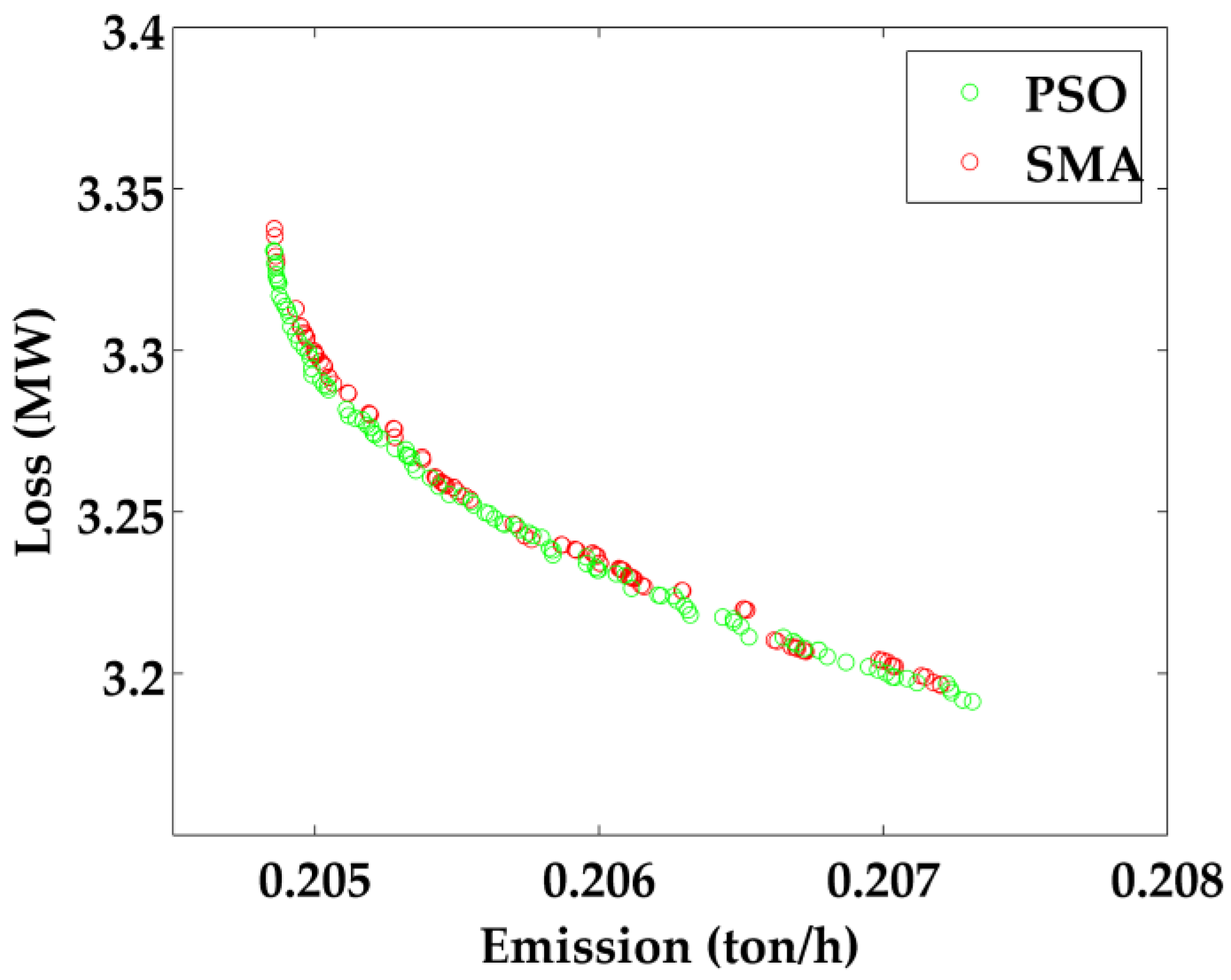
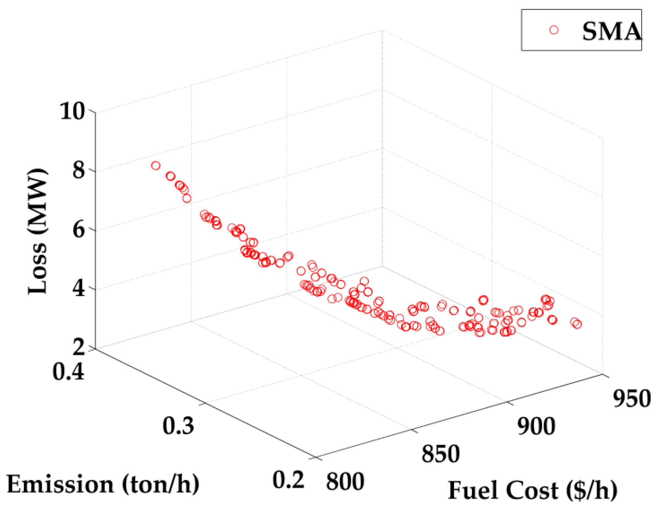
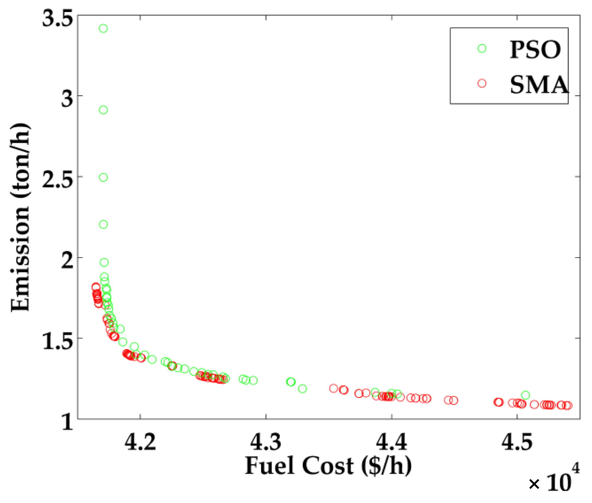
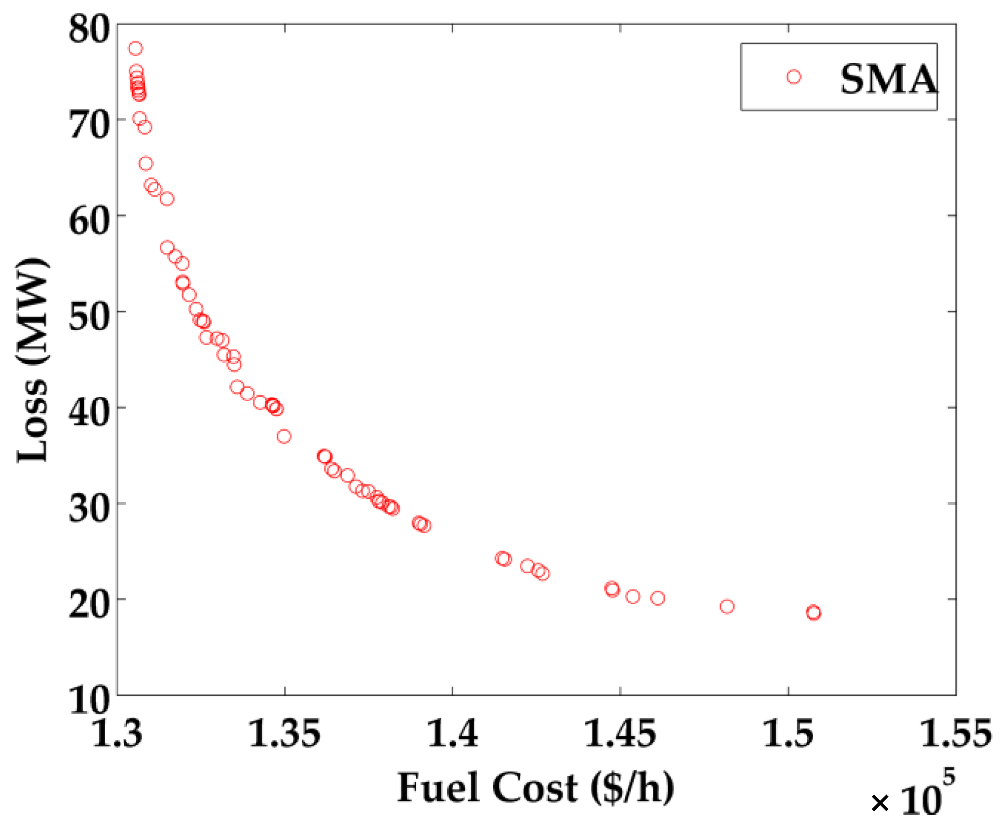
This paper presents a method to solve MOOPF problems based on SMA by considering fuel cost, emission, and transmission line loss as part of the objective functions to be minimized. The SMA is a recently proposed algorithm, which has been applied to successfully solve many optimization problems in several fields. However, the SMA has been rarely investigated on solving the single-objective OPF problem and never been evaluated on solving the MOOPF problem. So, this work has introduced a method to solve the MOOPF problems based on SMA and investigated the performance of the SMA on solving both single-objective and multi-objective OPF problems. The IEEE 30-, 57-, and 118-bus systems were employed to evaluate the performance of the SMA. The simulation results show that the SMA could successfully solve the single-objective OPF problem. The SMA provided slightly better solutions for the IEEE 30-bus system, moderately better solutions for the IEEE 57-bus system, and significantly better solutions for the IEEE 118-bus system in terms of the objective values than many other algorithms in the literature. For the MOOPF problems, the two-dimensional Pareto fronts generated by the SMA are better than those of the well-known high-performance algorithm which is the PSO algorithm. Especially in the IEEE 118-bus system, the SMA could efficiently obtain the Pareto fronts while PSO could not converge to the solutions within the imposed iteration. Moreover, the three-dimensional Pareto fronts could also be efficiently provided by the SMA where the operators should judiciously choose the appropriate solution depending on the objective and situation. Hence, the SMA is verified as a high-performance algorithm for solving both single-objective and multi-objective OPF problems, especially in large systems. In future work, the SMA can be applied to solve the OPF problems in practical systems where the system sizes are generally large, and many-objective OPF problems (more than three objective functions) can be solved based on SMA to further improve power system performance in several terms.

References

1. Biswas, P.P.; Suganthan, P.N.; Amaratunga, G.A.J. Optimal power flow solutions incorporating stochastic wind and solar power. Energy Convers. Manag. 2017, 148, 1194–1207. [Google Scholar] [CrossRef]
2. Mohagheghi, E.; Gabash, A.; Alramlawi, M.; Li, P. Real-time optimal power flow with reactive power dispatch of wind stations using a reconciliation algorithm. Renew. Energy 2018, 126, 509–523. [Google Scholar] [CrossRef]
3. Luo, J.; Shi, L.; Ni, Y. A solution of optimal power flow incorporating wind generation and power grid uncertainties. IEEE Access 2018, 6, 19681–19690. [Google Scholar] [CrossRef]
4. Ma, H.; Hart, J.L. Economic Dispatch in View of the Clean Air Act of 1990. IEEE Trans. Power Syst. 2000, 9, 972–978. [Google Scholar]
5. Roy, P.K.; Ghoshal, S.P.; Thakur, S.S. Biogeography based optimization for multi-constraint optimal power flow with emission and non-smooth cost function. Expert Syst. Appl. 2010, 37, 8221–8228. [Google Scholar] [CrossRef]
6. Burchett, R.C.; Happ, H.H.; Vierath, D.R. Quadratically Convergent Optimal Power Flow. IEEE Trans. Power Appar. Syst. 1984, PAS-103, 3267–3275. [Google Scholar] [CrossRef]
7. Yan, X.; Quintana, V.H. Improving an interior-point-based off by dynamic adjustments of step sizes and tolerances. IEEE Trans. Power Syst. 1999, 14, 709–716. [Google Scholar] [CrossRef]
8. Momoh, J.A.; El-Hawary, M.E.; Adapa, R. A review of selected optimal power flow literature to 1993 part I: Nonlinear and quadratic Programming Approaches. IEEE Trans. Power Syst. 1999, 14, 96–103. [Google Scholar] [CrossRef]
9. Yodphet, D.; Onlam, A.; Siritaratiwat, A.; Khunkitti, P. Electrical distribution system reconfiguration for power loss reduction by the Salp Swarm algorithm. Int. J. Smart Grid Clean Energy 2019, 8, 156–163. [Google Scholar] [CrossRef] [Green Version]
10. Chamchuen, S.; Siritaratiwat, A.; Fuangfoo, P.; Suthisopapan, P.; Khunkitti, P. High-Accuracy Power Quality Disturbance Classification Using the Adaptive ABC-PSO As Optimal Feature Selection Algorithm. Energies 2021, 14, 1238. [Google Scholar] [CrossRef]
11. Khaboot, N.; Srithapon, C.; Siritaratiwat, A.; Khunkitti, P. Increasing Benefits in High PV Penetration Distribution System by Using Battery Enegy Storage and Capacitor Placement Based on Salp Swarm Algorithm. Energies 2019, 12, 4817. [Google Scholar] [CrossRef] [Green Version]
12. Nuaekaew, K.; Artrit, P.; Pholdee, N.; Bureerat, S. Optimal reactive power dispatch problem using a two-archive multi-objective grey wolf optimizer. Expert Syst. Appl. 2017, 87, 79–89. [Google Scholar] [CrossRef]
13. Khunkitti, S.; Premrudeepreechacharn, S.; Siritaratiwat, A.; Watson, N.R. Power system voltage stability enhancement based on line voltage stability indices in heavily loaded and line outage contingency situations. Int. J. Eng. Res. Technol. 2020, 13, 1635–1648. [Google Scholar] [CrossRef]
14. Khunkitti, S.; Premrudeepreechacharn, S.; Chatthaworn, R.; Thasnas, N.; Khunkitti, P.; Siritaratiwat, A.; Watson, N.R. A comparison of the effectiveness of voltage stability indices in an optimal power flow. IEEJ Trans. Electr. Electron. Eng. 2019, 14, 534–544. [Google Scholar] [CrossRef]
15. Khunkitti, S.; Watson, N.; Chatthaworn, R.; Premrudeepreechacharn, S.; Siritaratiwat, A. An Improved DA-PSO Optimization Approach for Unit Commitment Problem. Energies 2019, 12, 2335. [Google Scholar] [CrossRef] [Green Version]
16. Boonluk, P.; Siritaratiwat, A.; Fuangfoo, P.; Khunkitti, S. Optimal siting and sizing of battery energy storage systems for distribution network of distribution system operators. Batteries 2020, 6, 56. [Google Scholar] [CrossRef]
17. Boonluk, P.; Khunkitti, S.; Fuangfoo, P.; Siritaratiwat, A. Optimal Siting and Sizing of Battery Energy Storage: Case Study Seventh Feeder at Nakhon Phanom Substation in Thailand. Energies 2021, 14, 1458. [Google Scholar] [CrossRef]
18. Diab, H.; Abdelsalam, M.; Abdelbary, A. A Multi-Objective Optimal Power Flow Control of Electrical Transmission Networks Using Intelligent Meta-Heuristic Optimization Techniques. Sustainability 2021, 13, 4979. [Google Scholar] [CrossRef]
19. Islam, M.Z.; Wahab, N.I.A.; Veerasamy, V.; Hizam, H.; Mailah, N.F.; Guerrero, J.M.; Mohd Nasir, M.N. A Harris Hawks optimization based singleand multi-objective optimal power flow considering environmental emission. Sustainability 2020, 12, 5248. [Google Scholar] [CrossRef]
20. Sliman, L.; Bouktir, T. Economic Power Dispatch of Power System with Pollution Control using Multiobjective Ant Colony Optimization. Int. J. Comput. Intell. Res. 2007, 3, 145–153. [Google Scholar] [CrossRef]
21. El-Fergany, A.A.; Hasanien, H.M. Single and Multi-objective Optimal Power Flow Using Grey Wolf Optimizer and Differential Evolution Algorithms. Electr. Power Compon. Syst. 2015, 43, 1548–1559. [Google Scholar] [CrossRef]
22. Shang, R.; Wang, Y.; Wang, J.; Jiao, L.; Wang, S.; Qi, L. A multi-population cooperative coevolutionary algorithm for multi-objective capacitated arc routing problem. Inf. Sci. 2014, 277, 609–642. [Google Scholar] [CrossRef]
23. Khunkitti, S.; Siritaratiwat, A.; Premrudeepreechacharn, S.; Chatthaworn, R.; Watson, N. A Hybrid DA-PSO Optimization Algorithm for Multiobjective Optimal Power Flow Problems. Energies 2018, 11, 2270. [Google Scholar] [CrossRef] [Green Version]
24. Ghasemi, M.; Ghavidel, S.; Ghanbarian, M.M.; Gitizadeh, M. Multi-objective optimal electric power planning in the power system using Gaussian bare-bones imperialist competitive algorithm. Inf. Sci. 2015, 294, 286–304. [Google Scholar] [CrossRef]
25. Shabanpour-Haghighi, A.; Seifi, A.; Niknam, T. A modified teaching-learning based optimization for multi-objective optimal power flow problem. Energy Convers. Manag. 2014, 77, 597–607. [Google Scholar] [CrossRef]
26. Niknam, T.; Narimani, M.R.; Jabbari, M.; Malekpour, A.R. A modified shuffle frog leaping algorithm for multi-objective optimal power flow. Energy 2011, 36, 6420–6432. [Google Scholar] [CrossRef]
27. Žilinskas, A.; Žilinskas, J. Adaptation of a one-step worst-case optimal univariate algorithm of bi-objective Lipschitz optimization to multidimensional problems. Commun. Nonlinear Sci. Numer. Simul. 2015, 21, 89–98. [Google Scholar] [CrossRef]
28. Žilinskas, A.; Fraga, E.S.; Mackute, A. Data analysis and visualisation for robust multi-criteria process optimisation. Comput. Chem. Eng. 2006, 30, 1061–1071. [Google Scholar] [CrossRef]
29. Nagar, D.; Ramu, P.; Deb, K. Interpretable Self-Organizing Maps (iSOM) for Visualization of Pareto Front in Multiple Objective Optimization. In Proceedings of the Evolutionary Multi-Criterion Optimization, 11th International Conference, EMO 2021, Shenzhen, China, 28–31 March 2021; pp. 645–655. [Google Scholar]
30. Mirjalili, S.; Mirjalili, S.M.; Lewis, A. Grey Wolf Optimizer. Adv. Eng. Softw. 2014, 69, 46–61. [Google Scholar] [CrossRef] [Green Version]
31. Mirjalili, S.; Lewis, A. The Whale Optimization Algorithm. Adv. Eng. Softw. 2016, 95, 51–67. [Google Scholar] [CrossRef]
32. Mirjalili, S.; Gandomi, A.H.; Mirjalili, S.Z.; Saremi, S.; Faris, H.; Mirjalili, S.M. Salp Swarm Algorithm: A bio-inspired optimizer for engineering design problems. Adv. Eng. Softw. 2017, 114, 163–191. [Google Scholar] [CrossRef]
33. Heidari, A.A.; Mirjalili, S.; Faris, H.; Aljarah, I.; Mafarja, M.; Chen, H. Harris hawks optimization: Algorithm and applications. Futur. Gener. Comput. Syst. 2019, 97, 849–872. [Google Scholar] [CrossRef]
34. Li, S.; Chen, H.; Wang, M.; Heidari, A.A.; Mirjalili, S. Slime mould algorithm: A new method for stochastic optimization. Futur. Gener. Comput. Syst. 2020, 111, 300–323. [Google Scholar] [CrossRef]
35. Kumar, C.; Raj, T.D.; Premkumar, M.; Raj, T.D. A new stochastic slime mould optimization algorithm for the estimation of solar photovoltaic cell parameters. Optik 2020, 223, 165277. [Google Scholar] [CrossRef]
36. Liu, M.; Li, Y.; Huo, Q.; Li, A.; Zhu, M.; Qu, N.; Chen, L.; Xia, M. A two-way parallel slime mold algorithm by flow and distance for the travelling salesman problem. Appl. Sci. 2020, 10, 6180. [Google Scholar] [CrossRef]
37. Zubaidi, S.L.; Abdulkareem, I.H.; Hashim, K.S.; Al-Bugharbee, H.; Ridha, H.M.; Gharghan, S.K.; Al-Qaim, F.F.; Muradov, M.; Kot, P.; Al-Khaddar, R. Hybridised artificial neural network model with slime mould algorithm: A novel methodology for prediction of urban stochastic water demand. Water 2020, 12, 2692. [Google Scholar] [CrossRef]
38. Kouadri, R.; Musirin, I.; Slimani, L.; Bouktir, T.; Othman, M.M. Optimal power flow control variables using slime mould algorithm for generator fuel cost and loss minimization with voltage profile enhancement solution. Int. J. Emerg. Trends Eng. Res. 2020, 8, 36–44. [Google Scholar] [CrossRef]
39. Niknam, T.; Narimani, M.R.; Aghaei, J.; Azizipanah-Abarghooee, R. Improved particle swarm optimisation for multi-objective optimal power flow considering the cost, loss, emission and voltage stability index. IET Gener. Transm. Distrib. 2012, 6, 515. [Google Scholar] [CrossRef]
40. Mirjalili, S.; Saremi, S.; Mirjalili, S.M.; Coelho, L.D.S. Multi-objective grey wolf optimizer: A novel algorithm for multi-criterion optimization. Expert Syst. Appl. 2016, 47, 106–119. [Google Scholar] [CrossRef]
41. The University of Washington Electrical Engineering. The University of Washington Electrical Engineering. Power System Test Case Archive, the IEEE 30-Bus Test System Data. Available online: https://www2.ee.washington.edu/research/pstca/pf30/pg_tca30bus.htm (accessed on 19 April 2021).
42. Yuryevich, J.; Wong, K.P. Evolutionary Programming Based Optimal Power Flow Algorithm. IEEE Trans. Power Syst. 1999, 14, 1245–1250. [Google Scholar] [CrossRef]
43. Bouktir, T.; Slimani, L.; Mahdad, B. Optimal Power Dispatch for Large Scale Power System Using Stochastic Search Algorithms. Int. J. Power Energy Syst. 2008, 28. [Google Scholar] [CrossRef]
44. Sood, Y. Evolutionary programming based optimal power flow and its validation for deregulated power system analysis. Int. J. Electr. Power Energy Syst. 2007, 29, 65–75. [Google Scholar] [CrossRef]
45. Abaci, K.; Yamacli, V. Differential search algorithm for solving multi-objective optimal power flow problem. Int. J. Electr. Power Energy Syst. 2016, 79, 1–10. [Google Scholar] [CrossRef]
46. Narimani, M.R.; Azizipanah-Abarghooee, R.; Zoghdar-Moghadam-Shahrekohne, B.; Gholami, K. A novel approach to multi-objective optimal power flow by a new hybrid optimization algorithm considering generator constraints and multi-fuel type. Energy 2013, 49, 119–136. [Google Scholar] [CrossRef]
47. Sivasubramani, S.; Swarup, K.S. Multi-objective harmony search algorithm for optimal power flow problem. Int. J. Electr. Power Energy Syst. 2011, 33, 745–752. [Google Scholar] [CrossRef]
48. The University of Washington Electrical Engineering. The University of Washington Electrical Engineering. Power System Test Case Archive, the IEEE 57-Bus Test System Data. Available online: https://www2.ee.washington.edu/research/pstca/pf57/pg_tca57bus.htm (accessed on 19 April 2021).
49. Vaisakh, K.; Srinivas, L.R. Evolving ant direction differential evolution for OPF with non-smooth cost functions. Eng. Appl. Artif. Intell. 2011, 24, 426–436. [Google Scholar] [CrossRef]
50. Hsiao, Y.T.; Chen, C.H.; Chien, C.C. Optimal capacitor placement in distribution systems using a combination fuzzy-GA method. Int. J. Electr. Power Energy Syst. 2004, 26, 501–508. [Google Scholar] [CrossRef]
51. Rezaei Adaryani, M.; Karami, A. Artificial bee colony algorithm for solving multi-objective optimal power flow problem. Int. J. Electr. Power Energy Syst. 2013, 53, 219–230. [Google Scholar] [CrossRef]
52. Mahdad, B.; Srairi, K. Hierarchical adaptive PSO for multi-objective OPF considering emissions based shunt FACTS. IECON Proc. (Ind. Electron. Conf.) 2012, 1337–1343. [Google Scholar] [CrossRef]
53. Selvakumar, A.I.; Thanushkodi, K. A new particle swarm optimization solution to nonconvex economic dispatch problems. IEEE Trans. POWER Syst. 2007, 22, 42–51. [Google Scholar] [CrossRef]
54. The Electrical and Computer Engineering Department, I.I. of T. The Electrical and Computer Engineering Department, Illinois Institute of Technology, Data, The IEEE 118-Bus Test System Data. Available online: http://motor.ece.iit.edu/data/JEAS_IEEE118.doc (accessed on 19 April 2021).
55. Bouchekara, H.R.E.H.; Abido, M.A.; Boucherma, M. Optimal power flow using Teaching-Learning-Based Optimization technique. Electr. Power Syst. Res. 2014, 114, 49–59. [Google Scholar] [CrossRef]
56. Pandiarajan, K.; Babulal, C.K. Fuzzy harmony search algorithm based optimal power flow for power system security enhancement. Int. J. Electr. Power Energy Syst. 2016, 78, 72–79. [Google Scholar] [CrossRef]
57. Bhattacharya, A.; Roy, P.K. Solution of multi-objective optimal power flow using gravitational search algorithm. IET Gener. Transm. Distrib. 2012, 6, 751. [Google Scholar] [CrossRef]
58. Radosavljević, J.; Klimenta, D.; Jevtić, M.; Arsić, N. Optimal Power Flow Using a Hybrid Optimization Algorithm of Particle Swarm Optimization and Gravitational Search Algorithm. Electr. Power Components Syst. 2015, 43, 1958–1970. [Google Scholar] [CrossRef]
59. Bouchekara, H.R.E.H.; Chaib, A.E.; Abido, M.A.; El-Sehiemy, R.A. Optimal power flow using an Improved Colliding Bodies Optimization algorithm. Appl. Soft Comput. J. 2016, 42, 119–131. [Google Scholar] [CrossRef]
60. Mohamed, A.-A.A.; Mohamed, Y.S.; El-Gaafary, A.A.M.; Hemeida, A.M. Optimal power flow using moth swarm algorithm. Electr. Power Syst. Res. 2017, 142, 190–206. [Google Scholar] [CrossRef]
61. Attia, A.F.; El Sehiemy, R.A.; Hasanien, H.M. Optimal power flow solution in power systems using a novel Sine-Cosine algorithm. Int. J. Electr. Power Energy Syst. 2018, 99, 331–343. [Google Scholar] [CrossRef]
Figure 1. Flow chart of slime mould algorithm (SMA) for solving multi-objective optimal power flow (MOOPF) problems.
Sustainability 13 07448 g001
Figure 2. Two-dimensional Pareto fronts for case 4.
Sustainability 13 07448 g002
Figure 3. Two-dimensional Pareto fronts for case 5.
Sustainability 13 07448 g003
Figure 4. Two-dimensional Pareto fronts for case 6.
Sustainability 13 07448 g004
Figure 5. Three-dimensional Pareto fronts for case 7.
Sustainability 13 07448 g005
Figure 6. Two-dimensional Pareto fronts for case 11.
Sustainability 13 07448 g006
Figure 7. Three-dimensional Pareto fronts for case 12.
Sustainability 13 07448 g007
Figure 8. Two-dimensional Pareto fronts for case 14.
Sustainability 13 07448 g008