Modeling of Low Visibility-Related Rural Single-Vehicle Crashes Considering Unobserved Heterogeneity and Spatial Correlation


Abstract
:1. Introduction
2. Background
2.1. Safety Covariates of Rural Single-Vehicle Crashes
2.2. Statistical Techniques for Unobserved Heterogeneity and Spatial Correlation
2.3. The Current Research
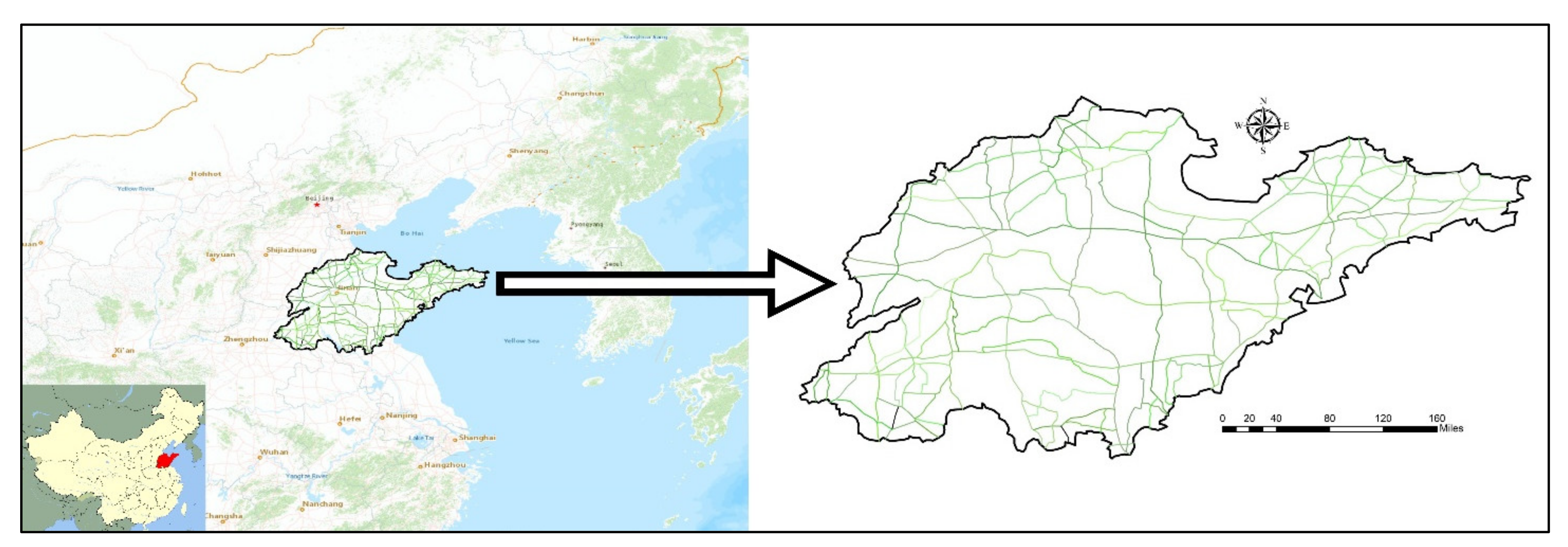
3. Data
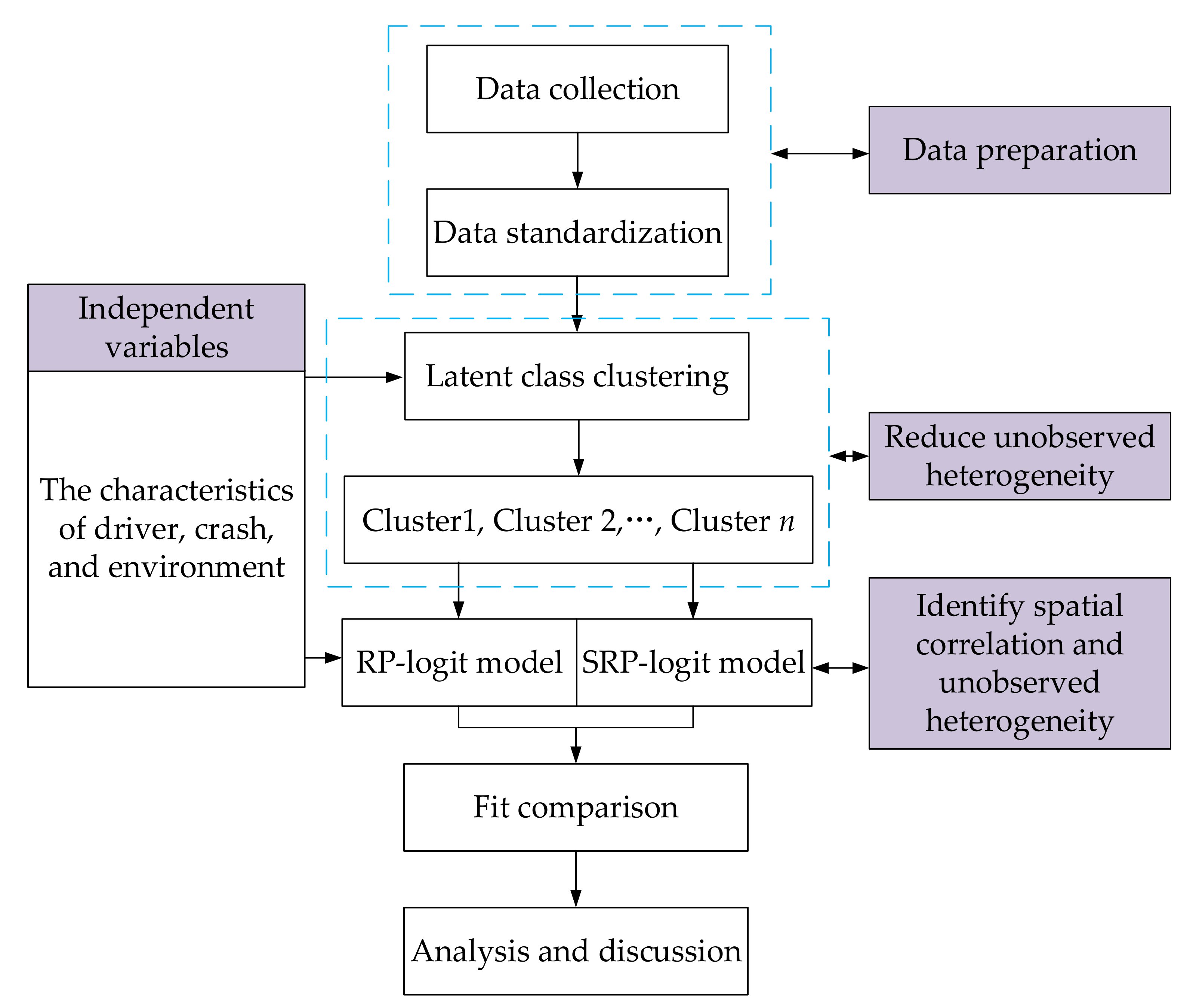
4. Methodology
4.1. Latent Class Clustering Model
4.2. Spatial Random Parameters Logit Model
4.3. Average Marginal Effect
5. Analysis and Discussion
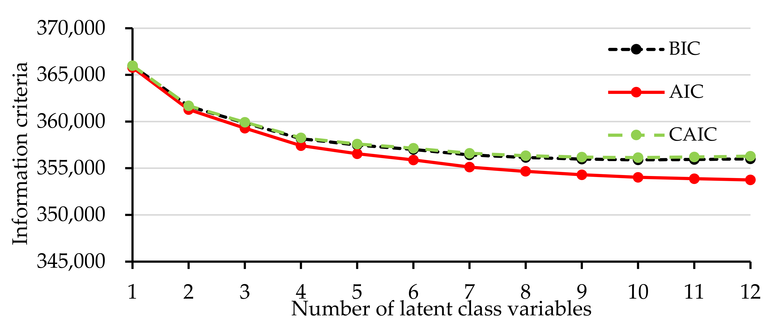
5.1. Analysis of Latent Class Clustering Model
5.2. Analysis of Spatial Random Parameters Logit Model
5.3. Discussion
5.3.1. Driver Characteristics
5.3.2. Vehicle Characteristics
5.3.3. Other Characteristics
5.4. Recommendations
6. Conclusions
7. Limitations of the Study
Author Contributions
Funding
Institutional Review Board Statement
Informed Consent Statement
Data Availability Statement
Acknowledgments
Conflicts of Interest
Appendix A

| Variables | Description | Cluster 1 | Cluster 2 | Cluster 3 | Cluster 4 |
|---|---|---|---|---|---|
| Number | 9517 | 3561 | 3075 | 2860 | |
| Injury severity | No injury | 9210 | 3377 | 46 | 675 |
| Slight injury | 253 | 105 | 1757 | 1655 | |
| FS injuries | 54 | 79 | 1272 | 530 | |
| Driver gender | Female | 12.3% | 0.1% | 2.6% | 21.7% |
| Male | 87.7% | 99.9% | 97.4% | 78.3% | |
| Driver age | <25 | 73.1% | 88.3% | 64.4% | 36.6% |
| [25,50] | 16.1% | 3.2% | 16.3% | 13.7% | |
| >50 | 10.8% | 8.5% | 19.3% | 49.7% | |
| Seatbelt/helmet | Used | 83.1% | 77.8% | 71.4% | 13.5% |
| Not used | 16.9% | 22.2% | 28.6% | 86.5% | |
| Drunk driving | No | 76.2% | 84.8% | 75.5% | 54.5% |
| Yes | 23.8% | 15.2% | 24.5% | 45.5% | |
| Career | Company staff | 16.6% | 16.2% | 14.8% | 16.5% |
| Self-employed | 38.4% | 26.3% | 25.5% | 19.5% | |
| Farmer | 36.9% | 49.4% | 50.9% | 49.4% | |
| Others | 8.2% | 8.1% | 8.9% | 14.7% | |
| Vehicle type | Passenger car | 81.2% | 12.7% | 17.5% | 1.2% |
| Motorcycle | 9.9% | 1.8% | 68.4% | 52.9% | |
| Pickup | 6.2% | 9.4% | 5.9% | 43.3% | |
| Truck | 0.1% | 68.2% | 7.4% | 0.1% | |
| Others | 2.7% | 7.9% | 0.8% | 2.7% | |
| Week | Monday/Friday | 43.4% | 45.2% | 44.2% | 43.7% |
| Tuesday–Thursday | 28.8% | 28.2% | 26.7% | 29.5% | |
| Weekend | 27.8% | 26.6% | 29.1% | 26.9% | |
| Intersection | No | 64.9% | 64.8% | 76.1% | 57.4% |
| Yes | 35.0% | 35.1% | 23.9% | 42.6% | |
| Time of day | 00:00–7:00 | 15.0% | 16.1% | 6.2% | 16.4% |
| 7:00–10:00 | 35.1% | 33.6% | 26.3% | 36.9% | |
| 10:00–17:00 | 23.7% | 15.9% | 17.6% | 20.2% | |
| 17:00–21:00 | 17.1% | 11.0% | 30.3% | 14.7% | |
| 21:00–24:00 | 9.2% | 23.3% | 19.7% | 11.8% | |
| Collision type | Collision with fixed object | 75.3% | 82.6% | 55.9% | 83.5% |
| Collision with non-fixed object | 2.5% | 3.6% | 40.2% | 3.3% | |
| Collision with pedestrian | 22.2% | 13.5% | 3.8% | 13.2% | |
| Others | 0.1% | 0.3% | 0.9% | 0.8% | |
| Traffic control | No control | 50.0% | 59.5% | 54.5% | 59.5% |
| Control | 49.9% | 40.5% | 45.5% | 40.5% |
References
- National Highway Traffic Safety Administration (NHTSA). Traffic Safety Facts Annual Report Tables. 2018. Available online: https://cdan.nhtsa.gov/tsftables/tsfar.htm# (accessed on 15 June 2021).
- Yan, X.; He, J.; Zhang, C.; Liu, Z.; Qiao, B.; Zhang, H. Single-vehicle crash severity outcome prediction and determinant extraction using tree-based and other non-parametric models. Accid. Anal. Prev. 2021, 153, 106034. [Google Scholar] [CrossRef]
- Traffic Management Bureau of Ministry of Public Security of China. Statistics Annals of Road Traffic Accident of People’s Republic of China (2017); Traffic Management Science Institute of Ministry of Public Security: Wuxi, China, 2018.
- Chen, Y.; Luo, R.; Yang, H.; King, M.; Shi, Q. Applying latent class analysis to investigate rural highway single-vehicle fatal crashes in China. Accid. Anal. Prev. 2020, 148, 105840. [Google Scholar] [CrossRef]
- Li, Z.; Ci, Y.; Chen, C.; Zhang, G.; Wu, Q.; Qian, Z.; Prevedouros, P.D.; Ma, D.T. Investigation of driver injury severities in rural single-vehicle crashes under rain conditions using mixed logit and latent class models. Accid. Anal. Prev. 2019, 124, 219–229. [Google Scholar] [CrossRef]
- Yu, H.; Yuan, R.; Li, Z.; Zhang, G.; Ma, D.T. Identifying heterogeneous factors for driver injury severity variations in snow-related rural single-vehicle crashes. Accid. Anal. Prev. 2020, 144, 105587. [Google Scholar] [CrossRef]
- Xu, C.; Tarko, A.P.; Wang, W.; Liu, P. Predicting crash likelihood and severity on freeways with real-time loop detector data. Accid. Anal. Prev. 2013, 57, 30–39. [Google Scholar] [CrossRef] [PubMed]
- Wu, Q.; Chen, F.; Zhang, G.; Liu, X.C.; Wang, H.; Bogus, S.M. Mixed logit model-based driver injury severity investigations in single-and multi-vehicle crashes on rural two-lane highways. Accid. Anal. Prev. 2014, 72, 105–115. [Google Scholar] [CrossRef] [PubMed]
- Wu, Q.; Zhang, G.; Zhu, X.; Liu, X.C.; Tarefder, R. Analysis of driver injury severity in single-vehicle crashes on rural and urban roadways. Accid. Anal. Prev. 2016, 94, 35–45. [Google Scholar] [CrossRef] [PubMed]
- Yu, H.; Li, Z.; Zhang, G.; Liu, P. A latent class approach for driver injury severity analysis in highway single vehicle crash considering unobserved heterogeneity and temporal influence. Anal. Methods Accid. Res. 2019, 24, 100110. [Google Scholar] [CrossRef]
- Xu, C.; Wang, W.; Liu, P. A genetic programming model for real-time crash prediction on freeways. IEEE T Intell. Transp. 2012, 14, 574–586. [Google Scholar] [CrossRef]
- Shangguan, Q.; Fu, T.; Liu, S. Investigating rear-end collision avoidance behavior under varied foggy weather conditions: A study using advanced driving simulator and survival analysis. Accid. Anal. Prev. 2020, 139, 105499. [Google Scholar] [CrossRef]
- Ma, D.; Xiao, J.; Ma, X. A decentralized model predictive traffic signal control method with fixed phase sequence for urban networks. J. Intell. Transport. S. 2020. [Google Scholar] [CrossRef]
- Wen, H.; Xue, G. Injury severity analysis of familiar drivers and unfamiliar drivers in single-vehicle crashes on the mountainous highways. Accid. Anal. Prev. 2020, 144, 105667. [Google Scholar] [CrossRef] [PubMed]
- Wei, F.; Cai, Z.; Guo, Y.; Liu, P.; Wang, Z.; Li, Z. Analysis of roadside accident severity on rural and urban roadways. Intell. Autom. Soft Comput. 2021, 28, 753–767. [Google Scholar] [CrossRef]
- Li, Z.; Chen, C.; Wu, Q.; Zhang, G.; Liu, C.; Prevedouros, P.D.; Ma, D.T. Exploring driver injury severity patterns and causes in low visibility related single-vehicle crashes using a finite mixture random parameters model. Anal. Methods Accid. Res. 2018, 20, 1–14. [Google Scholar] [CrossRef]
- Ma, D.; Song, X.; Li, P. Daily traffic flow forecasting through a contextual convolutional recurrent neural network modeling inter-and intra-day traffic patterns. IEEE T Intell. Transp. 2021, 22, 2627–2636. [Google Scholar] [CrossRef]
- Guo, Y.; Sayed, T.; Essa, M. Real-time conflict-based Bayesian Tobit models for safety evaluation of signalized intersections. Accid. Anal. Prev. 2020, 144, 105660. [Google Scholar] [CrossRef]
- Qin, L.; Li, Z.R.; Chen, Z.; Bill, A.; Noyce, D.A. Understanding driver distractions in fatal crashes: An exploratory empirical analysis. J. Saf. Res. 2019, 69, 23–31. [Google Scholar] [CrossRef] [PubMed]
- Choudhary, P.; Pawar, N.M.; Velaga, N.R.; Pawar, D.S. Overall performance impairment and crash risk due to distracted driving: A comprehensive analysis using structural equation modelling. Transp. Res. Part F Traffic Psychol. Behav. 2020, 74, 120–138. [Google Scholar] [CrossRef]
- Xie, Y.; Zhao, K.; Huynh, N. Analysis of driver injury severity in rural single–vehicle crashes. Accid. Anal. Prev. 2012, 47, 36–44. [Google Scholar] [CrossRef]
- Adanu, E.K.; Hainen, A.; Jones, S. Latent class analysis of factors that influence weekday and weekend single-vehicle crash severities. Accid. Anal. Prev. 2018, 113, 187–192. [Google Scholar] [CrossRef]
- Rahimi, E.; Shamshiripour, A.; Samimi, A.; Mohammadian, A. Investigating the injury severity of single-vehicle truck crashes in a developing country. Accid. Anal. Prev. 2020, 137, 105444. [Google Scholar] [CrossRef]
- Haq, M.T.; Zlatkovic, M.; Ksaibati, K. Investigating occupant injury severity of truck-involved crashes based on vehicle types on a mountainous freeway: A hierarchical Bayesian random intercept approach. Accid. Anal. Prev. 2020, 144, 105654. [Google Scholar] [CrossRef]
- Anarkooli, A.J.; Hosseinpour, M.; Kardar, A. Investigation of factors affecting the injury severity of single-vehicle rollover crashes: A random-effects generalized ordered probit model. Accid. Anal. Prev. 2017, 106, 399–410. [Google Scholar] [CrossRef]
- Rezapour, M.; Moomen, M.; Ksaibati, K. Ordered logistic models of influencing factors on crash injury severity of single and multiple-vehicle downgrade crashes: A case study in Wyoming. J. Saf. Res. 2019, 68, 107–118. [Google Scholar] [CrossRef] [PubMed]
- Vajari, M.A.; Aghabayk, K.; Sadeghian, M.; Shiwakoti, N. A multinomial logit model of motorcycle crash severity at Australian intersections. J. Saf. Res. 2020, 73, 17–24. [Google Scholar] [CrossRef] [PubMed]
- Islam, S.; Jones, S.L.; Dye, D. Comprehensive analysis of single- and multi-vehicle large truck at-fault crashes on rural and urban roadways in Alabama. Accid. Anal. Prev. 2014, 67, 148–158. [Google Scholar] [CrossRef]
- Lee, J.; Yasmin, S.; Eluru, N.; Abdel-Aty, M.; Cai, Q. Analysis of crash proportion by vehicle type at traffic analysis zone level: A mixed fractional split multinomial logit modeling approach with spatial effects. Accid. Anal. Prev. 2018, 111, 12–22. [Google Scholar] [CrossRef] [PubMed]
- Rusli, R.; Haque, M.M.; King, M.; Voon, W.S. Single-vehicle crashes along rural mountainous highways in Malaysia: An application of random parameters negative binomial model. Accid. Anal. Prev. 2017, 102, 153–164. [Google Scholar] [CrossRef] [Green Version]
- Hou, Q.; Huo, X.; Leng, J.; Cheng, Y. Examination of driver injury severity in freeway single-vehicle crashes using a mixed logit model with heterogeneity-in-means. Physica A 2017, 531, 121760. [Google Scholar] [CrossRef]
- Duddu, V.R.; Pulugurtha, S.S.; Kukkapalli, V.M. Variable categories influencing single-vehicle run-off-road crashes and their severity. Transp. Eng. 2020, 2, 100038. [Google Scholar] [CrossRef]
- Yu, H.; Li, Z.; Zhang, G.; Liu, P.; Ma, T. Fusion convolutional neural network-based interpretation of unobserved heterogeneous factors in driver injury severity outcomes in single-vehicle crashes. Anal. Methods Accid. Res. 2021, 30, 100157. [Google Scholar] [CrossRef]
- Mannering, F.L.; Shankar, V.; Bhat, C.R. Unobserved heterogeneity and the statistical analysis of highway accident data. Anal. Methods Accid. Res. 2016, 11, 1–16. [Google Scholar] [CrossRef]
- Li, Z.; Wang, W.; Liu, P.; Bigham, J.M.; Ragland, D.R. Using geographically weighted Poisson regression for county-level crash modeling in California. Saf. Sci. 2013, 58, 89–98. [Google Scholar] [CrossRef]
- Xu, C.; Liu, P.; Wang, W.; Zhang, Y. Real-time identification of traffic conditions prone to injury and non-injury crashes on freeways using genetic programming. J. Adv. Transport. 2016, 50, 701–716. [Google Scholar] [CrossRef] [Green Version]
- Xu, C.; Liu, P.; Wang, W.; Li, Z. Evaluation of the impacts of traffic states on crash risks on freeways. Accid. Anal. Prev. 2012, 47, 162–171. [Google Scholar] [CrossRef] [PubMed]
- Roque, C.; Jalayer, M.; Hasan, A.S. Investigation of injury severities in single-vehicle crashes in North Carolina using mixed logit models. J. Saf. Res. 2021, 77, 161–169. [Google Scholar] [CrossRef]
- Guo, Y.; Wu, Y.; Lu, J.; Zhou, J. Modeling the unobserved heterogeneity in e-bike collision severity using full bayesian random parameters multinomial logit regression. Sustainability 2019, 11, 2071. [Google Scholar] [CrossRef] [Green Version]
- Tay, R. A random parameters probit model of urban and rural intersection crashes. Accid. Anal. Prev. 2015, 84, 38–40. [Google Scholar] [CrossRef]
- Xu, C.; Wang, W.; Liu, P. Identifying crash-prone traffic conditions under different weather on freeways. J. Saf. Res. 2013, 46, 135–144. [Google Scholar] [CrossRef]
- Buddhavarapu, P.; Scott, J.G.; Prozzi, J.A. Modeling unobserved heterogeneity using finite mixture random parameters for spatially correlated discrete count data. Transport. Res. Part B Methodol. 2016, 91, 492–510. [Google Scholar] [CrossRef]
- Mannering, F.L.; Bhat, C.R. Analytic methods in accident research: Methodological frontier and future directions. Anal. Methods Accid. Res. 2014, 1, 1–22. [Google Scholar] [CrossRef]
- Guo, Y.; Liu, P.; Wu, Y.; Chen, J. Evaluating how right-turn treatments affect right-turn-on-red conflicts at signalized intersections. J. Transp. Saf. Secur. 2020, 12, 419–440. [Google Scholar] [CrossRef]
- Guo, Y.; Sayed, T.; Zheng, L. A hierarchical Bayesian peak over threshold approach for conflict-based before-after safety evaluation of leading pedestrian intervals. Accid. Anal. Prev. 2020, 147, 105772. [Google Scholar] [CrossRef]
- Azimi, G.; Rahimi, A.; Asgari, H.; Jin, X. Severity analysis for large truck rollover crashes using a random parameter ordered logit model. Accid. Anal. Prev. 2020, 135, 105355. [Google Scholar] [CrossRef] [PubMed]
- Yu, M.; Zheng, C.; Ma, C.; Shen, J. The temporal stability of factors affecting driver injury severity in run-off-road crashes: A random parameters ordered probit model with heterogeneity in the means approach. Accid. Anal. Prev. 2020, 144, 105677. [Google Scholar] [CrossRef] [PubMed]
- Cerwick, D.M.; Gkritza, K.; Shaheed, M.S.; Hans, Z. A comparison of the mixed logit and latent class methods for crash severity analysis. Anal. Methods Accid. Res. 2014, 3–4, 11–27. [Google Scholar] [CrossRef]
- Chen, C.; Zhang, G.; Tian, Z.; Bogus, S.M.; Yang, Y. Hierarchical Bayesian random intercept model-based cross-level interaction decomposition for truck driver injury severity investigations. Accid. Anal. Prev. 2015, 85, 186–198. [Google Scholar] [CrossRef] [PubMed]
- Guo, Y.; Li, Z.; Liu, P.; Wu, Y. Modeling correlation and heterogeneity in crash rates by collision types using full bayesian random parameters multivariate Tobit model. Accid. Anal. Prev. 2019, 128, 164–174. [Google Scholar] [CrossRef]
- Ma, D.; Xiao, J.; Song, X.; Ma, X.; Jin, S. A back-pressure-based model with fixed phase sequences for traffic signal optimization under oversaturated networks. IEEE Trans. Intell. Transp. 2020, 99, 1–12. [Google Scholar] [CrossRef]
- Chang, F.; Xu, P.; Zhou, H.; Chan, A.H.S.; Huang, H. Investigating injury severities of motorcycle riders: A two-step method integrating latent class cluster analysis and random parameters logit model. Accid. Anal. Prev. 2019, 131, 316–326. [Google Scholar] [CrossRef]
- Li, Z.; Chen, C.; Ci, Y.; Zhang, G.; Wu, Q.; Liu, C.; Qian, Z. Examining driver injury severity in intersection-related crashes using cluster analysis and hierarchical Bayesian models. Accid. Anal. Prev. 2018, 120, 139–151. [Google Scholar] [CrossRef] [PubMed]
- Li, Z.; Wu, Q.; Ci, Y.; Chen, C.; Chen, X.; Zhang, G. Using latent class analysis and mixed logit model to explore risk factors on driver injury severity in single-vehicle crashes. Accid. Anal. Prev. 2019, 129, 230–240. [Google Scholar] [CrossRef] [PubMed]
- Liu, P.; Fan, W.D. Exploring injury severity in head-on crashes using latent class clustering analysis and mixed logit model: A case study of North Carolina. Accid. Anal. Prev. 2020, 135, 105388. [Google Scholar] [CrossRef]
- Zeng, Q.; Wen, H.; Huang, H.; Wang, J.; Lee, J. Analysis of crash frequency using a Bayesian underreporting count model with spatial correlation. Physica A 2020, 545, 123754. [Google Scholar] [CrossRef]
- Guo, Y.; Sayed, T.; Zheng, L.; Essa, M. An extreme value theory based approach for calibration of microsimulation models for safety analysis. Simul. Model. Pract. Theory 2021, 106, 102172. [Google Scholar] [CrossRef]
- Bi, H.; Ye, Z. Exploring ride sourcing trip patterns by fusing multi-source data: A big data approach. Sustain. Cities Soc. 2021, 64, 102499. [Google Scholar] [CrossRef]
- Yang, D.; Xie, K.; Ozbay, K.; Yang, H. Fusing crash data and surrogate safety measures for safety assessment: Development of a structural equation model with conditional autoregressive spatial effect and random parameters. Accid. Anal. Prev. 2021, 152, 105971. [Google Scholar] [CrossRef] [PubMed]
- Zeng, Q.; Gu, W.; Zhang, X.; Wen, H.; Lee, J.; Hao, W. Analyzing freeway crash severity using a Bayesian spatial generalized ordered logit model with conditional autoregressive priors. Accid. Anal. Prev. 2019, 127, 87–95. [Google Scholar] [CrossRef]
- Klassen, J.; El-Basyouny, K.; Islam, M.T. Analyzing the severity of bicycle-motor vehicle collision using spatial mixed logit models: A city of Edmonton case study. Saf. Sci. 2014, 62, 295–304. [Google Scholar] [CrossRef]
- Munira, S.; Sener, I.N.; Dai, B. A Bayesian spatial Poisson-lognormal model to examine pedestrian crash severity at signalized intersections. Accid. Anal. Prev. 2020, 144, 105679. [Google Scholar] [CrossRef]
- Cai, Q.; Abdel-Aty, M.; Lee, J.; Wang, L.; Wang, X. Developing a grouped random parameters multivariate spatial model to explore zonal effects for segment and intersection crash modeling. Anal. Methods Accid. Res. 2018, 19, 1–15. [Google Scholar] [CrossRef]
- Zeng, Q.; Wen, H.; Huang, H.; Abdel-Aty, M. A Bayesian spatial random parameters Tobit model for analyzing crash rates on roadway segments. Accid. Anal. Prev. 2017, 100, 37–43. [Google Scholar] [CrossRef]
- Huang, H.; Chang, F.; Zhou, H.; Lee, J. Modeling unobserved heterogeneity for zonal crash frequencies: A Bayesian multivariate random-parameters model with mixture components for spatially correlated data. Anal. Methods Accid. Res. 2019, 24, 100105. [Google Scholar] [CrossRef]
- Linzer, D.A.; Lewis, J. poLCA: An R Package for polytomous variable latent class analysis. J. Stat. Softw. 2011, 42, 1–29. [Google Scholar] [CrossRef] [Green Version]
- Xu, X.; Xie, S.; Wong, S.C.; Xu, P.; Huang, H.; Pei, X. Severity of pedestrian injuries due to traffic crashes at signalized intersections in Hong Kong: A Bayesian spatial logit model. J. Adv. Transport. 2017, 50, 2015–2028. [Google Scholar] [CrossRef]
- Banerjee, S.; Carlin, B.P.; Gelfand, A.E. Hierarchical Modeling and Analysis for Spatial Data, 2rd ed.; Chapman & Hall; CRC Press: Boca Raton, FL, USA, 2014. [Google Scholar]
- Dong, N.; Huang, H.; Xu, P.; Ding, Z.; Wang, D. Evaluating spatial-proximity structures in crash prediction models at the level of traffic analysis zones. Transp. Res. Rec. 2014, 2432, 46–52. [Google Scholar] [CrossRef]
- Aguero-Valverde, J.; Jovanis, P. Spatial correlation in multilevel crash frequency models: Effects of different neighboring structures. Transport. Res. Rec. 2010, 2165, 21–32. [Google Scholar] [CrossRef]
- El-Basyouny, K.; Sayed, T. Urban arterial accident prediction models with spatial effects. Transport. Res. Rec. 2009, 2102, 27–33. [Google Scholar] [CrossRef]
- Guo, Y.; Osama, A.; Sayed, T. A cross-comparison of different techniques for modeling macro-level cyclist crashes. Accid. Anal. Prev. 2018, 113, 38–46. [Google Scholar] [CrossRef]
- Feng, S.; Li, Z.; Ci, Y.; Zhang, G. Risk factors affecting fatal bus accident severity: Their impact on different types of bus drivers. Accid. Anal. Prev. 2016, 86, 29–39. [Google Scholar] [CrossRef]
- Naik, B.; Tung, L.W.; Zhao, S.; Khattak, A.J. Weather impacts on single-vehicle truck crash injury severity. J. Saf. Res. 2016, 58, 57–65. [Google Scholar] [CrossRef] [PubMed]
- Abdel-Aty, M.; Ekram, A.; Huang, H.; Choi, K. A study on crashes related to visibility obstruction due to fog and smoke. Accid. Anal. Prev. 2011, 43, 1730–1737. [Google Scholar] [CrossRef] [PubMed]
- Bédard, M.; Guyatt, G.H.; Stones, M.J.; Hirdes, J.P. The independent contribution of driver, crash, and vehicle characteristics to driver fatalities. Accid. Anal. Prev. 2002, 34, 717–727. [Google Scholar] [CrossRef]
- Zhang, T.; Chan, A.H.; Zhang, W. Dimensions of driving anger and their relationships with aberrant driving. Accid. Anal. Prev. 2015, 81, 124–133. [Google Scholar] [CrossRef] [PubMed]
- Zhu, X.; Srinivasan, S. A comprehensive analysis of factors influencing the injury severity of large-truck crashes. Accid. Anal. Prev. 2011, 43, 49–57. [Google Scholar] [CrossRef] [PubMed]

| Variables | Description | Number | Driver Injury Severity | ||
|---|---|---|---|---|---|
| No Injury | Slight Injury | FS Injuries | |||
| Total number | 19,014 | 70.0% | 20.1% | 9.8% | |
| Driver gender | Male | 17,209 | 70.6% | 19.3% | 10.1% |
| Female * | 1804 | 64.7% | 26.7% | 8.5% | |
| Driver age | <25 | 2473 | 67.6% | 23.8% | 8.4% |
| [25,50] * | 13,210 | 76.1% | 16.0% | 7.9% | |
| >50 | 3330 | 47.9% | 32.8% | 19.2% | |
| Seatbelt/helmet | Not used | 5778 | 50.9% | 32.4% | 16.5% |
| Used * | 13,235 | 78.4% | 14.5% | 6.9% | |
| Drunk driving | No * | 14,200 | 72.9% | 17.9% | 9.2% |
| Yes | 4813 | 58.7% | 26.1% | 15.1% | |
| Career | Company staff * | 3080 | 70.0% | 20.5% | 9.5% |
| Self-employed | 5869 | 77.0% | 15.7% | 7.2% | |
| Farmer | 8305 | 66.6% | 22.1% | 11.3% | |
| Others | 1759 | 63.0% | 23.3% | 13.6% | |
| Vehicle type | Passenger car * | 8405 | 90.3% | 6.9% | 2.7% |
| Motorcycle | 4574 | 29.0% | 47.0% | 23.8% | |
| Pickup | 2356 | 50.3% | 34.7% | 14.8% | |
| Truck | 3011 | 87.6% | 6.5% | 5.8% | |
| Others | 667 | 86.9% | 7.7% | 5.2% | |
| Week | Monday/Friday | 5405 | 70.7% | 19.7% | 9.6% |
| Tuesday–Thursday * | 8361 | 70.0% | 20.2% | 9.8% | |
| Weekend | 5247 | 69.3% | 19.9% | 10.8% | |
| Intersection | No * | 12,476 | 69.5% | 19.9% | 10.6% |
| Yes | 6537 | 71.0% | 20.2% | 8.8% | |
| Time of day | 00:00–7:00 | 2720 | 64.8% | 19.7% | 15.4% |
| 7:00–10:00 * | 2666 | 77.3% | 16.2% | 6.4% | |
| 10:00–17:00 | 6391 | 72.2% | 19.4% | 8.2% | |
| 17:00–21:00 | 3898 | 73.6% | 19.4% | 6.9% | |
| 21:00–24:00 | 3338 | 60.3% | 25.0% | 14.6% | |
| Collision type | Fixed object | 14,249 | 72.2% | 21.0% | 6.6% |
| Non-fixed object * | 1704 | 22.1% | 30.8% | 46.9% | |
| Pedestrian | 3042 | 89.4% | 8.3% | 2.2% | |
| Others | 18 | 50.1% | 44.7% | 5.2% | |
| Traffic control | No control * | 10,306 | 69.2% | 20.6% | 10.2% |
| Control | 8707 | 71.0% | 19.3% | 9.6% | |
| Variables | Cluster 1 | Cluster 2 | Cluster 3 | Cluster 4 |
|---|---|---|---|---|
| Number of observations | 9517 | 3561 | 3075 | 2860 |
| Older driver (>50) | 10.8% | 8.5% | 19.3% | 49.7% |
| Seatbelt/helmet used | 83.1% | 77.8% | 71.4% | 13.5% |
| Seatbelt/helmet not used | 16.9% | 22.3% | 28.6% | 86.5% |
| Drunk driving | 23.7% | 15.2% | 24.5% | 45.5% |
| Passenger car | 81.2% | 12.7% | 17.5% | 1.2% |
| Motorcycle | 9.8% | 1.8% | 68.4% | 52.9% |
| Truck | 0.2% | 68.2% | 7.4% | 0.03% |
| Collision with fixed object | 2.5% | 3.6% | 40.2% | 3.3% |
| Mid-age driver (25–50) | 73.1% | 88.3% | 64.3% | 33.6% |
| Categories | Total Sample Size | No Injury | Slight Injury | FS Injuries |
|---|---|---|---|---|
| Whole-dataset | 19,013 | 13,309 (70.0%) | 3802 (20.1%) | 1902 (9.8%) |
| Cluster 1 | 9517 | 9264 (97.3%) | 253 (2.6%) | 0 (0%) |
| Cluster 2 | 3561 | 3377 (94.8%) | 105 (2.9%) | 79 (2.2%) |
| Cluster 3 | 3075 | 46 (1.5%) | 1757 (57.1%) | 1272 (41.4%) |
| Cluster 4 | 2860 | 675 (23.6%) | 1655 (57.8%) | 530 (18.5%) |
| Indicators | Distribution Form | Whole-Dataset | Cluster 1 | Cluster 2 | Cluster 3 | Cluster 4 |
|---|---|---|---|---|---|---|
| Number | - | 19,013 | 9517 | 3561 | 3075 | 2860 |
| LL(β) | Normal distribution | −13,762.75 | −5661.29 | −3285.78 | −2632.22 | −2168.51 |
| Uniform distribution | −13,768.13 | −5674.34 | −3283.78 | −2641.53 | −2179.42 | |
| BIC | Normal distribution | 20,490.35 | 9084.12 | 4291.55 | 3971.34 | 3067.85 |
| Uniform distribution | 20,506.58 | 9095.87 | 4291.55 | 3988.25 | 3071.32 | |
| McFadden R2 | Normal distribution | 0.342 | 0.401 | 0.397 | 0.371 | 0.408 |
| Uniform distribution | 0.339 | 0.400 | 0.397 | 0.364 | 0.406 | |
| p-value | Normal distribution | <0.001 | ||||
| Uniform distribution | <0.001 | |||||
| Crash Dataset | BIC | ||
|---|---|---|---|
| RP-Logit Model | SRP-Logit Model | Difference | |
| Whole-dataset | 20,563.21 | 20,490.35 | 72.86 |
| Cluster 1 | 9109.08 | 9084.12 | 24.96 |
| Cluster 2 | 4309.86 | 4291.55 | 18.31 |
| Cluster 3 | 3983.92 | 3971.34 | 12.58 |
| Cluster 4 | 3072.02 | 3067.85 | 16.17 |
| Severity | Whole-Dataset | Cluster 1 | Cluster 2 | Cluster 3 | Cluster 4 |
|---|---|---|---|---|---|
| No injury | 1.067 * | 0.731 * | 2.549 ** | ||
| Slight injury | 0.814 ** | 0.415 *** | 0.612 * | 1.013 * | |
| FS injuries | 1.261 * | 2.164 ** | 0.321 *** |
| Variables | Whole-Dataset | Cluster 1 | Cluster 2 | Cluster 3 | Cluster 4 | ||||
|---|---|---|---|---|---|---|---|---|---|
| S | F | S | S | F | S | F | S | F | |
| Male driver | −0.63 ** | −0.28 *** | −0.29 * | −1.51 *** | 0.31 * | 1.40 ** | |||
| Std. dev. | 0.50 | 0.42 | |||||||
| Young (<25) | −0.39 ** | −0.59 ** | −0.60 * | −0.56 ** | 0.82 ** | ||||
| Std. dev. | 1.06 | ||||||||
| Old (>50) | 0.62 ** | 1.06 *** | 0.81 ** | −1.58 * | −1.34 ** | 1.58 * | 0.88 *** | ||
| Seatbelt not used | 0.71 * | 1.24 ** | 0.99 ** | 0.68 ** | 1.05 ** | 1.79 ** | −1.17 ** | ||
| Drunk driving | 0.33 ** | 0.31 ** | 0.35 * | −2.64 *** | 1.04 * | 2.68 * | −0.22 * | 0.35 ** | |
| Std. dev. | 1.25 | 1.21 | |||||||
| Self-employed | −0.41 ** | −0.52 ** | −0.13 * | ||||||
| Farmer | −0.17 * | −0.32 * | −0.43 * | ||||||
| Motorcycle | 3.07 ** | 3.32 *** | 0.41 * | 0.70 * | 3.42 ** | 2.45 * | |||
| Pickup | −1.97 ** | −1.12 ** | −2.21 ** | −0.59 * | −1.22 ** | 2.407 * | |||
| Std. dev. | 2.24 | 0.52 | |||||||
| Truck | −0.73 ** | −0.43 * | −0.46 * | −1.30 * | |||||
| Others | 0.49 * | ||||||||
| 10:00–17:00 | 0.22 * | ||||||||
| Std. dev. | 0.53 | ||||||||
| 17:00–21:00 | 0.27 * | 0.38 * | |||||||
| Std. dev. | 1.28 | 2.45 | |||||||
| 21:00–24:00 | 0.93 ** | 1.28 ** | −0.89 ** | 1.29 *** | 0.34 ** | 0.35 * | 0.60 ** | ||
| 0:00–7:00 | 0.68 ** | 1.26 *** | −1.29 ** | 1.08 ** | 2.63 *** | 0.26 ** | |||
| Control | 0.20 * | 0.38 ** | |||||||
| Fixed object | 1.89 ** | 3.64 ** | 1.71 ** | 1.64 *** | 1.70 * | 2.52 * | |||
| Std. dev. | 1.51 | ||||||||
| Pedestrian | −1.77 ** | −2.08 * | −0.56 ** | −1.41 ** | −0.60 ** | ||||
| Others | 3.29 ** | 3.34 ** | |||||||
| Intercept | −2.56 *** | −4.91 * | −3.03 ** | −3.24 ** | −5.22 ** | 2.41 ** | |||
| Variables | Whole-Dataset | Cluster 1 | Cluster 2 | Cluster 3 | Cluster 4 | ||||
|---|---|---|---|---|---|---|---|---|---|
| S | F | S | S | F | S | F | S | F | |
| Male | −0.065 | 0.005 | −0.061 | −0.114 | 0.034 | 0.123 | |||
| Young (<25) | −0.022 | −0.003 | −0.031 | −0.076 | 0.038 | ||||
| Old (>50) | 0.035 | 0.053 | −0.007 | −0.021 | 0.218 | 0.147 | |||
| Seatbelt not used | 0.038 | 0.055 | 0.041 | 0.001 | 0.132 | 0.306 | 0.254 | ||
| Drunk driving | 0.028 | 0.007 | 0.010 | −0.043 | 0.039 | 0.109 | −0.015 | 0.028 | |
| Self-employed | −0.023 | −0.017 | −0.006 | ||||||
| Farmer | −0.016 | −0.030 | −0.029 | ||||||
| Motorcycle | 0.174 | 0.128 | 0.030 | 0.187 | 0.238 | 0.126 | |||
| Pickup | 0.211 | 0.074 | −0.016 | −0.049 | −0.076 | 0.078 | |||
| Truck | −0.030 | −0.019 | −0.012 | −0.059 | |||||
| Others | 0.019 | ||||||||
| 10:00–17:00 | 0.018 | ||||||||
| 17:00–21:00 | 0.026 | 0.022 | |||||||
| 21:00–24:00 | 0.064 | 0.052 | −0.002 | 0.018 | 0.105 | 0.019 | 0.051 | ||
| 0:00–7:00 | 0.031 | 0.062 | −0.003 | 0.016 | 0.003 | 0.097 | |||
| Control | 0.011 | 0.035 | |||||||
| Fixed object | 0.045 | 0.332 | 0.014 | 0.012 | 0.073 | 0.132 | |||
| Pedestrian | −0.134 | −0.049 | −0.027 | −0.031 | −0.001 | ||||
| Others | 0.411 | 0.014 | |||||||
Publisher’s Note: MDPI stays neutral with regard to jurisdictional claims in published maps and institutional affiliations. |
© 2021 by the authors. Licensee MDPI, Basel, Switzerland. This article is an open access article distributed under the terms and conditions of the Creative Commons Attribution (CC BY) license (https://creativecommons.org/licenses/by/4.0/).
Share and Cite
Cai, Z.; Wei, F.; Wang, Z.; Guo, Y.; Chen, L.; Li, X. Modeling of Low Visibility-Related Rural Single-Vehicle Crashes Considering Unobserved Heterogeneity and Spatial Correlation. Sustainability 2021, 13, 7438. https://doi.org/10.3390/su13137438
Cai Z, Wei F, Wang Z, Guo Y, Chen L, Li X. Modeling of Low Visibility-Related Rural Single-Vehicle Crashes Considering Unobserved Heterogeneity and Spatial Correlation. Sustainability. 2021; 13(13):7438. https://doi.org/10.3390/su13137438
Chicago/Turabian StyleCai, Zhenggan, Fulu Wei, Zhenyu Wang, Yongqing Guo, Long Chen, and Xin Li. 2021. "Modeling of Low Visibility-Related Rural Single-Vehicle Crashes Considering Unobserved Heterogeneity and Spatial Correlation" Sustainability 13, no. 13: 7438. https://doi.org/10.3390/su13137438
APA StyleCai, Z., Wei, F., Wang, Z., Guo, Y., Chen, L., & Li, X. (2021). Modeling of Low Visibility-Related Rural Single-Vehicle Crashes Considering Unobserved Heterogeneity and Spatial Correlation. Sustainability, 13(13), 7438. https://doi.org/10.3390/su13137438