Abstract
Determining the distribution fitting of traditional private vehicle user driving behavior is an effective way to understand the differences between different users and provides valuable information on user travel demands. The classification of users is significant to product improvement, precision marketing, and driving recommendations. This study proposed a method which includes four aspects: (1) data collection; (2) data preprocessing; (3) data analysis—a two-stage hybrid user classification, and (4) distribution fitting method. A two-stage hybrid user classification method is used to cluster traditional vehicle users. First, the first-stage classification of the classification method extracts the daily typical time–mileage-series travel patterns (TMTP) to obtain user driving time characteristics. This first-stage classification also extracts the mean and standard deviation of the daily vehicle mileage traveled (DVMT) to express user driving demands. Next, users are divided by K-means based on the driving time characteristics and driving demands from the first stage. Finally, a three-parameter log-normal distribution is used to fit the DVMT of different user types. Comparison with traditional clustering based on the mean and standard deviation and the proportion of each vehicle’s time series in the TMTP types, this study reveals that the new methods provide significant advantages in analyzing driving behavior and high reference value for enterprises making electric vehicle driving range recommendations, car market segmentation, and policy making decisions.
1. Introduction
The continuous growth in car ownership and the number of people driving cars has revealed different characteristic driving behaviors, and has gradually diversified the demand for car products [1]. Some studies have shown that the driving characteristics of car drivers are a key element for companies to understand user needs, increasing the precision of product positioning and marketing [2,3]. Better understanding driving characteristics, especially driving behaviors with respect to the time and mileage of different private vehicle users, can provide better driving recommendations, and highlight recommended car configuration changes to users during maintenance [4]. In addition, analyzing energy consumption based on driving behavior supports national climate and environmental policies [5]. Therefore, studying the driving behavior is of great value to policy makers, enterprises, and users themselves.
Many studies have examined the relationship between driving behavior and traffic flow or fuel consumption, however, those studies have not considered driving time characteristics and user driving demands [6,7,8]. Some scholars have studied driving time characteristics and user driving demands using annual driving mileage [9,10]. The granularity of annual driving mileage studies has been too general to describe users’ driving behaviors. However, some scholars have addressed the daily vehicle traveled mileage (DVMT) and have classified users based on the mean or maximum DVMT [11,12]. Separately studying driving time characteristics and user driving demands, and classifying users based only on the mean or maximum DVMT does not comprehensively describe driving behavior; further, it cannot provide reliable information and recommendations for enterprises and users. To generate more instructive results, some scholars have conducted distribution fitting on DVMT, using Weibull, log-normal, and Gamma distributions [13,14]. However, most distribution fitting has been performed on electric vehicles, and few studies have focused on the distribution fitting on DVMT for traditional vehicle users.
To enrich the research on the driving behavior characteristics of traditional car users and to improve the guiding significance of research results, this study proposes a method included four aspects: (1) data collection; (2) data preprocessing; (3) data analysis—a two-stage hybrid user classification, and (4) distribution fitting method. A two-stage hybrid user classification method is to cluster traditional vehicle users based on driving time characteristics and user driving demands. Drivers with similar daily driving patterns and similar mean and standard deviations are placed into one category, making the classification of user groups easier to interpret and more accurate. Based on real traditional car driving data, the distribution of DVMT is also fitted for each user group, allowing the results to be better reflected in product designs and in more precise marketing. This also allows users to understand their own driving characteristics, enabling the ability to give them driving recommendations.
This study makes three main contributions: (1) it determines typical daily driving time characteristics, and calculates the mean and standard deviation of DVMT of each user to identify driving demands and to cluster users; (2) it analyzes the driving behavior of different types of users and generates a distribution fitting to describe them; and (3) it describes the travel demand characteristics of each user type and provides objective and systematic user demand information for enterprises.
This paper is organized as follows. In Section 2, we summarize research related to driving behavior. Section 3 describes the method used in this study in detail. Section 4 analyzes the research results and presents a comparative analysis with two other methods. Section 5 discusses the results. The full article is summarized in Section 6, which also presents the advantages and disadvantages of the method and a future outlook.
2. Literature Review
Many studies have analyzed private vehicle driving behavior and have generated information about driving behaviors. Four aspects of driving behavior studies are presented as follows.
Some scholars have used vehicle speed, acceleration, and brake pedal data to study the influence of vehicle driving behavior on the efficiency of traffic flow [15,16,17]. Other studies have focused on the relationship between fuel consumption and driving behavior. For example, Reference [18] introduced two kinds of machine learning methods, using naturalistic driving data to evaluate the fuel consumption of driving behavior. In another study, Reference [19] argued that vehicle drivers should further address negative driving behavior, such as reducing acceleration, to fully utilize fuel. Reference [20] developed a neural-network based behavior predictor to identify driving characteristics and predict behaviors. These studies focused on the relationship between driving behavior and traffic, and fuel consumption and other aspects; however, they have not considered the user’s driving behavior in terms of driving time characteristics and users driving demands, which help enterprises better understand user driving demands.
Other scholars have studied driving time characteristics and user driving demands. For example, new probabilistic models of many defined temporal variables have been established to describe user driving time characteristics and their usage patterns [21]. One study [22] used annual driving mileage to classify users and analyze users’ driving behavior. Another study [23] compared the driving behavior of traditional car users and electric car users, using annual driving mileage. The goal of studies on driving time characteristics is to explore the usage patterns of vehicle users [24]. In contrast, the goal of studies on user driving demands are to more comprehensively understand users and provide them with better driving recommendations [25]. However, researching driving time characteristics and user driving demands separately is not a comprehensive way to describe the user driving behavior. Further, in the past, the granularity of annual driving mileage has been too general for studying driving behavior, weakening the significance of the results.
The daily vehicle traveled mileage (DVMT) can more objectively reflect a user’s driving demands. Therefore, more researchers have studied the DVMT of different types of users. For example, some scholars have used the family as the research unit to explore the distribution of travel needs and driving behavior classification based on DVMT [12,26,27]. Other studies have classified users using the mean, standard deviation, or maximum of DVMT, to analyze the driving characteristics of different user types [11,28]. They have not, however, considered the fact that users have different travel purposes and behaviors on different days. Simply classifying users based on the mean or maximum driving mileage to analyze the driving behavior does not consider the importance of driving time characteristics, and does not provide accurate and reliable recommendations related to different user’s driving behavior.
Many studies have assessed the distribution of DVMT data. For example, Reference [29] proposed a method to simulate the distribution of DVMT of individual users of electric vehicles; Reference [30] analyzed daily vehicle driving behavior based on the DVMT data of an electric vehicle fleet; and [31] analyzed the DVMT of electric vehicles, highlighting the difference between personal mileage and the average mileage of the fleet. Some studies have found users’ daily driving behavior to have peak and right-skewed characteristics, such as the Weibull distribution, log-normal, and Gamma distributions [13]. Reference [14] found that the gamma distribution has the smallest error when fitting the distribution of daily driving behavior, and is a preferred method for studying vehicle driving behavior. Reference [32] posited that a typical personal usage pattern differs from the general usage pattern of a large number of vehicles, and used a mixture of a normal distribution and exponential distribution to simulate the DVMT distribution. Reference [13] used three two-parameter distribution functions to fit the DVMT of a single user, and analyzed the performance of these three distribution functions. However, the research on the distribution of DVMT to assess driving behavior characteristics has mostly focused on electric vehicle users; there is less research on the DVMT distribution of traditional car users.
Some studies have explored user usage patterns by researching the start and end driving time of a single day or a trip [27,33]. Time characteristics are described by counting the number of driving events in a day and the driving duration of each trip in [26,34]. However, previous studies on driving time characteristics are based on statistical analysis, without further explanation of users’ usage patterns.
To fill the research gaps described above, this paper proposes a two-stage hybrid user classification to blend the driving time characteristics and user driving demands, and then, makes distribution fitting on DVMT for different user types.
3. Methods
There are two main methods used in study: (1) a two-stage hybrid user classification and (2) distribution fitting. The two-stage hybrid user classification method is to better describe the driving behavior of different users, which consists of two stages: (1) extracting user driving time characteristics and driving demands and (2) user clustering. The first stage analyzes the driving time and vehicle mileage to perform time-series clustering. This determines the typical daily time–mileage travel patterns (TMTP) and calculates the mean and standard deviation of DVMT of each user to reflect the overall driving demand trends. The second stage classifies users and analyzes the driving behavior of different user groups. After the two-stage hybrid user classification method, the distribution fitting method is performed using a distribution function to fit the DVMT of different user types. The method of our study effectively describes and explains the driving behavior characteristics of different user groups, with highly instructive results.
The overall framework of the DVMT distribution fitting method based on the two-stage hybrid user classification is shown in Figure 1.
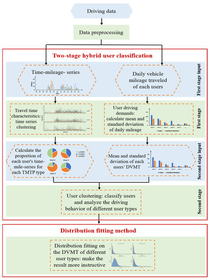
Figure 1.
The overall framework of the driving behavior distribution fitting method.
3.1. Data Collection
The data set used for this study reflects real usage data from traditional private cars, provided by an automobile manufacturer in China. Data acquisition equipment is installed in cars before leaving the factory. Real-time vehicle usage data are subsequently collected every 10 s and transmitted to a server. Regarding study subjects, Beijing users are selected. The data set for this study includes data from 21,490 vehicles, from April 2020 to December 2020. The number of data records per month for each vehicle ranges from 500 to 100,000.
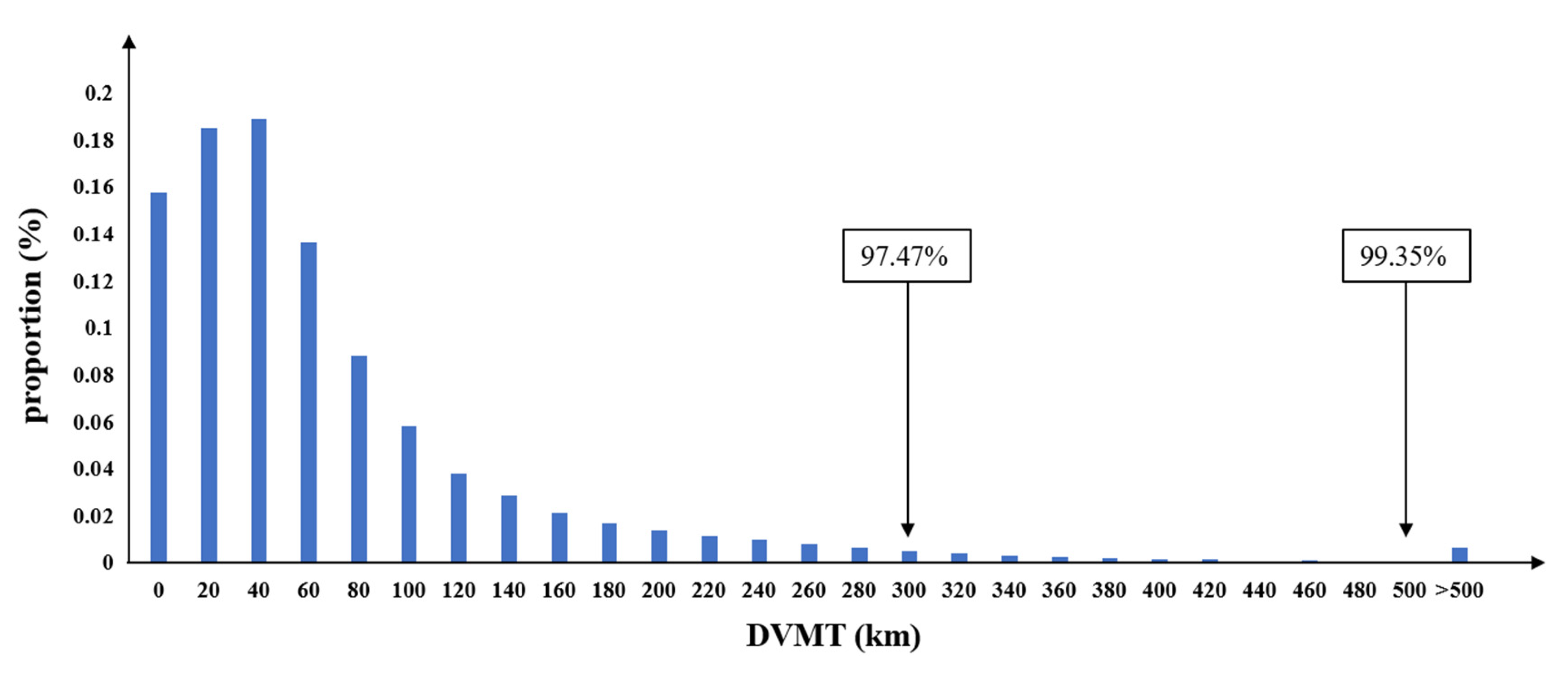
Table 1 describes the data set and indicates that the DVMT of the 1000 vehicles varies significantly, ranging from 0 to 1506 km. The average DVMT is 63.498 km. The fourth column of Table 1 shows that the data set covers a total of 76.12% active days from April 2020 to December 2020. In addition, Figure 2 shows that only 0.65% of the DVMT values extend beyond 500 km, whereas most DVMT values, 97.47%, are within 300 km.

Table 1.
The description of the data set.

Figure 2.
Histogram of the proportion of DVMT.
3.2. Data Preprocessing
Figure 3 shows the approach used to pre-process the data:
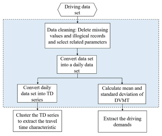
Figure 3.
The data pre-processing approach.
Vehicle driving data usually includes “dirty” data, with missing or illogical values, because of unstable signals or errors in the data transmission process. This makes it necessary to clean the data to improve its quality. First, illogical records and missing values are deleted (for example, as time passes, the total mileage becomes smaller or the vehicle speed suddenly becomes zero). Second, the driving data set includes a total of 244 parameters, including vehicle alarm information, travel information, and key component statuses. However, most of the parameters are null or are unrelated to our experiment. Therefore, we select the data parameters relevant to this experimental research, eliminating unnecessary data parameters to improve experimental efficiency. After data cleaning, 79.64% of the data records remain from the original data, and 7 relevant data parameters are left. Table 2 shows a sample data record.
Table 2.
A sample data record.
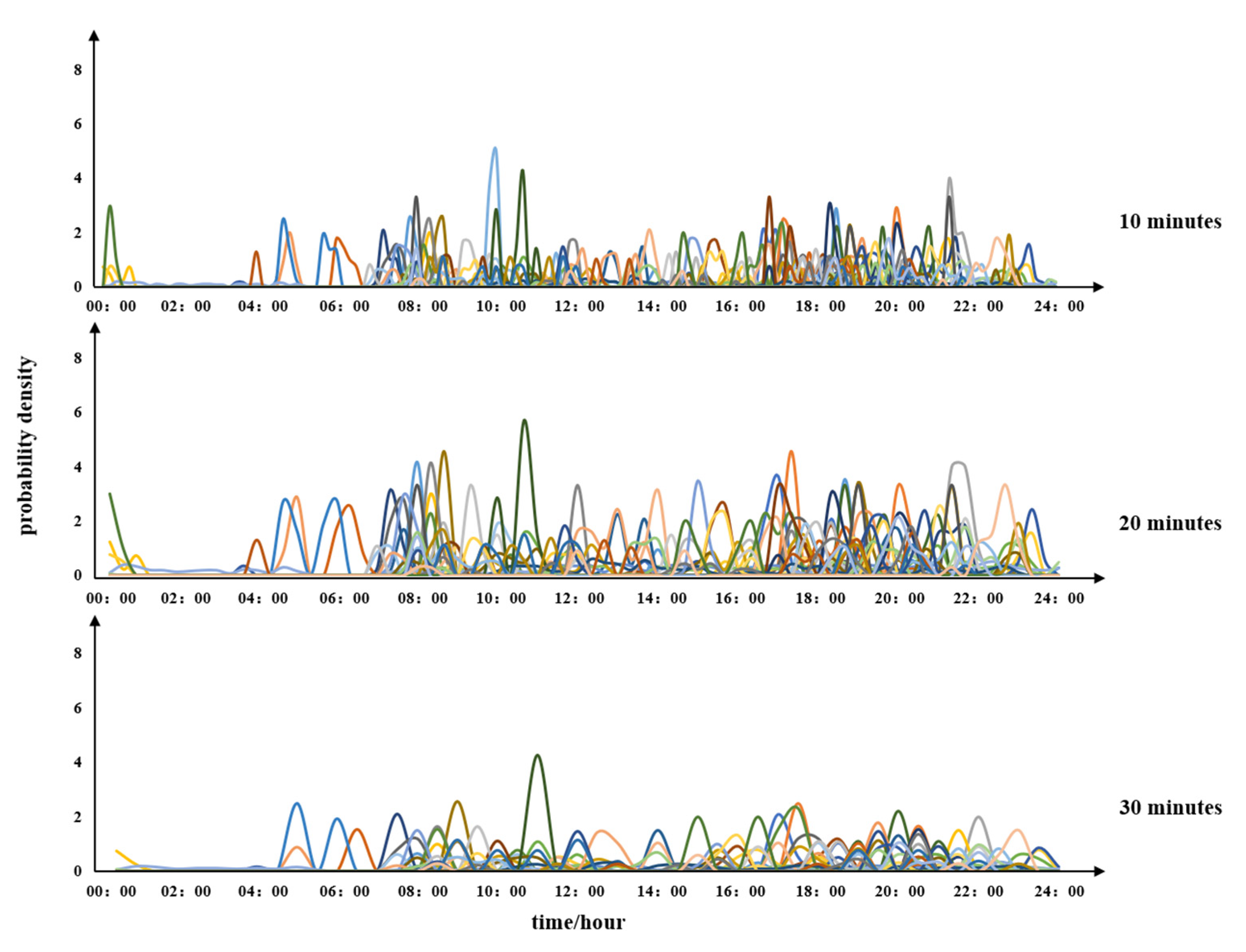
Next, we convert the data records into a daily vector. The data acquisition equipment collected data every 10 s, which is too granular for calculating the time-series and results in excessively long calculation times. However, if the time period used is too long, changes in the time-series may be missed, making the differences difficult to detect. To identify the best unit of time granularity, three kinds of time durations are assessed (10, 20, and 30 min) to observe the patterns in the time-series changes (See Appendix A). A time period of 20 min performs better; as such, 20 min is selected as the recorded value, and the daily vector is converted into a time–mileage-series ().
3.3. Data Analysis: Two-Stage Hybrid User Classification
3.3.1. First Stage: Driving Time Characteristics and User Driving Demands
- 1.
- Driving Time Characteristics: Time-Series Clustering
Different users use a car for different purposes in a given period; that is, the DVMT is usually different. Four users’ DVMT over a week, extracted randomly from our study data, are presented as an example in Figure 4 to describe the difference of vehicle users. The DVMT values of Users 1 and 3 are much larger on the workday compared to the weekend. This is consistent with taxi drivers or long trip travelers. For User 2, the driving behavior is similar to office workers, because of the similarity in the DVMT, demonstrating regular driving behavior. User 4 represents users who use cars mostly on weekends, such as parents taking children on weekend outings. There is a large difference in driving behavior between users. Therefore, to better explain driving behavior, the DVMT of different users is an important part of the experiment.
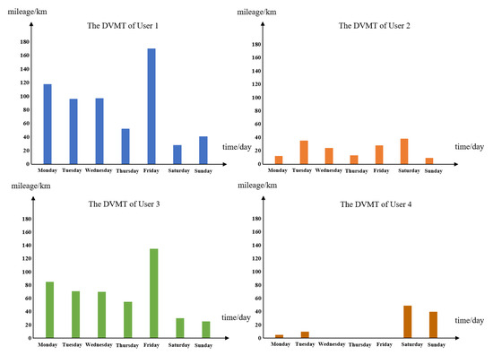
Figure 4.
Examples of DVMT for different users in a week.
In addition, Figure 5 shows that one user had significant diversity in vehicle use, with travel patterns changing on different days. The figure shows the different time–mileage-series patterns of User 1 over a 5-day period (weekdays).
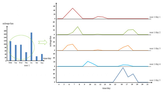
Figure 5.
The time-series distributions for User 1.
Market segmentation and satisfying personalized demands is facilitated by considering the mean and standard deviation of the DVMT, as they reflect the overall trends in each user’s demand. The mean DVMT refers to the user’s average daily vehicle driving mileage, and reflects the central tendency of the overall daily driving distance for each user. The standard deviation of DVMT can reflect the discreteness, or differences, in each user’s driving behavior.
Therefore, this study applies a two-stage hybrid user classification method to classify users. The first step is identifying the typical characteristics of the time-series changes in mileage, that is, the typical daily time–mileage travel patterns (TMTP). This allows the extraction of the typical vehicle usage of all users. Then, the mean and standard deviation of all users are calculated to obtain user driving demands. Finally, based on the distribution of the typical daily TMTP of each user and the mean and standard deviation of all users, the users with similar TMTP distribution and similar travel demands are clustered into individual categories.
The user driving time characteristics are extracted in the first stage. This involves identifying the typical daily time–mileage travel patterns (TMTP) to reflect user driving time characteristics. The time–mileage-series is expressed by the changes of mileage with time . Where denotes the time–mileage-series, and represents the mileage traveled at time . The series is the input of the first stage clustering to get the TMTP centroid.
The K-means algorithm is widely used in studies for clustering, because it is simple in principle, fast in convergence, and strong in interpretability [35]. As such, this study applies the K-means algorithm to cluster time–mileage-series. When using the K-means algorithm for time-series clustering, it is critical to measure the similarity between time series, which is the series.
The Euclidean distance and Dynamic Time Warping (DTW) methods are widely used to measure the similarity of time-series in time-series clustering [36]. Most of the time-series are similar, but out of phase, which means they have different elastic movement on the time axis. For example, Figure 4 shows similar patterns in the time series changes of User 1 on Tuesday and Wednesday. The incomplete time series may be related to the time when the user begins traveling. However, the principle of Euclidean distance is to measure similarity using one-to-one alignment mapping. As such, the Euclidean distance is sensitive to noise and has difficulty capturing dynamic changes, such as time-series translations. Using the Euclidean distance for measurement does not consider the dynamic changes in time, reducing its accuracy.
In contrast, DTW distance allows for elastic movement in the time axis, which can measure the similarity of shape-based time-series [37]. The time-series alignment of DTW is more flexible, and has been widely used to measure the similarities between time-series, replacing the traditional Euclidean distance [36]. Therefore, we use the DTW algorithm to measure the similarity between series.
The process of using the DTW algorithm to measure the similarity between series is as follows.
Set the series , and construct an matrix . Each element in the matrix represents the similarity between each point of the series and each point of the series . The smaller the distance, the higher the similarity. The variable is expressed as:
The curved regular path between the series and the series is expressed as:
The -th element of , . This path must meet the following conditions:
- (1)
- (2)
- For it must meet
To find the curved and regular path between the series and the series , we introduced a time window into the similarity measure. However, if the time window is set to be too large, the difference in the travel patterns in the time period will be significant, resulting in inaccurate results. Therefore, we matched the series and the series in the previous hour and the next hour, as the change of travel patterns for one user in a single hour in different days is very likely to be small.
The cumulative distance is:
The optimal path is the path that minimizes the accumulated distance along the path.
Then, the similarity between the series and the series is the smallest regularization cost between the and the , expressed as :
Clustering the series using the K-means and DTW algorithm generates the class centroid:
- 2.
- User Driving Demands: Daily Vehicle Mileage Traveled (DVMT)
The mean and standard deviation of DVMT of each user reflect the user driving demands, expressed as:
where and refer to the mean and standard deviation of DVMT of -th user, respectively. The variables and refer to the total mileage and total travel days traveled by user during the observation period. The is the DVMT of user traveled on day .
3.3.2. Second Stage: User Clustering
The users with similar TMTP distributions have similar vehicle usage characteristics; as such, they are assumed to have the same travel patterns. Therefore, we introduce the proportion of each vehicle’s series in the class of as a factor for user clustering. Through the first stage of time–mileage-series clustering, we generate the typical , and the type of the series of each vehicle belongs to.
The variable denotes the total number of series of all vehicles; denotes the total number of series of the -th vehicle; and denotes the number of the -th vehicle’s series belonging to the class. Then, the proportion of the series of the -th vehicle belonging to the class is:
Then, the proportion of the series of user is:
However, the typical daily TMTP mainly reflects the distribution of driving time and characteristics. As described in Section 3.3.1, user clustering is needed to consider the mean and standard deviation of DVMT, which are thus introduced as two factors to cluster users.
For user , the driving time characteristics and driving demands can be expressed as:
Then, users with similar characteristics are clustered into one class, based on their driving time characteristics and driving demands (TCDD). The similarity is calculated using the Euclidean distance. This clustering yields user types:
3.4. Distribution Fitting Method
Compared with analyzing the mean and standard deviation of DVMT values, distribution fitting can better explain the driving behavior and have more guiding significance. This is because distribution fitting can display regular user travel patterns and statistically reveal driving habits [25]. Distribution fitting of the DVMT values for different user types can be used in a variety of applications, such as better understanding different user driving behavior, analyzing their travel needs, and providing stronger guidance for the transportation department. Therefore, after obtaining user classes, we performed distribution fitting of the DVMT of these classes.
The Weibull, log-normal, and Gamma distributions are widely used to model and fit right-skewed data [13]. Most scholars use these distributions to study the DVMT of users, rather than normal distribution and Poisson distribution, because they better reflect reality [13]. Reference [38] verified that the log-normal distribution is effective and reliable in fitting the DVMT of vehicles, and has a wide range of applications. Our experimental process found that the three-parameter log-normal distribution, determined by the three parameters , , and , is more suitable for fitting our sample data. Therefore, we select that approach to simulate user DVMT. The probability density function of the three-parameter log-normal distribution is:
4. Result
4.1. First Stage: Driving Time Characteristics and User Driving Demands
4.1.1. Driving Time Characteristics: Time Series Clustering
Using the methods introduced in Section 3.3.1, we performed clustering for , to identify the typical . First, the K-means are applied to cluster the series.
To compare the value, at a time point of one , with the values at that time point in the hour before and after the other s to calculate similarity, the time window was set to 3. After the clustering, all series were divided into classes. However, the selection of significantly impacts clustering performance. When is too large (when the number of classes is too large), there is little significance for clustering; however, having too small a number of classes provides insufficient interpretative value. Therefore, we need to determine the number of classes to achieve a good clustering effect. Figure 6 shows that the clustering performance is better when the number of clustering is six, , that is .
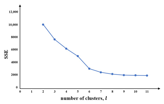
Figure 6.
The SSE index of the time–mileage-series clustering.
This means that the series are divided into six typical daily time–mileage driving patterns (). The sum of the squared errors (SSE) is the core index of the elbow method.
After time series clustering, we randomly selected 100 mileage change patterns from each TMTP types to show the characteristics of different TMTP types, shown in Figure 7. The orange line is the center of the cluster for different TMTP types. The cluster indicates that driving time is mostly concentrated between 7:00–9:00 and 18:00–20:00, with a small concentration at 12:00–13:00. User types can be inferred based on their driving time patterns [3,39]. As such, the driving pattern may reflect the driving behavior of household members going to work and picking up students. The small peak at noon may reflect a drive for lunch. There are two peaks for , at 7:00–9:00 and 17:00–19:00. These correspond to office worker commuting times. For , the DVMT is zero most of the day, indicating infrequent vehicle use. The peaks are at 6:00–7:00 and 16:00–18:00, and the driving distance per unit of time is larger in the afternoon. This may indicate travel patterns for users who use their vehicles infrequently.
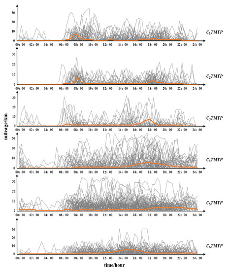
Figure 7.
Typical daily TMDP.
The driving time for is concentrated between 14:00–22:00 and the driving distance per unit of time exceeds other types. It may be that reflects the driving behavior of drivers who frequently go out for entertainment in the afternoon and evening, or drivers working at night. For and , there is no concentrated driving time; users drive their cars from 7:00 to 24:00, indicating they are long-time drivers. In addition, the driving mileage per unit of time of is larger compared to . We can speculate that may reflect the travel patterns of car-sharing drivers or frequent business travelers, whereas the may reflect the travel patterns of an online car hailing driver or taxi driver.
4.1.2. User Driving Demands: Daily Vehicle Mileage Traveled
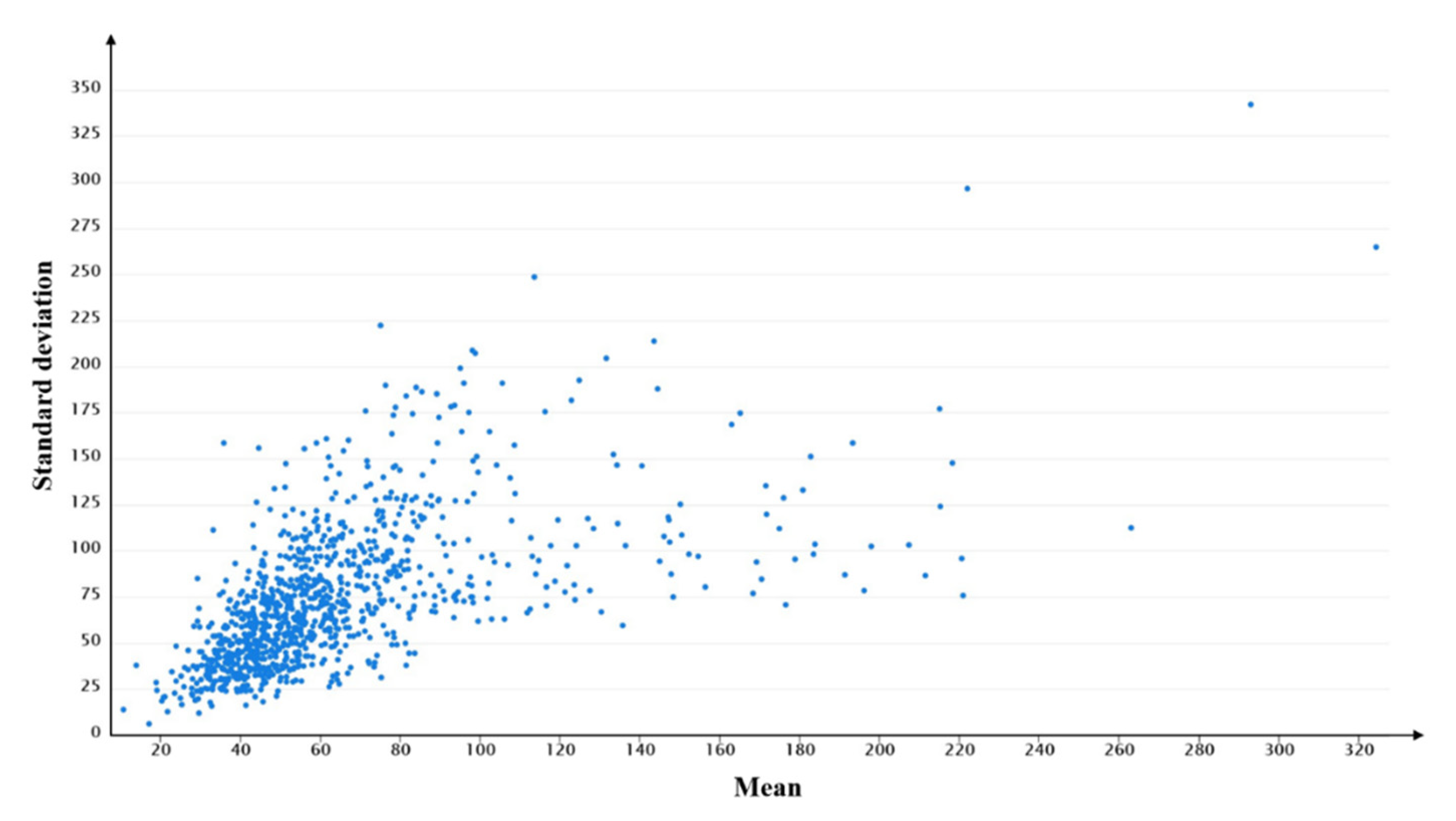
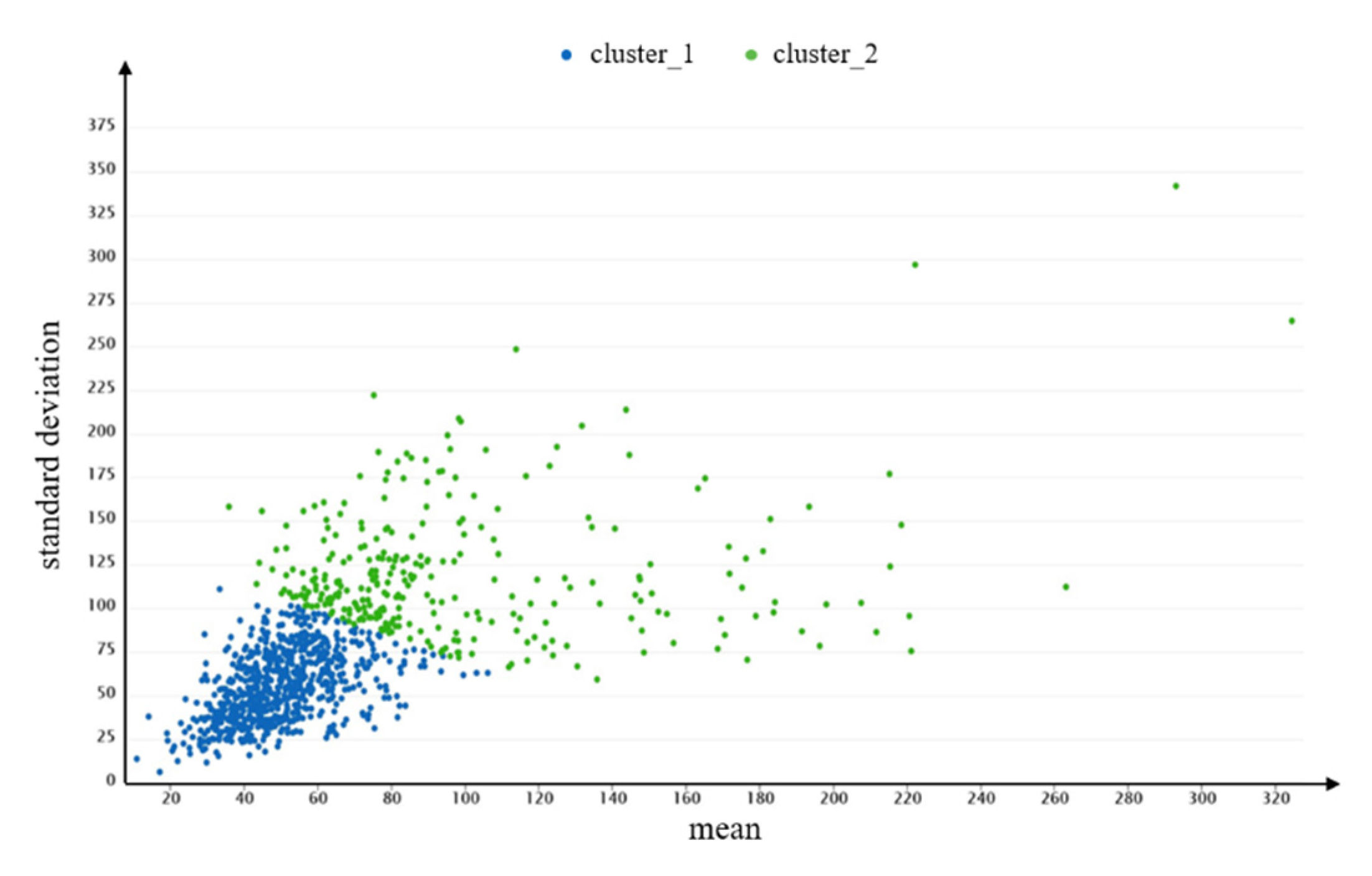
The mean and standard deviation are calculated to show the travel demands and overall tendency of users. Figure 8 shows the distributions of the mean and standard deviation of each users’ DVMT. The mean DVMT value for users ranges from 10.754 to 324.377 km, while the standard deviation of DVMT ranges from 6.293 to 341.996 km. In addition, the average mean and average standard deviation of DVMT of all users are 64.018 and 74.583 km, respectively. The large differences between the mean and the standard deviation of each users’ DVMT indicates that travel demands and the regularity of each user are very different.
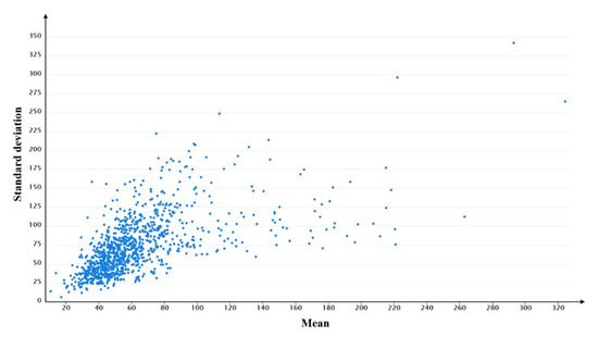
Figure 8.
The distributions of the mean and standard deviation of each users’ DVMT.
4.2. Second Stage: User Clustering
The proportion series of each user are calculated using the method introduced in Section 3.3.1, and the K-means algorithm is used for clustering based on TCDD. Similarly, the number of categories must be determined to achieve a good clustering effect. Table 3 shows the number of clusters and clustering performance. According to the Davies–Bouldin Index (DBI), the performance of four clusters is better than other number of clusters. Therefore, we divided users into four types based on the TCDD, that is .
Table 3.
The number of clusters and clustering performance of TCDD method.
The description of the four user types is shown in Table 4; Figure 9 shows the average proportion of each daily typical TMTP type for each user type. Table 4 shows there are 854 users in user types and , representing 85.4% of all users. The means of these two separate user types are 59.775 and 49.088 km, with standard deviations of 84.141 and 55.112 km, respectively. The mean and standard deviation of the DVMT values were slightly higher for compared to . In addition, , , and each represent a similar proportion of the total, at around 20% of user type . The , accounts for the largest proportion; accounts for the second highest proportion. Combined with the results of TMTP, we can reaffirm that the user types and likely represent office workers. As we all know, the driving behavior of household office workers is different from that of ordinary office workers. In addition to commuting to and from work, they also have some driving behaviors different from those of office workers, such as picking up and seeing off children [26]. The group may refer to household office workers, who go to work and go out with children on holidays or weekends based on their driving time characteristics and driving demands. The travel patterns of the group are most similar commuters. The and users account for only 14.6% of the total count; the mean DVMT values are 164.732 and 104.812 km, respectively; and the standard deviations are 102.465 and 112.663 km, respectively. The mean and standard deviation of DVMT of user types and are far lower compared to user type and , indicating short driving distances and regular driving behavior for and and irregular and long driving distances for user types and . The largest proportion among these six TMTP types in user type is , which refers to the long-distance driving patterns, and is larger than the other five types. This reaffirms that these may refer to the long-distance drivers going to distant destinations within a specified time. For , the proportion of , , and which may refer to the night driving patterns, are larger compared to the other three TMTP types. Therefore, for , this may include nighttime workers and online car hailing drivers, or users who go out for entertainment at night.
Table 4.
The description of each user type divided by TCDD method.
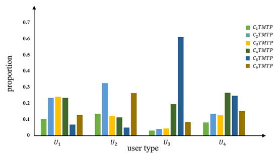
Figure 9.
Average proportion of each TMTP type in U of TCDD method.
The typical daily travel patterns of each user type are analyzed in Section 4.4.
4.3. Distribution Fitting on the DVMT for Different User Types
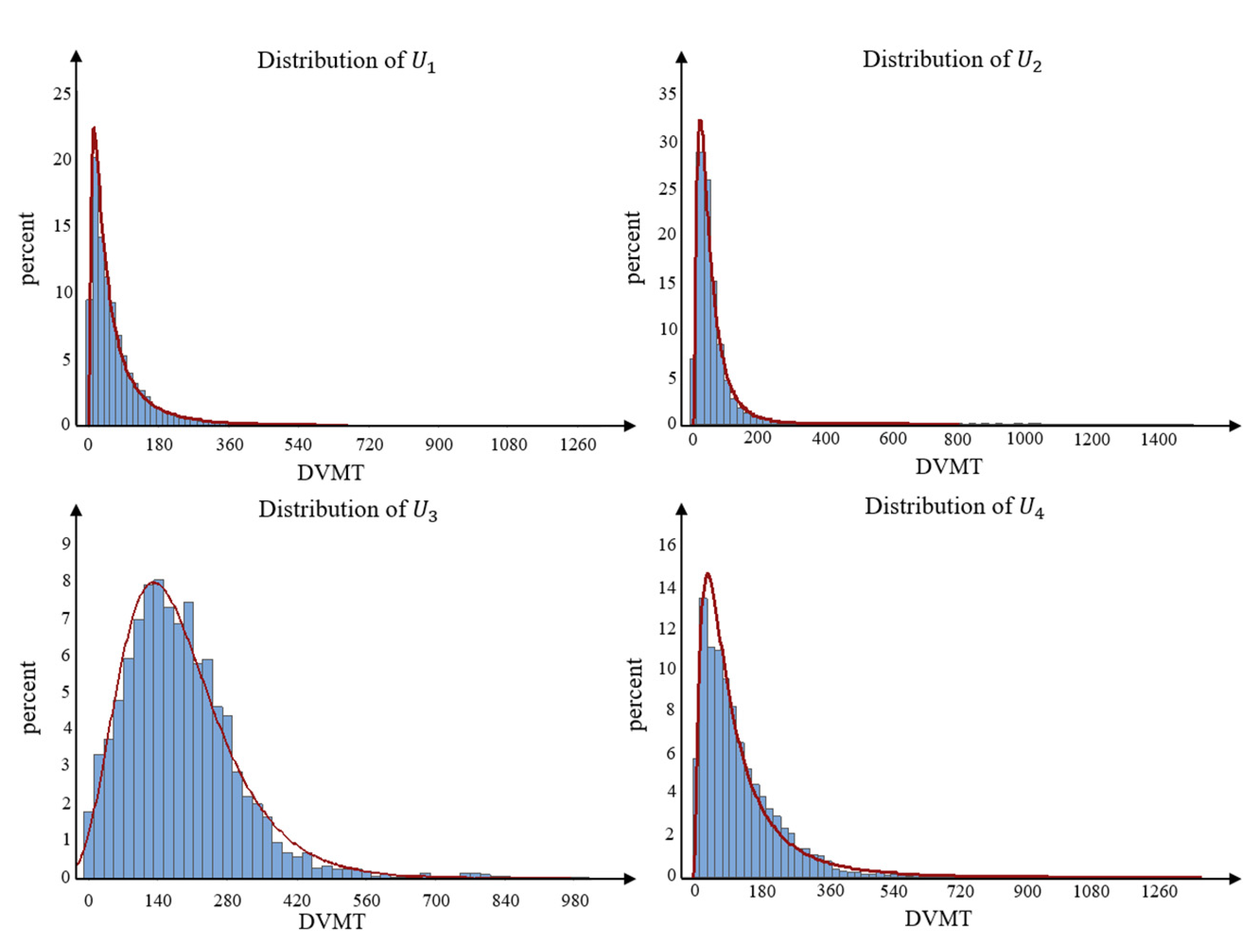
We use the three-parameter log-normal distribution introduced in Section 3.4 to fit the distribution of the values of different user types. The probability density function is expressed in Formula (12). Table 5 shows the fitting results of different parameter values for different user types. The p-value was small in the distribution fitting of different user types. This may be caused by the noise inherent in a large data sample [40]. For example, the smallest number of users among the four user types was 47 users, encompassing 5115 records.
Table 5.
The distribution fitting results.
Figure 10 shows the distribution fitting results of DVMT for different user types. Most DVMT values for user types and are no larger than 400 and 300 km, respectively, accounting for 98.39% and 98.86% of the total observed daily driving patterns, respectively. For user types and , most DVMT values are within 600 km, accounting for 98.89% and 98.72% of the total daily driving patterns. The DVMT values within 50 km of these four user types, , , , and , are 54.10%, 62.87%, 9.07%, and 31.01%, respectively. Most of the DVMT values for users and are between 10 and 50 km. In contrast, for and , the DVMT values are concentrated between 70–250 km and 30–150 km. In addition, the average daily mileage values of user type and exceed those of user type and . This is consistent with the results in Table 4. In contrast with user types and , user types and may be users who drive their vehicles for short distances during most of their driving days. In contrast, user type may refer to long-distance or long-term drivers, who drive vehicles long distances most of their driving days, such as freight drivers. User group may encompass medium and long-distance users.
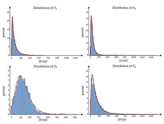
Figure 10.
The results of distribution fitting for different user types.
The distribution fitting results of these four user types help researchers better understand the driving behavior of different users. Enterprises may adopt different marketing strategies for different user groups, based on user type distributions. For example, for people in and , enterprises may market vehicles based on their low fuel consumption and vehicle appearance. This is because most short-distance drivers are likely to drive in urban areas, consuming more fuel each time they accelerate or decelerate. People in and may focus more on performance and vehicle comfort because of the long time spent driving.
4.4. Comparative Analysis
As described in Section 4.1.2, knowing the mean and standard deviation of driver behaviors helps enterprises better meet personalized user demands and improve product quality. However, some studies cluster users based only on the mean and standard deviation of the DVMT [31] (MS-cluster method) and some studies analyze the driving behavior of users by clustering the users according to the proportion of each vehicle’s time series in the TMTP types [37] (TMTP-cluster method). Therefore, experiments were done using two methods to compare the results with this study’s method.
4.4.1. Clustering with the Mean and Standard Deviation (MS-Cluster Method)
The mean DVMT value reflects the central tendency of the overall daily driving distance of each user; the standard deviation of DVMT reflects the discreteness, or differences, of each user’s driving behavior. Therefore, the K-means algorithm cluster users with the two-dimensional Euclidean vector, composed of the mean and standard deviation of each user’s DVMT, to facilitate a comparison of the clustering results with the two-stage hybrid user classification.
After the clustering with the mean and standard deviation, the user types can be expressed as , where refers to the appropriate number of clusters.
The DBI measures clustering performance. Table 6 shows that the DBI is smallest when there are two clusters, indicating that clustering is better when vehicle users are divided into two types according to the mean and standard deviation. Therefore, we divide the users into two types, that is .
Table 6.
The number of clusters and clustering performance of MS-cluster method.
The clustering results are shown in Figure 11 and Table 7. The average mean and standard deviation of DVMT of are smallest; this groups accounts for the largest proportion of total users. The user type may refer to short distance drivers. In contrast, the users of , with the larger mean and standard deviation, may represent the users who drive their vehicles for a long distance in one day.
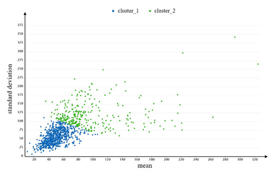
Figure 11.
Clustering results of MS-cluster method.
Table 7.
Clustering results of MS-cluster method.
4.4.2. Clustering with the Proportion of Each Vehicle’s Time Series in the TMTP Types (TMTP-Cluster Method)
As described in Section 3.3.1, users with a similar TMTP can be considered to be the same user type. The K-means algorithm is used to cluster users according to the proportion series for each user calculated in Section 3.3.1. Table 8 shows the clustering results. The DBI index of the TMTP-cluster method indicates that six clusters perform better compared to when a different count of clusters is used. Therefore, we divided users into six types based on the typical daily TMTP, that is, .
Table 8.
The number of clusters and clustering performance of TMTP-cluster method.
There is a total of 838 users in user types , ,, and , accounting for 83.8% of all users. The mean values of , ,, and are 62.710, 72.761, 52.633, and 72.491 km, respectively. The TMTP type accounting for the largest proportion among the six TMTP types of is ; for , the largest is the which is much larger than other types. There appears to be no significant differences between the six TMTP types in user types and . The users of and only account for 16.2%; the mean DVMT values are 165.949 and 102.203 km, respectively, indicating the users may be long-distance drivers. and account for the largest proportion of user type and , respectively. The description of the six user types is shown in Table 9, and the average proportion of each TMTP type in is shown in Figure 12.
Table 9.
The description of each user type divided by TMTP-cluster method.
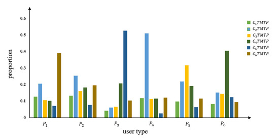
Figure 12.
Average proportion of each TMTP type in P of TMTP-cluster method.
4.4.3. Comparative Results
- (1)
- The Mean and Standard Deviation Distributions of DVMT of Different User Sets
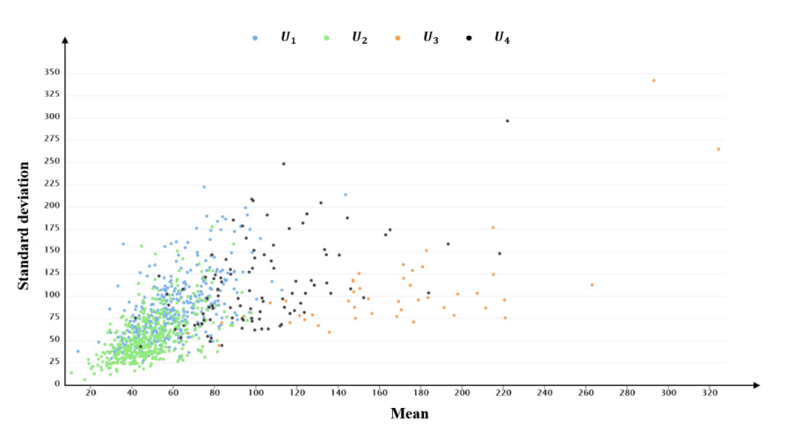
Users are divided into four types, using clustering with the TCDD, and into six types of clustering with the proportion of each vehicle’s time series in the TMTP types. Figure 11, Figure 13 and Figure 14 show the distributions of the mean and standard deviation of DVMT of users divided by these two methods. Figure 14 shows that the distributions of some user types are similar, such as the distributions of and . Table 9 shows that the average mean and standard deviation of user type and are similar with each other. Users are divided into so many groups that the difference between groups is not made clear by using the clustering method with the proportion of each vehicle’s time series in the TMTP types. The discrimination of the mean and standard deviation distributions of user types in user set are better than those in user set . Users are only divided into two types, which do not sufficiently recognize the differences in driving behavior of users. However, the mean and standard deviation distributions in user set are better compared to those in user set and .

Figure 13.
The mean and standard deviation distributions of user set U divided by the TCDD method.
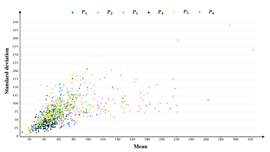
Figure 14.
The mean and standard deviation distributions of P divided by the TMTP-cluster method.
- (2)
- The TMTP Distributions of Different User Types
It would be inaccurate to determine which method is better using only the distribution of the mean and standard deviation of each type of users clustered using different methods. As a reminder, six daily typical TMTP types are obtained in the first stage, representing different travel patterns among the 1000 users. As described in Section 3.3.2, the distribution of the average proportion of different TMTP types in different user types reflects similar vehicle usage patterns; users with similar TMTP distributions are considered to have the same travel patterns. Therefore, it is helpful to compare the methods using the average proportion of different TMTP types in different user sets. Figure 9, Figure 12 and Figure 15 show the average proportion of different TMTP types in user set , user set , and user set , respectively.

Figure 15.
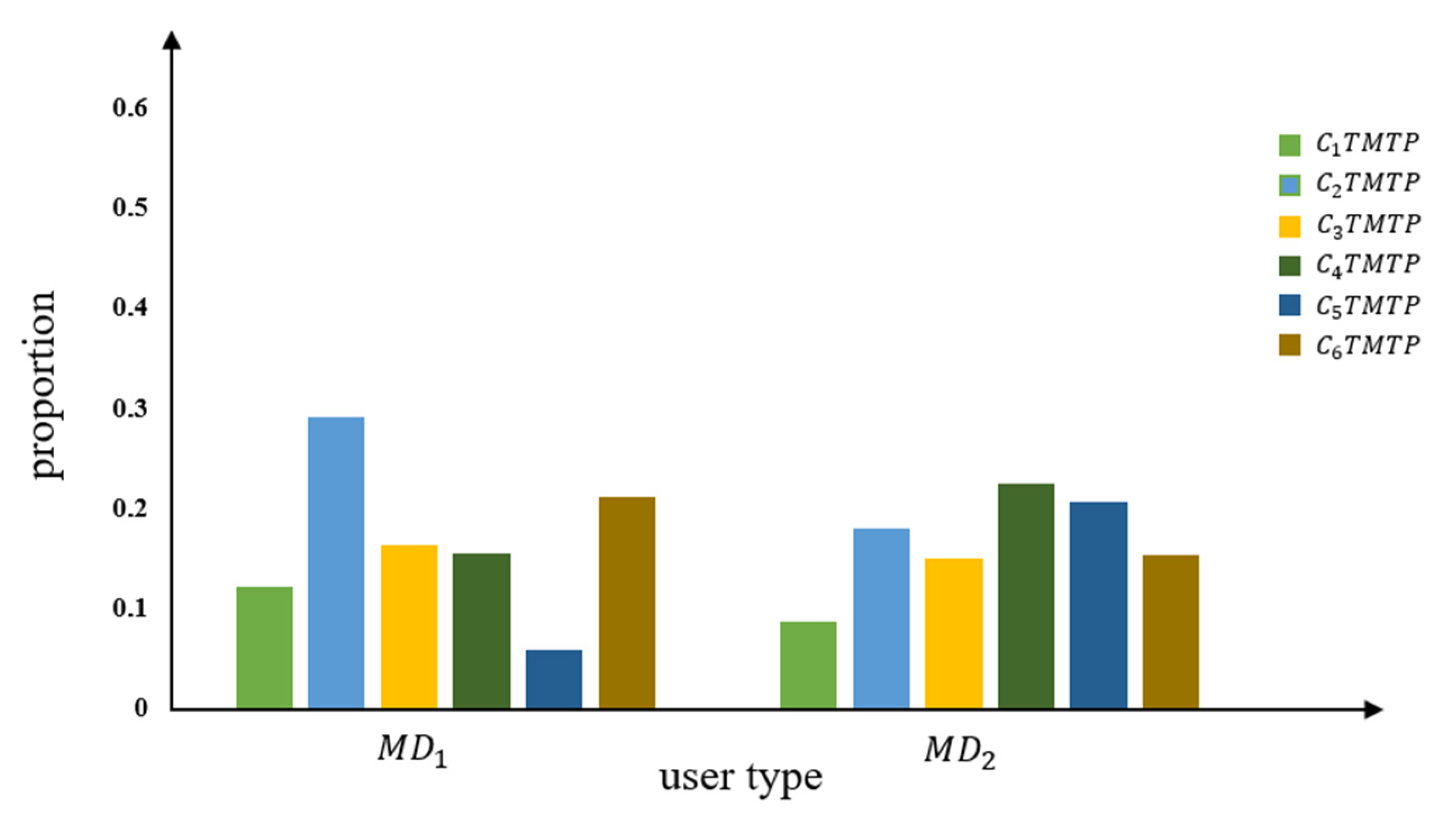
Average proportion of each TMTP type in MD of the MS-cluster method.
For user set , classified using the MS-cluster method, there is no significant difference in the distribution of the average proportion of different TMTP types between user type and . For , there are only small differences among the proportions of different TMTP types in . The largest proportion among the six TMTP types is , accounting for 29% of the total daily driving patterns. The smallest proportion is seen for , accounting for 5%, while the proportions of other TMTP types are similar, around 15%. For , there are only little differences among the proportion of different TMTP types. The proportions of , , and are around 20%, and the proportions of and are around 15%. In summary, there are no clear daily typical TMTP types in user type and , indicating that the MS-cluster method does not effectively distinguish the driving behavior of different users.
For user set , as described in Section 4.1.2 the distributions of TMTP types in each user type differ from each other. For , the proportions of , , and are larger than other three types, and the total proportion of and exceeds 55% in . Combined with the analysis in Section 4.1.2, this indicates that and may refer to office workers. The accounts for 60% of the total daily driving patterns, which is significantly larger compared to other TMTP types in . The represents the driving behavior with long driving distances and night driving, possibly indicating that may refer to the long-distance drivers going somewhere within a set period of time. The proportion of each TMTP type in are similar; however, the total proportion of , , and exceeds 50% in , suggesting this user type may include long-distance drivers or online vehicle hailing drivers.
Compared with the MS-cluster method, the TCDD method better identifies the different driving behavior of different users. The distribution of TMTP differs in different user types. This allows enterprises to adopt different marketing strategies for different user types to meet their personalized needs, based on the TMTP distribution.
Therefore, the TCDD cluster method yields better results than the MS-cluster method and the TMTP-cluster method. The TCDD method divides users into four types; the MS-cluster method yields two user types; and the TMTP-cluster method yields six types. With the TCDD method, the number of user groups is not too small to fully recognize the driving behavior, but there are not so many that it is difficult to distinguish the travel patterns between user types. Accurately and appropriately classifying users helps enterprises better position, improve, and design vehicles based on the driving behavior of different user types, meeting the different demands of user categories.
5. Discussion
Classifying users based on driving time characteristics and user driving demands is important for enterprises and transport departments to better understand users driving behavior. The goal was to propose corresponding measures or policies for users’ driving behavior for different user types.
For enterprises, our method is easy to operate and can provide them with accurate information to segment the market and formulate precise marketing strategies. Different usage patterns and driving demands of vehicle users can be generated through the first stage. Enterprises can design different products or upgrade products or services according to different usage patterns and driving demands, to better meet the differentiated needs of vehicle users. Then, different user types can be obtained by clustering with the driving time characteristics and driving demands through the second stage. Enterprises can conduct market segmentation, precise marketing, and configure products differently for different types of users.
Short-distance drivers, like user types and , usually use their vehicles for commuting, because their driving time is mainly between 7:00–9:00 in the morning and 17:00–19:00 in the afternoon which is consistent with commuting times. Therefore, these users may be more concerned about performance, such as fuel consumption, because high rates of acceleration and deceleration occur due to heavy traffic on the way to and from work. In contrast, user types and may prefer comfortable and high configuration vehicles, even though the cost of these products is higher, because they often drive for a long time and a long distance. Different types of users have different demands for the performance and configuration of vehicle products. As such, enterprises should provide vehicle products with different performance to meet the diverse needs of users, and should conduct targeted marketing strategies for different user types.
Due to environment pollution and the energy shortage crisis, private electric cars and car-sharing electric vehicles have been widely promoted in China [41]. This study’s methods can help enterprises to understand the driving behavior of users, to design the appropriate range of electric vehicles to meet the needs of users. This can also help the government develop targeted electric vehicle policies to boost the spread of electric vehicles and car-sharing electric vehicles.
Our analyses results indicate that user types and are mainly characterized as users who drive at low speeds and over short distances. Enterprises can offer electric cars with small driving ranges to reduce their commuting cost. In contrast, user types and may need electric vehicles that can drive long distance; and generally, the mileage of most electric vehicles on the market can meet most of these driving demands. Enterprises should popularize these electric vehicles with users, to improve their confidence in the mileage of electric vehicles. At the same time, government can improve public charging infrastructure to allow users to charge their cars more conveniently.
The results of this study can also help transport departments develop transport strategies. The results of the driving time characteristics indicate that the peak hours of the driving times are between 7:00–9:00 in the morning and 17:00–20:00 in the afternoon. At the same time, traffic control can be conducted according to users’ driving time characteristics, to reduce traffic jams and traffic pressure. In addition, transport departments can optimize public transport systems and routes to motivate short-distance vehicle drivers to switch to public transport, to reduce environmental pollution and energy consumption.
6. Conclusions
This paper developed a two-stage hybrid user classification method to divide vehicle users into different types, and analyze the driving behavior of those types. This study analyzed real usage data about traditional cars provided by an automobile manufacturer in China. The first stage of the study methods involved time–mileage-series clustering and calculating the mean and standard deviation of DVMT of each user. Time–mileage-series clustering using K-means and DTW algorithm was conducted to identify the typical daily time–mileage travel patterns (TMTP) of all users, while the mean and standard deviation was used to determine travel demands. The second stage of the study methods involved user clustering based on the proportion series of each user and the mean and standard deviation of DVMT (TCDD). After the two-stage hybrid user classification method, four user types were generated. Then, the three-parameter log-normal distribution was used to fit the DVMT distribution of these user types.
A comparative analysis was made to demonstrate the reliability of our clustering method, by clustering the users using the mean and standard deviation of DVMT and clustering using the proportion of each vehicle’s time series in the TMTP types. The comparative analysis shows that the two-stage hybrid user classification method is better than the clustering method with the mean and standard deviation, as well as the clustering method with the proportion of each vehicle’s time series in the TMTP types. The new study approach most effectively distinguishes the driving behavior of different users, the mean and standard deviation distributions of user types, and the distributions of daily travel patterns.
Like most of the studies, this one has some limitations. First, the data set was relatively small, and only covers 9 months of driving. Second, we focused on the DVMT. This omits other factors, such as the driving distance of a single trip, the number of trips in one day, and the traffic conditions. Third, the driving data we used were for private vehicles; we did not analyze differences in driving behavior between private and business vehicle users. Due to data set limitations, we did not analyze the influence of different social demographics, such as city, gender, and age, on users’ driving behavior and the reasons for such influence. Further studies should extend the driving data set and apply this study’s methods using additional driving behavior factors. In addition, the different driving behaviors between private and business vehicle users and user types with different social demographics should be explored in further studies. Despite these limitations, this study expands the scope of research on traditional vehicle driving demands and driving patterns by providing a classification method that can combine the user’s daily driving patterns and travel demands. This makes the results more widely applicable compared to methods that only consider driving patterns or driving demands.
Author Contributions
Conceptualization, H.S., Q.Z., and W.W.; methodology, Q.Z.; software, Q.Z.; validation, H.S. and X.T.; formal analysis, X.T.; investigation, X.T.; resources, H.S.; data curation, H.S.; writing—original draft preparation, Q.Z. and W.W.; writing—review and editing, H.S. and X.T.; visualization, Q.Z.; supervision, X.T.; project administration, H.S. All authors have read and agreed to the published version of the manuscript.
Funding
This research was funded by the Fundamental Research Funds for the Central Universities (No. JZ2020HGQA0168).
Conflicts of Interest
The authors declare no conflict of interest.
Abbreviations
| DVMT | Daily vehicle mileage traveled |
| TMTP | Time–mileage travel patterns |
| DTW | Dynamic Time Warping |
| TD | Time–mileage-series |
| PD | probability density |
| C | The set of typical TMTP |
| TCDD | The method of clustering based on driving time characteristics and driving demands of users |
| U | The user set clustering based on TCDD method |
| MS-cluster | Clustering with the mean and standard deviation |
| MD | The user set clustering based on MS-cluster method |
| TMTP-cluster | Clustering with the proportion of each vehicle’s time series in the TMTP types |
| P | The user set clustering based on TMTP-cluster method |
Appendix A. The Appropriate Time Granularity
To identify the best time period granularity, three kinds of time durations are assessed (10 min, 20 min, 30 min) to observe the patterns in the time-series changes. Figure A1 shows that the daily vector is converted into time–mileage-series ; 50 series are randomly selected to determine the optimal granularity of the time period duration. The probability density (PD) at time refers to the value that is 10 times the ratio of the driving mileage at to the daily total driving mileage. The characteristics of the series cannot be sufficiently distinguished at a time granularity of 10 min; thus, the typical daily driving patterns (TMTP) cannot be effectively explained. However, a 30 min time period duration is too large, missing smaller duration trips and inadequately reflecting the real user travel patterns. Figure A1 shows that a time period of 20 min performs better, with more interpretable series results. Therefore, 20 min is selected as the recorded value.
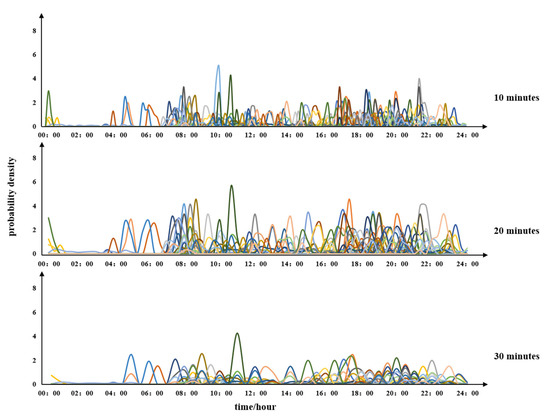
Figure A1.
series of different time period durations.
References
- Lin, B.; Wu, W. The impact of electric vehicle penetration: A recursive dynamic CGE analysis of China. Energy Econ. 2021, 94, 105086. [Google Scholar] [CrossRef]
- Chen, H.; Yang, C.; Xu, X. Clustering Vehicle Temporal and Spatial Travel Behavior Using License Plate Recognition Data. J. Adv. Transp. 2017, 2017, 1738085. [Google Scholar] [CrossRef]
- Zhao, Y.; Zhu, X.; Guo, W.; She, B.; Yue, H.; Li, M. Exploring the Weekly Travel Patterns of Private Vehicles Using Automatic Vehicle Identification Data: A Case Study of Wuhan, China. Sustainability 2019, 11, 6152. [Google Scholar] [CrossRef] [Green Version]
- Bansal, P.; Kockelman, K.M.; Schievelbein, W.; Schauer-West, S. Indian vehicle ownership and travel behavior: A case study of Bengaluru, Delhi and Kolkata. Res. Transp. Econ. 2018, 71, 2–8. [Google Scholar] [CrossRef]
- McNerney, J.; Needell, Z.A.; Chang, M.T.; Miotti, M.; Trancik, J.E. TripEnergy: Estimating Personal Vehicle Energy Consumption Given Limited Travel Survey Data. Transp. Res. Rec. J. Transp. Res. Board 2017, 2628, 58–66. [Google Scholar] [CrossRef] [Green Version]
- Tsai, Y.-C.; Lee, W.-H.; Chou, C.-M. A safety driving assistance system by integrating in-vehicle dynamics and real-time traffic information. In Proceedings of the 2017 IEEE 8th International Conference on Awareness Science and Technology (iCAST), Taichung, Taiwan, 8–10 November 2017; pp. 416–421. [Google Scholar] [CrossRef]
- Chen, C.; Zhao, X.; Yao, Y.; Zhang, Y.; Rong, J.; Liu, X. Driver’s Eco-Driving Behavior Evaluation Modeling Based on Driving Events. J. Adv. Transp. 2018, 2018, e9530470. [Google Scholar] [CrossRef] [Green Version]
- Hsu, C.-Y.; Lim, S.S.; Yang, C.-S. Data mining for enhanced driving effectiveness: An eco-driving behaviour analysis model for better driving decisions. Int. J. Prod. Res. 2017, 55, 7096–7109. [Google Scholar] [CrossRef]
- Charlton, J.; Koppel, S.; D’Elia, A.; Hua, P.; Louis, R.S.; Darzins, P.; Di Stefano, M.; Odell, M.; Porter, M.; Myers, A.; et al. Changes in driving patterns of older Australians: Findings from the Candrive/Ozcandrive cohort study. Saf. Sci. 2019, 119, 219–226. [Google Scholar] [CrossRef]
- Kaneko, M.; Kagawa, S. Driving propensity and vehicle lifetime mileage: A quantile regression approach. J. Environ. Manag. 2021, 278, 111499. [Google Scholar] [CrossRef] [PubMed]
- Wang, H.; Zhang, X.; Wu, L.; Hou, C.; Gong, H.; Zhang, Q.; Ouyang, M. Beijing passenger car travel survey: Implications for alternative fuel vehicle deployment. Mitig. Adapt. Strat. Glob. Chang. 2014, 20, 817–835. [Google Scholar] [CrossRef]
- Dissanayake, D.; Morikawa, T. Household Travel Behavior in Developing Countries: Nested Logit Model of Vehicle Ownership, Mode Choice, and Trip Chaining. Transp. Res. Rec. J. Transp. Res. Board 2002, 1805, 45–52. [Google Scholar] [CrossRef] [Green Version]
- Plötz, P.; Jakobsson, N.; Sprei, F. On the distribution of individual daily driving distances. Transp. Res. Part B Methodol. 2017, 101, 213–227. [Google Scholar] [CrossRef]
- Lin, Z.; Dong, J.; Liu, C.; Greene, D. PHEV Energy Use Estimation: Validating the Gamma Distribution for Representing the Random Daily Driving Distance. In Proceedings of the Transportation Research Board 91st Annual Meeting, Washington, DC, USA, 22–26 January 2012. [Google Scholar]
- Chen, J.; Cai, B.; ShangGuan, W.; Wang, J. Influence of vehicle cluster driving behavior on traffic flow efficiency. In Proceedings of the 2017 Chinese Automation Congress (CAC), Jinan, China, 20–22 October 2017; pp. 6349–6354. [Google Scholar] [CrossRef]
- Wu, Q.; Lan, R.; Zhou, W. Traffic Flow Simulation Based on Adaptive Agent. In Proceedings of the 2018 3rd International Conference on Smart City and Systems Engineering (ICSCSE), Xiamen, China, 29–30 December 2018; pp. 697–700. [Google Scholar] [CrossRef]
- Yang, L.; Wang, X. Clustering of Freight Vehicle Driving Behavior Based on Vehicle Networking Data Mining; Frontier Computing: Singapore, 2018; pp. 12–23. [Google Scholar] [CrossRef]
- Ping, P.; Qin, W.; Xu, Y.; Miyajima, C.; Takeda, K. Impact of Driver Behavior on Fuel Consumption: Classification, Evaluation and Prediction Using Machine Learning. IEEE Access 2019, 7, 78515–78532. [Google Scholar] [CrossRef]
- Michelle, I. The Effects of Driving Style and Vehicle Performance on the Real-World Fuel Consumption of U.S. Light-Duty Vehicles; Massachusetts Institute of Technology: Cambridge, MA, USA, 2010. [Google Scholar]
- Han, T.; Jing, J.; Özgüner, Ü. Driving Intention Recognition and Lane Change Prediction on the Highway. In Proceedings of the 2019 IEEE Intelligent Vehicles Symposium (IV), Paris, France, 9–12 June 2019; pp. 957–962. [Google Scholar] [CrossRef] [Green Version]
- Zhang, J.; Yan, J.; Liu, Y.; Zhang, H.; Lv, G. Daily electric vehicle charging load profiles considering demographics of vehicle users. Appl. Energy 2020, 274, 115063. [Google Scholar] [CrossRef]
- Yun, D.S.; Kim, D.H.; Kim, K.-H. A Study on the Change of the Fuel Efficiency based on the Driving Pattern. J. Converg. Inf. Technol. 2013, 8, 787–794. [Google Scholar] [CrossRef]
- Langbroek, J.H.; Franklin, J.P.; Susilo, Y.O. Electric vehicle users and their travel patterns in Greater Stockholm. Transp. Res. Part D Transp. Environ. 2017, 52, 98–111. [Google Scholar] [CrossRef]
- Zhang, X.; Zou, Y.; Fan, J.; Guo, H. Usage pattern analysis of Beijing private electric vehicles based on real-world data. Energy 2019, 167, 1074–1085. [Google Scholar] [CrossRef]
- He, J.; Yamamoto, T.; Miwa, T.; Morikawa, T. Hazard Duration Model with Panel Data for Daily Car Travel Distance: A Toyota City Case Study. Sustainability. 2020, 12, 6331. [Google Scholar] [CrossRef]
- Khayati, Y.; Kang, J.E. Comprehensive scenario analysis of household use of battery electric vehicles. Int. J. Sustain. Transp. 2019, 14, 85–100. [Google Scholar] [CrossRef]
- Jensen, A.F.; Mabit, S.L. The use of electric vehicles: A case study on adding an electric car to a household. Transp. Res. Part A Policy Pract. 2017, 106, 89–99. [Google Scholar] [CrossRef] [Green Version]
- De Cauwer, D.C.; Gillis, T.C.; Van Mierlo, J. Identification of EV use patterns, based on large scale EV monitoring data. In Proceedings of the 2013 World Electric Vehicle Symposium and Exhibition (EVS27), Barcelona, Spain, 17–20 November 2013; pp. 1–11. [Google Scholar] [CrossRef] [Green Version]
- Greene, D.L. Estimating daily vehicle usage distributions and the implications for limited-range vehicles. Transp. Res. Part B Methodol. 1985, 19, 347–358. [Google Scholar] [CrossRef]
- Smith, R.; Shahidinejad, S.; Blair, D.; Bibeau, E. Characterization of urban commuter driving profiles to optimize battery size in light-duty plug-in electric vehicles. Transp. Res. Part D Transp. Environ. 2011, 16, 218–224. [Google Scholar] [CrossRef]
- Pearre, N.S.; Kempton, W.; Guensler, R.L.; Elango, V.V. Electric vehicles: How much range is required for a day’s driving? Transp. Res. Part C Emerg. Technol. 2011, 19, 1171–1184. [Google Scholar] [CrossRef]
- Tamor, M.A.; Gearhart, C.; Soto, C. A statistical approach to estimating acceptance of electric vehicles and electrification of personal transportation. Transp. Res. Part C Emerg. Technol. 2013, 26, 125–134. [Google Scholar] [CrossRef]
- Khan, M.; Machemehl, R. Commercial vehicles time of day choice behavior in urban areas. Transp. Res. Part A Policy Pract. 2017, 102, 68–83. [Google Scholar] [CrossRef]
- Yang, J.; Liu, A.A.; Qin, P.; Linn, J. The effect of vehicle ownership restrictions on travel behavior: Evidence from the Beijing license plate lottery. J. Environ. Econ. Manag. 2020, 99, 102269. [Google Scholar] [CrossRef]
- Zhao, X.; Yu, Q.; Ma, J.; Wu, Y.; Yu, M.; Ye, Y. Development of a Representative EV Urban Driving Cycle Based on a k-Means and SVM Hybrid Clustering Algorithm. J. Adv. Transp. 2018, 2018, e1890753. [Google Scholar] [CrossRef]
- Anh, D.T.; Thanh, L.H. An efficient implementation of k-means clustering for time series data with DTW distance. Int. J. Bus. Intell. Data Min. 2015, 10, 213. [Google Scholar] [CrossRef]
- Li, X.; Zhang, Q.; Peng, Z.; Wang, A.; Wang, W. A data-driven two-level clustering model for driving pattern analysis of electric vehicles and a case study. J. Clean. Prod. 2019, 206, 827–837. [Google Scholar] [CrossRef]
- Plötz, P.; Gnann, T.; Wietschel, M. Total ownership cost projection for the German electric vehicle market with implications for its future power and electricity demand. In Proceedings of the 7th Conference on Energy Economics and Technology Infrastructure for the Energy Transformation, Perth, Australia, 24–27 June 2012; Volume 27. [Google Scholar]
- Lou, J.; Cheng, A. Detecting Pattern Changes in Individual Travel Behavior from Vehicle GPS/GNSS Data. Sensors 2020, 20, 2295. [Google Scholar] [CrossRef]
- Khoo, Y.B.; Wang, C.-H.; Paevere, P.; Higgins, A. Statistical modeling of Electric Vehicle electricity consumption in the Victorian EV Trial, Australia. Transp. Res. Part D Transp. Environ. 2014, 32, 263–277. [Google Scholar] [CrossRef]
- Wang, Y.; Zhang, N.; Zhuo, Z.; Kang, C.; Kirschen, D. Mixed-integer linear programming-based optimal configuration planning for energy hub: Starting from scratch. Appl. Energy 2018, 210, 1141–1150. [Google Scholar] [CrossRef]


Publisher’s Note: MDPI stays neutral with regard to jurisdictional claims in published maps and institutional affiliations. |
© 2021 by the authors. Licensee MDPI, Basel, Switzerland. This article is an open access article distributed under the terms and conditions of the Creative Commons Attribution (CC BY) license (https://creativecommons.org/licenses/by/4.0/).