Time Distribution Simulation of Household Power Load Based on Travel Chains and Monte Carlo–A Study of Beijing in Summer

Abstract

In recent years, China’s residential electricity consumption has continued to grow at high speed, and its contribution to the growth of the total electricity consumption has become more prominent. The peak-to-valley gap is also gradually increasing, which reduces the efficiency of electricity—an increasingly important terminal energy form. The resident travel chain is a major influencing factor of residents’ electricity consumption, and it is of great significance to dig deeper into the mechanism of its influence on residents’ electricity consumption behavior. In this paper, the time distribution model of household power load in summer in Beijing is constructed by comprehensively considering the difference of travel chain, electricity consumption behavior, and load level. The Monte Carlo simulation method is introduced for the simulation of the model. According to the results, both household type and temperature have a significant impact on the peak load, while the difference in the choice of mode of transportations does not. It is also found that the household appliance with the most potential for regulation is the air conditioning, followed by the water heater, which where regulation and optimization should be mainly carried out.

1. Introduction

In recent years, with China’s social and economic development and the improvement of people’s living standards, residential electricity consumption (REC) has become an important part of the electricity consumption of the entire society, accounting for 14%, and it has shown a trend of rapid growth, exceeding the growth rate of the whole social electricity consumption in the same period. As a representative of megacities, Beijing has a relatively small residential electricity consumption unit, but the overall level of total electricity consumption is relatively high. With the elimination and control of high energy-consuming and high-polluting enterprises in recent years, residential electricity consumption accounted for a large proportion of the total regional electricity consumption, reaching more than 22% in 2018, far exceeding the national level during the same period, and its growth rate is also very considerable. The average growth rate in the five- year period from 2014 to 2018 reached more than 10%. In 2018, the single-year growth rate even exceeded 18%. It can be seen that the level of electricity consumption and growth rate of Beijing residents are at a relatively high level.

While bringing convenience to residents’ life, inappropriate electricity use will also have an impact on the environment. Therefore, energy policies are needed to induce the efficient use of electricity in the residential sector. The analysis of the influence mechanism of residential electricity consumption is important basic work in order to do a good job in the sustainable development of power supply. The purpose is to fully understand the law and difference of residential electricity consumption behavior, and to provide personalized and differentiated service for users while serving the operation of the power system. At present, some scholars have carried out related research on the influence mechanism of residential electricity consumption, mainly including the analysis of influencing factors and behavior analysis.

Traditional factor analysis of microscopic residential electricity is limited by the difficulty of acquiring high-resolution data. Most research involves qualitative analysis and quantitative analysis at the macro level. With the promotion and popularization of smart meters in the residents’ side, the automatic measurement, data processing, and two-way communication ability enables scholars to analyze the influencing factors of residential electricity consumption from the perspective of micro households and present diversified conclusions. Huang [1] used the logarithmic mean Divisia index method (LMDI) to break down the electricity consumption of Taiwan residents based on the data from a questionnaire survey of 7677 households. It was found that climate and the number of households were the first and second major factors driving the growth of residential electricity consumption. Based on the load data of power grid companies and household-related information obtained from mail surveys, Kavousian et al. [2] found that weather, house location, and building area are the most important determinants of residential electricity consumption through factor analysis and stepwise regression analysis. Zheng et al. [3] found that the number of days of cool weather in Guangzhou, China, is significantly related to electricity consumption. Some researchers used a number of downscaling climate models to obtain the stable sequence of daily average temperature and maximum temperature. Regression analysis was used to construct the temperature–power response function of daily residential electricity consumption and daily average temperature, laying a foundation for long-term residential electricity consumption prediction [4,5,6]. Frondel et al. [7] combined the conditional demand method with the quantile regression method to estimate the contribution of common household appliances to electricity demand. It was found that households with relatively low consumption tend to consume electricity to obtain more basic services, such as cooling and hot water. Craig [8] analyzed the relationship between climate change and household electricity consumption and proposed the influence of positive consumer cognition on energy efficiency. Auffhammer [9] used the logistic diffusion model to find that income growth was the main reason for stimulating the consumption of household appliances in rural China. Martinsson et al. [10] conducted a survey in Sweden, and compared the different influences of energy conservation, environmental protection, and low-carbon life attitude of high-income and low-income households on household electricity consumption. Yalcintas and Kaya [11] checked the impact of each factor on residential electricity consumption in Hawaii through linear regression and found that there was a certain degree of negative correlation between average household size and average household electricity consumption. Chen [12] examined the factors affecting residential electricity consumption through two approaches. The analysis reveals that GDP keeps a high relationship with the installation of electrical appliances and eventually leads to an increase in residential electricity consumption. Permana et al. [13] found that when the energy consumption and control in a household were completely decided by women, the energy consumption was always the lowest, through questionnaire survey and face-to-face interview, while the study of Xu et al. [14] believed that there was no obvious relationship between gender and electricity consumption.

With the deepening of smart grid construction, smart meters, smart switches, and other advanced equipment have gradually become popularized. The application of advanced big data, intelligent equipment, and communication measurement technology to carry out residential electricity behavior analysis has become the mainstream. Zhou and Yang [15] propose that changing household energy consumption behavior can effectively improve energy efficiency and promote energy conservation and emission reduction. Hossein [16] regarded electricity consumption as the result of housing selection behavior. By constructing Interpretative Structure Modeling, Hossein established the relationship between behavior characteristics and building characteristics, and analyzed the relationship between household attributes, travel conditions, building attributes, and household energy consumption. Pan et al. [17] extracted residential power load patterns with standard k-means clustering method and classified residents according to age, income, and seasonal power load patterns. Hino et al. [18] used Gaussian mixture model to carry out cluster analysis and effectively extracted the typical electricity consumption patterns of users. Mamchych and Wallin [19] defined the calculation method of multi-day power load correlation between two households and used K-means to conduct cluster analysis on the 28-day load data of each sample household. The results showed that the sample distribution of households with higher self-correlation was relatively dispersed after clustering. Wen et al. [20] proposed a shape-based clustering method for recognizing typical electricity consumption patterns and verified it with data from Ireland and Jiangsu, China, respectively. Wang et al. [21] used a clustering method to classify the household electricity consumption pattern (ECP), and an improved Apriori algorithm was proposed to reveal the relationship between household ECP and residential, social population, and other characteristics. It was found that sociodemographic (except gender) and cooking-related factors such as employment status and whether the occupant used electricity for cooking had significant effects on ECPs, while attitude-related factors had little effect on ECPs.

Based on the summary of the above-mentioned related research, it has been found that the related research on influencing factors seldom consider the influence on the load curve, and fails to take into account the residents’ travel chain, which is an important factor affecting the distribution of household power load (HPL).

Since most of the household electrical appliances are usually interrupted when residents are not at home, the time distribution of HPL is greatly affected by the travel chain. With the advancement of social and economic development and urbanization, in today’s large and medium-sized cities, the residents’ travel chain increasingly has obvious rules to follow, showing the distinctive characteristics of morning and evening peaks during working days. As a representative of mega-cities, Beijing has an obvious trend of double peak of residents’ travel in the morning and evening. In 2018, the travels during the morning peak period from 7:00 to 9:00 accounted for 32.7% of the total daily travels, and those during the evening peak period from 17:00 to 19:00 accounted for 20.8% of the total daily travels [22].

Therefore, it is of great significance to study the time distribution of HPL through the travel chain. The research on HPL from the perspective of the travel chain can help us better understand the mechanism of HPL affected by residents’ behavior, which is basic research that plays an important role in supporting the clean and efficient utilization of electric energy in the department of residents. This paper innovatively puts forward a method to study the distribution of residential power load through the residents’ travel chain, which allows us to learn about the mechanism of household electricity consumption from another angle. By comparing the simulation results with load curves of a community in Beijing, the validation of the model is verified. According to the results, both household type and temperature have a significant impact on the peak load, while the difference in the choice of mode of transportations does not. It is also found that the household appliance with the most potential for regulation is the air conditioning, followed by the water heater, where the regulation and optimization should be mainly carried out.

2. Materials and Methods

2.1. Monte Carlo Simulation

Monte Carlo Simulation was developed from the Manhattan Project of the United States in 1940s. It is a numerical method based on random experiment and statistical calculation, also known as computer stochastic simulation method or statistical simulation method. The mathematical basis of the Monte Carlo simulation method is the law of large numbers and the central limit theorem in probability theory. By linking the solved problem with a certain probability model, the random number generated by the computer is used to realize statistical simulation or sampling, so as to obtain the approximate solution of the problem. Compared with other numerical methods, the Monte Carlo method easily deals with high-dimensional problems. The complexity and computational requirements usually increase linearly as the dimension increases. Considering the randomness of residents’ travel and electricity consumption behavior and the complexity of the interaction among many random factors, the Monte Carlo simulation method is more suitable for the application scenario of this paper.

The steps of the Monte Carlo method are (1) construct probabilistic models of real problems; (2) according to the characteristics of the probability model, design and use various methods to reduce the variance and accelerate the convergence of the test; (3) give the sampling methods of random variables with different distributions in the probabilistic model; and (4) count the results of the experiment and give the solution and precision estimation of the problem.

In the following section, based on the theoretical basis of the Monte Carlo method, the random sampling method of residential travel chain, the generation method of household power load, and the simulation process were respectively carried out, and the time distribution of household power load in summer of Beijing was simulated and analyzed.

2.2. Simulation Analysis of Residential Power Load Characteristics Based on Travel Chains

This section first builds a travel chain model for Beijing residents based on the statistical analysis of the five main characteristics of Beijing residents, including mode of transportation, travel time, time consumption of travel, travel destination, and length of stay at destination.

Next, the households were divided into 5 types, and the electricity consumption period of the day was divided into 6 parts. Referring to the power of common household appliances, the household power load level under different periods of time was constructed.

Then, the Monte Carlo simulation algorithm was adopted. Based on the two models above, the characteristics of Beijing residents’ travel chain in summer were taken as the parameters that were input into the model. The aggregate load curve and average load curve of all kinds of families were obtained by generating travel chain and then load curves.

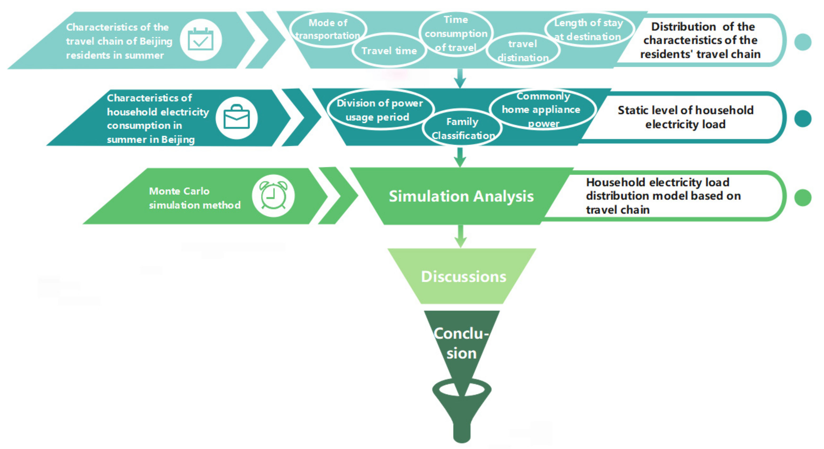
Finally, according to the load curves obtained by simulation, the electricity consumption characteristics of various residents were analyzed, and targeted suggestions for regulation were given. The technology roadmap for this article is shown in Figure 1.

2.2.1. Characteristics of the Travel Chain of Beijing Residents

The travel chain is a process in which individuals, in order to complete one or more activities, start from the starting point at a certain time, pass through several destinations in a certain order through a certain mode of transportation, and finally reach the destination to complete the journey. A travel chain has the following six basic characteristics: Travel starting point, mode of transportation, travel time, time consumption of travel, travel destination, and length of stay at destination, represented by symbols s, a, b, c, d, and e. These characteristics can accurately describe the process of a resident’s travel. Each of these factors can affect the behavior of residents’ electricity consumption by influencing the travel chain. Therefore, the six factors are indispensable in the model.

There are many categories of travel chains. According to the scope of travel, they can be divided into urban travel chains and intercity travel chains. Furthermore, there is a big difference between the travel of working days and the travel of weekends. For ease of discussion, the urban travel chain of only working days is analyzed, and the corresponding travel chain is constructed with the residential area as the starting point.

Mode of Transportation a

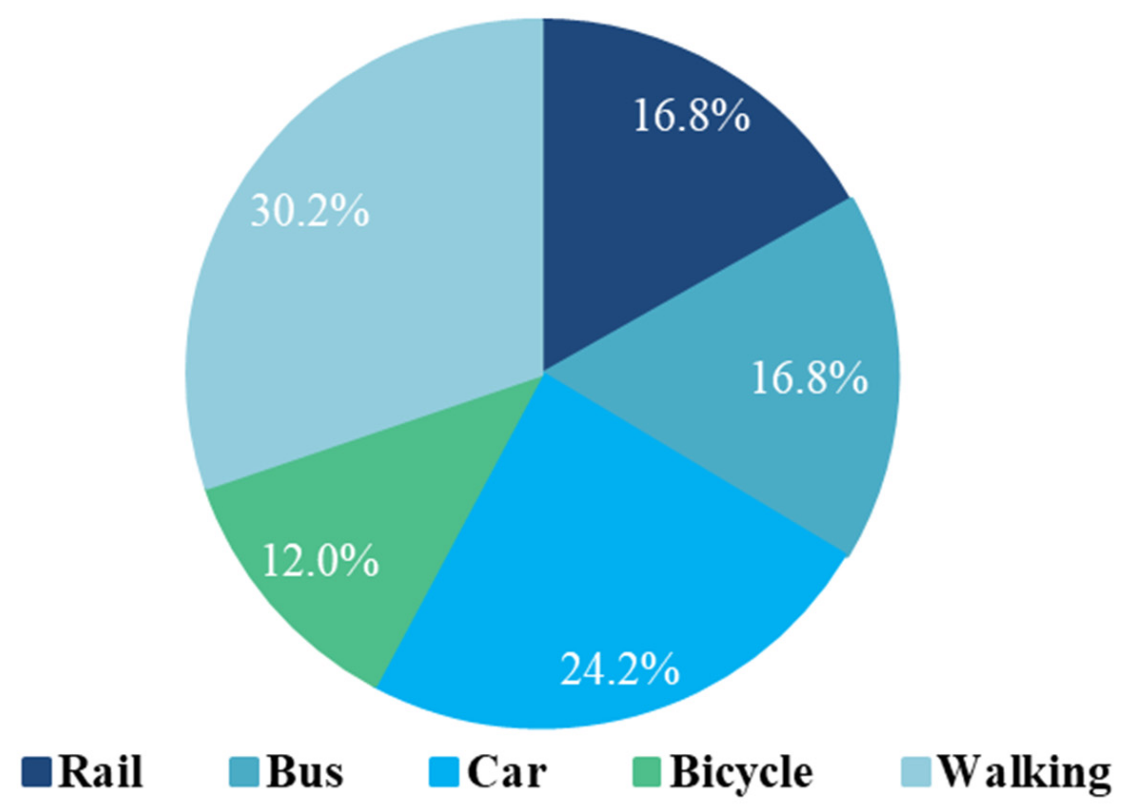
According to the “2019 BEIJING TRANSPORT ANNUAL REPORT” [22] (hereinafter refer to the “Transport Report”), the average daily travels in the central city area in 2018 were 39.24 million (including walking), among which the average daily travels of walking was the largest, reaching 11.45 million, followed by the average daily travels of cars, reaching 9.16 million, followed by rail transit, regular bus, and bicycle. In order to simplify the problem, this article will not consider taxis and other modes of travel that account for a relatively small proportion and determine the probabilities of various modes of travel based on the proportion of the remaining five modes of travel. The probability of various modes of travel is shown in Figure 2.

Considering that the electricity consumption levels of households with different economic conditions are different, the choice of mode of transportations is not the same, which will have a greater impact on the final simulation results. Therefore, in order to reflect this difference, households are typified according to their electricity consumption levels. The five groups I, II, III, IV, and V represent the office worker families with low, medium, and high levels of electricity consumption, elderly families, and mixed families (office worker + elderly), respectively. The probability distribution of travel mode selection of various families is shown in

Table 1. Probability distribution table of various modes of transportations (%).

Mode of Transportation a	Type I	Type II	Type III	Type IV	Type V
Rail	19.0	16.8	12.4	-	19.0
Bus	19.0	16.8	12.4	-	19.0
Car	14.2	24.2	44.2	-	14.2
Bicycle	13.6	12.0	8.8	-	13.6
Walking	34.2	30.2	22.2	-	34.2

. Among them, type II families take the city’s average level, type I and V families reduce the probability of car travels by 10%, type III families increase the probability of car travels by 20%, and the probability of other modes of transportation was distributed in the same proportion with each other in the “Transport Report” [22]. Type IV families generally travel less, mainly on foot, and the time consumption is usually short. Therefore, this paper does not consider their travel behavior, but only considers other activities at home including dinner, entertainment, etc.

Travel Time b

According to the relevant data in the “Transport Report” [22], the travel time of various modes of transportations in the morning peak in Beijing urban areas obeys normal distribution. It is assumed that the probability of the first travel time of residents with various travel modes on weekdays follows a normal distribution. The probability density function is:

$$\mathrm{f}\left(b\right)=\frac{1}{{\mathsf{\sigma }}_0\sqrt{2\mathsf{\pi }}}\exp [-\frac{{\left(b-{\mathsf{\mu }}_0\right)}^2}{2{\mathsf{\sigma }}_0{}^2}]$$

(1)

where b is the travel time; μ₀ and σ₀ are the mean and standard deviation of the normal distribution, determined by mode of transportation a.

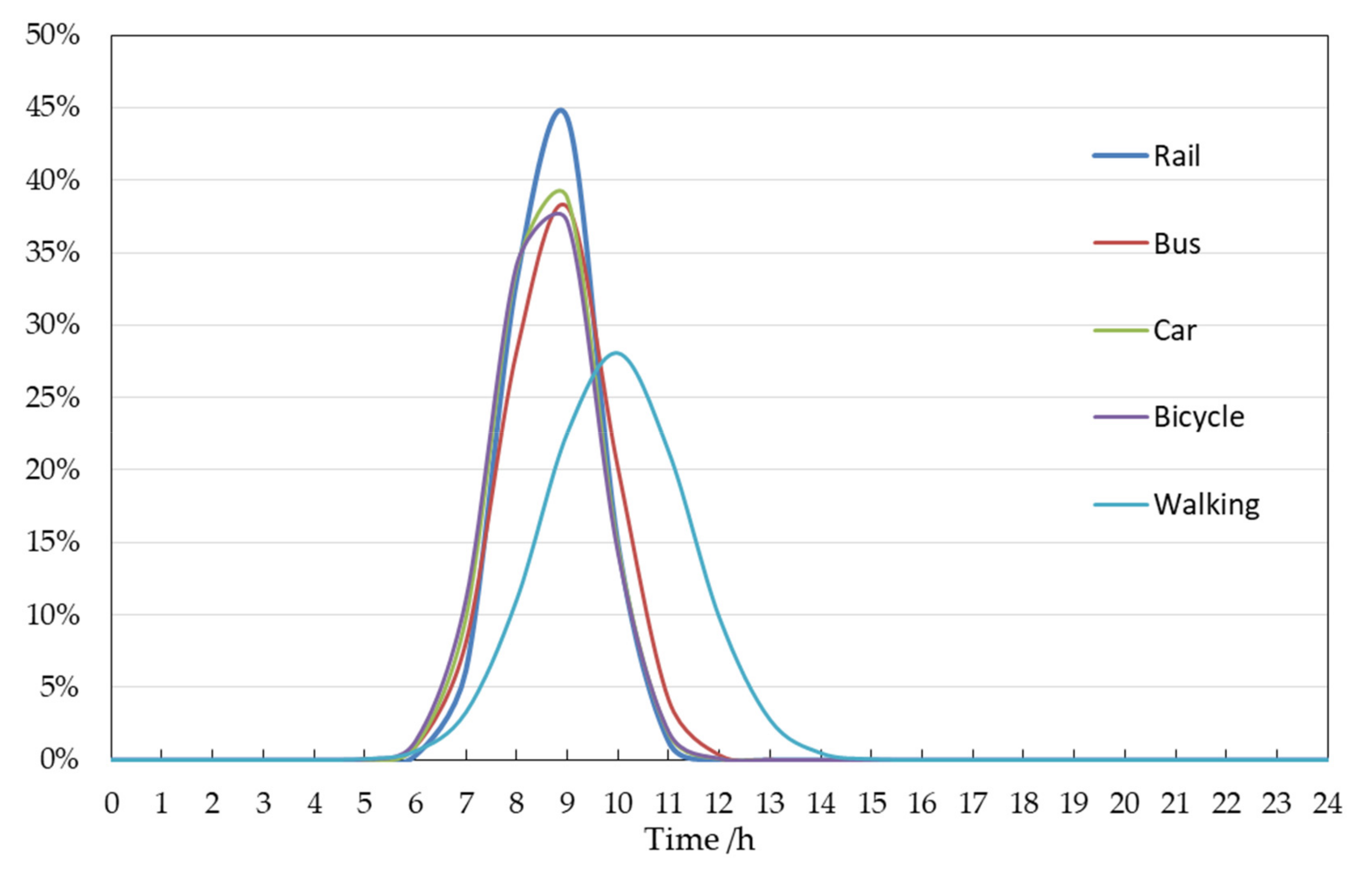
In this paper, a day is divided into 1440 minimum time units by taking 0 a.m. every day as the starting point and 1 min as the minimum measurement unit of time. By fitting the probability density function of the travel time of each travel mode in the “Transport Report”, the values of each parameter are obtained as shown in

Table 2. Parameters of the first travel time of various modes of transportation.

Mode of Transportation a	μ0 (hour)	σ0 (hour)
Rail	7.71	0.85
Bus	7.82	1.03
Car	7.62	0.95
Bicycle	7.58	0.98
Walking	8.94	1.42

, and the probability density curve of each travel mode is shown in Figure 3.

Time Consumption of Travel c

According to the research conducted by Beijing Transport Institute [23], with the IC card-swiping data of 31 days in August 2018 as the sample, travel time consumption of various travel modes approximately satisfies lognormal distribution. Its probability density function is:

$$\mathrm{f}\left(c\right)=\frac{1}{{\mathrm{t}\mathsf{\sigma }}_{\mathrm{t}}\sqrt{2\mathsf{\pi }}}\exp [-\frac{{\left(\ln c-{\mathsf{\mu }}_{\mathrm{t}}\right)}^2}{2{\mathsf{\sigma }}_{\mathrm{t}}{}^2}]$$

(2)

where c is the time consumption of travel; μ_t and σ_t are the mean and standard deviation of the lognormal distribution, determined by mode of transportation a.

Parameters of the probability density function of travel time consumption of various travel modes are shown in

Table 3. Parameters of probability density function of travel time consumption by various modes of transportation.

Mode of Transportation a	μt (min)	σt (min)
Rail	37.4	11.2
Bus	33.2	8.0
Car	23.6	5.7
Bicycle	22.3	1.8
Walking	11.4	1.1

, and the probability density curves are shown in Figure 4.

Travel Destination d

According to different travel destinations, each functional area can be divided into five types: Residential area H, work area W, shopping and entertainment area SE, social relaxing area SR, and other functional areas O. Residential areas refer to residential communities. Working areas mainly include large commercial office buildings, industrial parks, scientific research parks, etc. Shopping and entertainment areas mainly include large shopping malls, supermarkets, hotels, etc. Social relaxing areas mainly include parks, sports fields, scenic spots, and restaurants, etc. Other functional areas mainly refer to areas other than the aforementioned areas, such as government institutions, schools, hospitals, etc.

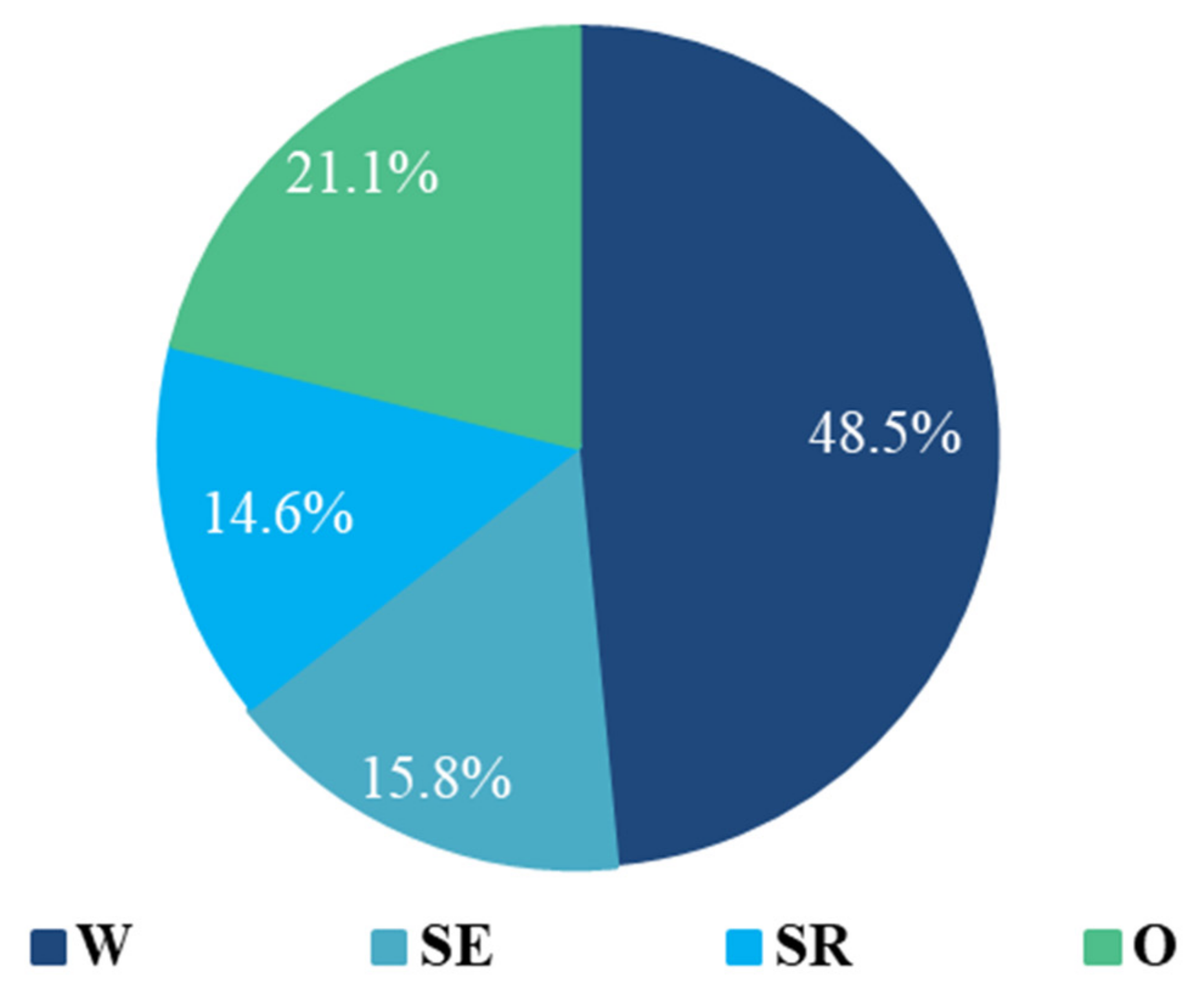
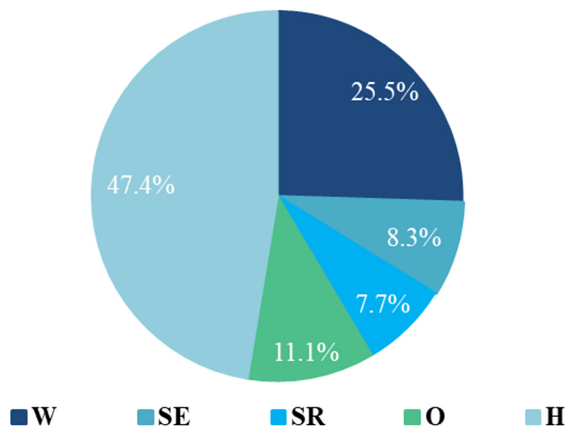
Generally speaking, the travel destination during the morning peak on weekdays is usually W or O, while the travel destination during the rest of the time is mainly H, SE, or SR. According to the “Transport Report”, in 2018, commuting travels accounted for 51% of the total travels, travels for shopping accounted for 8.3%, travels for entertainment accounted for 7.7%, travels for going home accounted for 21.9%, and other travels accounted for 11.1%. In this paper, the residential area is taken as the starting point to construct the corresponding travel chain. Since the destination of the first travel cannot be home, the probability of first travel to each destination was distributed in the same proportion with each other. The travel probability to the destination of the first and non-first travels are shown in Figure 5 and Figure 6.

Destination Stay Time e

The residence time of residents in each destination will significantly affect the formation of the travel chain, but there are few studies related to the residence time of residents in various urban functional areas at present. According to the study by Zhao et al., the probability density of the residence time in each functional areas follows the generalized extreme value distribution [24], wherein:

$$f\left(e\right)=\frac{1}{\sigma }\exp \left[{\left(1+\xi \frac{e-\mu }{\sigma }\right)}^{-\frac{1}{\xi }}\right]\times {(1+\xi \frac{e-\mu }{\sigma })}^{-\frac{1}{\xi }-1}$$

(3)

where e is destination stay time, and ξ, σ, and μ are three parameters of the generalized extreme value distribution. The value of parameters in W area is: σ = 164.506, ξ = −0.234, μ = 438.445. The value of parameters in SE, SR, and O areas is: σ = 41.761, ξ = 0.657, μ = 68.520.

The probability density curves of destination stay time are shown in Figure 7.

2.2.2. Household Power Load Level

On the basis of the travel chain model of residents, this section firstly determined the power load level under the combination of various common home appliances based on the power of each appliance, which is the basis for the final determination of the power load level of various households in different time periods. Then the electricity consumption period of a day is divided to build the household power load static level of five types of families under different scenes, which is the basis of the Monte Carlo simulation.

Combined Power of Common Household Appliances

The load level of common household appliances is shown in

Table 4. List of common household appliances power [25].

Household Appliances	Rated (Running) Watts	Additional Surge Watts
Essential Appliances
Electric Water Heater	4000 W	0 W
Light Bulb (LED)	9 W	0 W
Tube Light (1500 mm)	22 W	0 W
Window AC (10,000 BTU)	1200 W	3600 W
Air Purifier	25 W	5 W
Fan (Pedestal)	50 W	10 W
Kitchen Appliances
Cooker Hood	20 W	10 W
Dishwasher	1500 W	1500 W
Electric Kettle	1200 W	3000 W
Electric Oven	2150 W	0 W
Microwave	1000 W	0 W
Modern Fridge (2001–2020)	400 W	600 W
Rice Cooker	200 W	500 W
Laundry Appliances
Hair Dryer	1250 W	0 W
Vacuum Cleaner	200 W	200 W
Washing Machine	1150 W	2250 W
Entertainment Appliances
Computer Monitor	25 W	5 W
Desktop Computer	100 W	350 W
Home Internet Router	5 W	15 W
Set Top Box	27 W	3 W
Television (49” LED)	85 W	0 W
Television (82” LED)	230 W	65 W

.

According to Table 4, the average power of the combination of common household appliances in each specific period of time is shown in

Table 5. Average power of the combination of common household appliances.

Appliance Combinations	Time Period	Average Power (W)
Basic consumption (refrigerator, etc.)	All day	200–300
Kitchen appliances (breakfast and lunch)	Get up-go out	1200–1500
Kitchen appliances (supper)	Get Home-supper	1500–2000
Water Heater (standby)	All day	150–200
Water Heater (used)	Supper-sleep	500–600
Entertainment (day)	an hour after getting up- dinner	100–150
Entertainment (night)	Supper–sleep	300–500
Air conditioning		1000–1200
Electric fan		50

.

Division of Power Usage Period

Since there are many factors affecting residents’ electricity consumption behavior, in order to simplify the problem and facilitate the simulation, a day is first divided into six periods according to the correlation between residents’ outdoor behavior and electricity consumption. The division of each period is shown in

Table 6. Time division table of the residents’ travel model.

Time Period	Resident Behavior	Time Range
A	Sleep	22:00- wake up the next day
B	breakfast	Within 1 h after getting up
C	Going out/Staying home for the elderly	After breakfast–go home (office worker)
		After breakfast–dinner (elderly)
D	Elderly lunch	12:00 around
E	Supper	Within 1 h after returning home (office workers)
		18:00 around (elderly)
F	Supper-sleep	After dinner- 22:00

.

Taking into account that the electricity consumption levels of different households are not the same, it will have a greater impact on the final simulation results. Therefore, in order to reflect the difference of electricity consumption levels among different types of households, the average power of common home appliance combinations in Table 4 is referred to in order to determine the load levels of different households in different periods, as shown in

Table 7. Power load tables for different periods of time in various types of households (Unit: Watt).

Time Period	Household Type
	I	II	III	IV	V
A	200	350	400	200	200
B	1400	1850	1900	1400	1400
C	200	350	400	300	300
D	200	350	400	1400	1400
E	1750	2850	3400	1250	1750
F	1050	2000	2300	550	1050
E (no cooling load)	1700	1850	2400	1200	1700
F (no cooling load)	1000	1000	1300	600	1000

. In order to highlight the influence of cooling load on the distribution of residential power load, loads in periods E and F are divided into two situations: With cooling load and no cooling load, which respectively represent the power load in hot weather and cool weather in summer in Beijing.

Period A and C: Type I households pay more attention to saving electricity. For example, they will consciously turn off the water heater when no one is taking a bath to reduce electricity consumption, etc. Therefore, the “basic consumption” is taken as the electricity consumption level of type I households during period A and C. Households of type II and III have additional average standby power of the water heater during these two periods (150 W and 200 W, respectively). Since the elderly of Type IV and V families seldom go out and mainly watch TV for entertainment, the power load in period C is higher (100 W) than that of Type I families.

Period B: On the basis of the load in period A and C, the average power of cooking breakfast (1200 W for type I, IV, V households, 1500 W for type II and III households) is added as the power load in period B.

Period D: That is, the power load during lunch period. For type IV and V families, it consists of “basic consumption” and the average power of cooking lunch using kitchen appliances (1200 W). For type I, II, and III households, the load is exactly the same as period C.

Period E: Due to the hot weather in summer in Beijing, it is assumed that the fan (50 W) will be turned on in Type I, IV, and V families from the time they get home until going to bed, while the air conditioning (1000 W) will be turned on in Type II and III families during the same time. Considering that the forms of cooking and entertainment are relatively single in Type IV households, “basic consumption” and the average power of using kitchen appliances to cook dinner (1000 W for Type IV households, 1500 W for Type I, II, V households, 2000 W for Type III households) will be added as the power load in Period E.

Period F: From dinner to bedtime, residents usually take showers and participate in recreational activities. Considering that the demand for bathing and entertainment is low in Type IV households, their electricity consumption level in period F is lower than that of Type I families. On the basis of “basic consumption”, the average heating power of a water heater (250 W for Type IV households, 500 W for Type I, II, V households, 600 W for Type III households) and electricity consumption of electric fans (50 W), air conditioning (1000 W), and entertainment equipment (150 W for Type IV households, 300 W for Type I, II, V households, 500 W for Type III households) are added as the HPL in period E.

2.2.3. Simulation Process Based on Monte Carlo Method

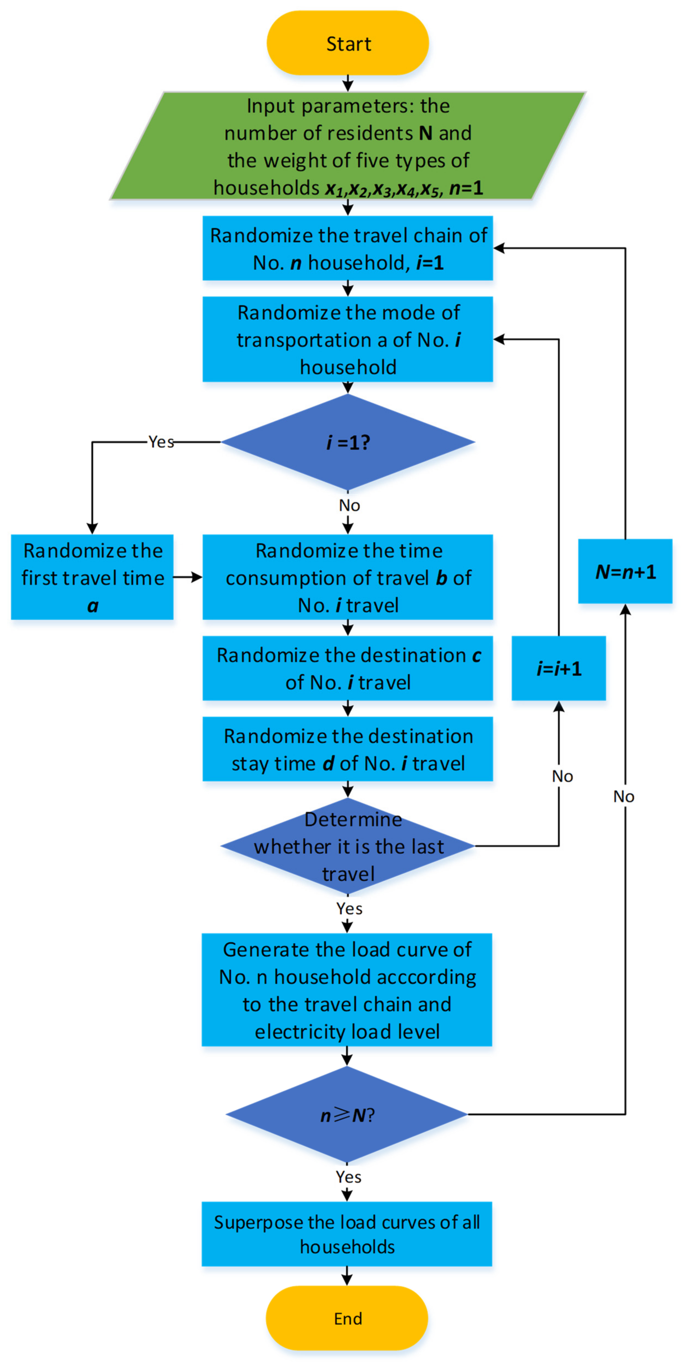
In this paper, the total number of residents in the region is set as N, and the proportion of residents of Type I, II, III, IV, and V is set as x₁, x₂, x₃, x₄, and x₅, respectively. Each resident shall travel at least 2 times per day and no more than 6 times, and the total time spent on travels in a single day shall not exceed 10 h. Each travel shall be counted as one time for each destination. The Monte Carlo method is used to simulate the electricity demand of each residential user, and then the time distribution of residential power load demand based on travel chain is solved.

The simulation takes the time t₀ as the starting point. First, according to the probability density function, the mode of transportation, travel time, time consumption of travel, and travel destination are sequentially generated. Secondly, the destination stay time and the next travel are generated according to the probability density function. Then, according to the total number of travels, the cumulative time of travels and the next destination, as well as whether the next travel is the last one, is judged. If the next travel is the last one, the time distribution data of the power load demand of households will be generated; if not, the program will determine the next travel destination and continue to calculate the travel chain until the last one. Finally, the time distribution data of all residential users are counted to form the distribution curves of residential power load demand of five types of households. The whole solution process is shown in Figure 8.

3. Results

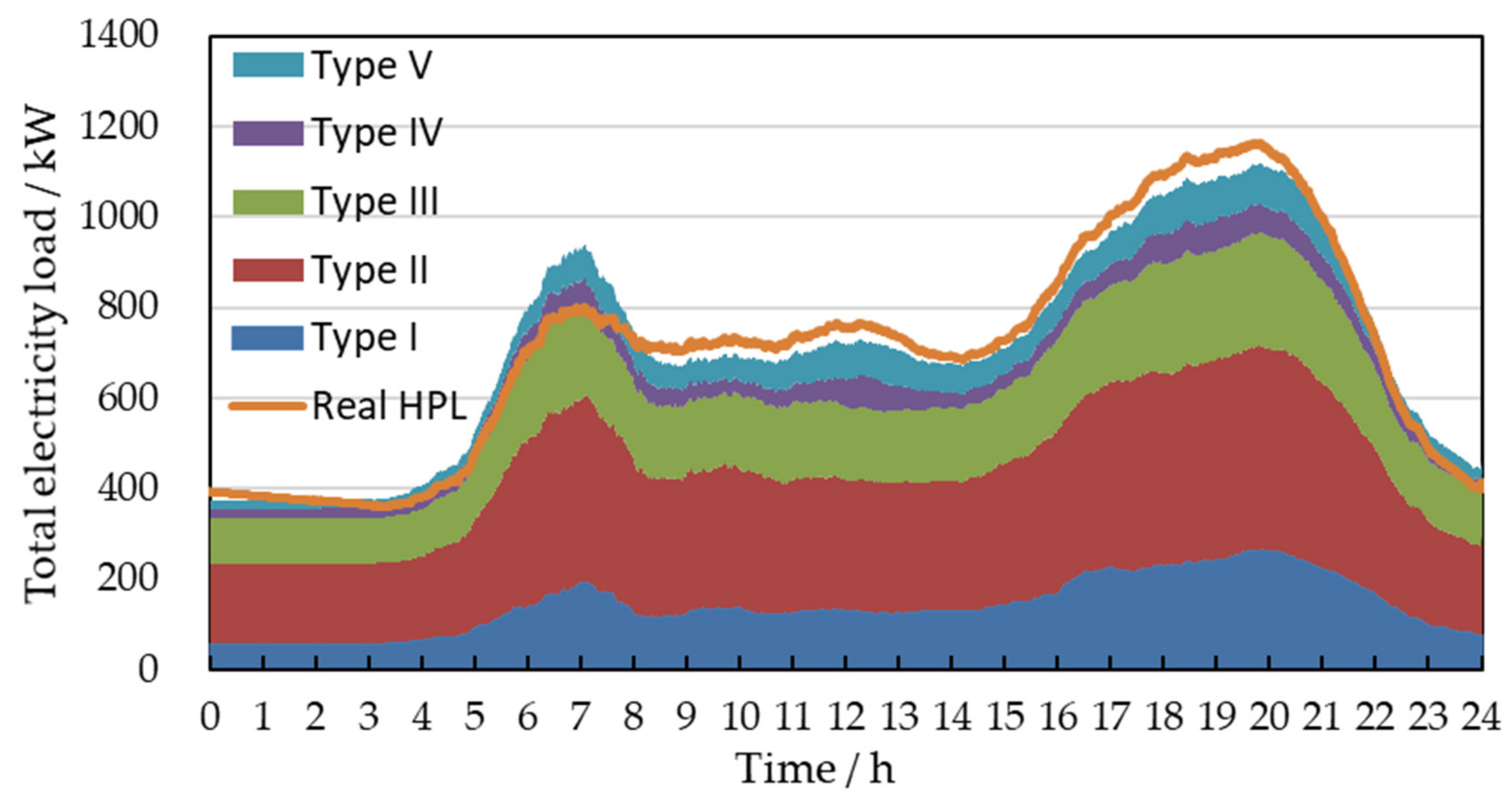
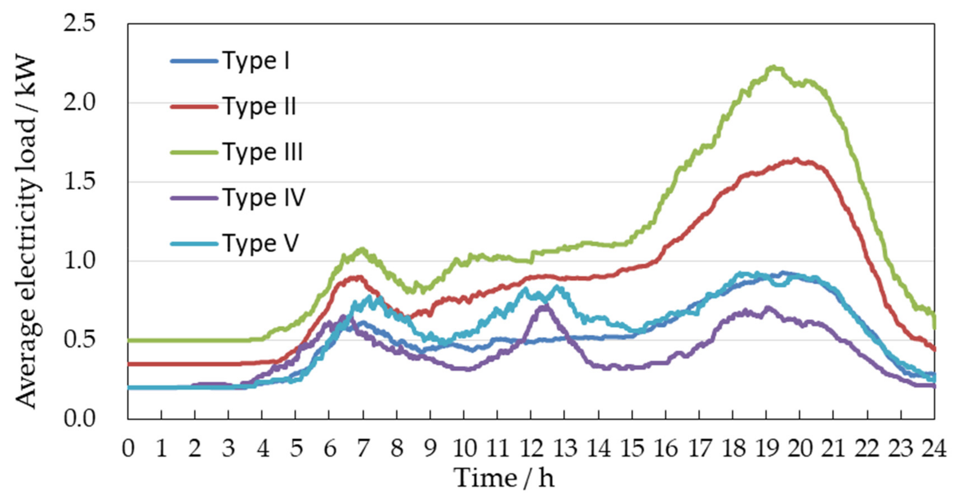
The total number of households set in this simulation was 1200, with the Type I family accounting for 25.0%, Type II family accounting for 41.7%, Type III family accounting for 16.7%, Type IV family accounting for 8.3%, and Type V family accounting for 8.3%. A total of 3010 travels were obtained after the simulation, in which the destination W accounted for 30.33%, the destination O accounted for 13.62%, the destination SE and SR accounted for 9.60% and 9.90% respectively, and the destination H accounted for 36.54%. 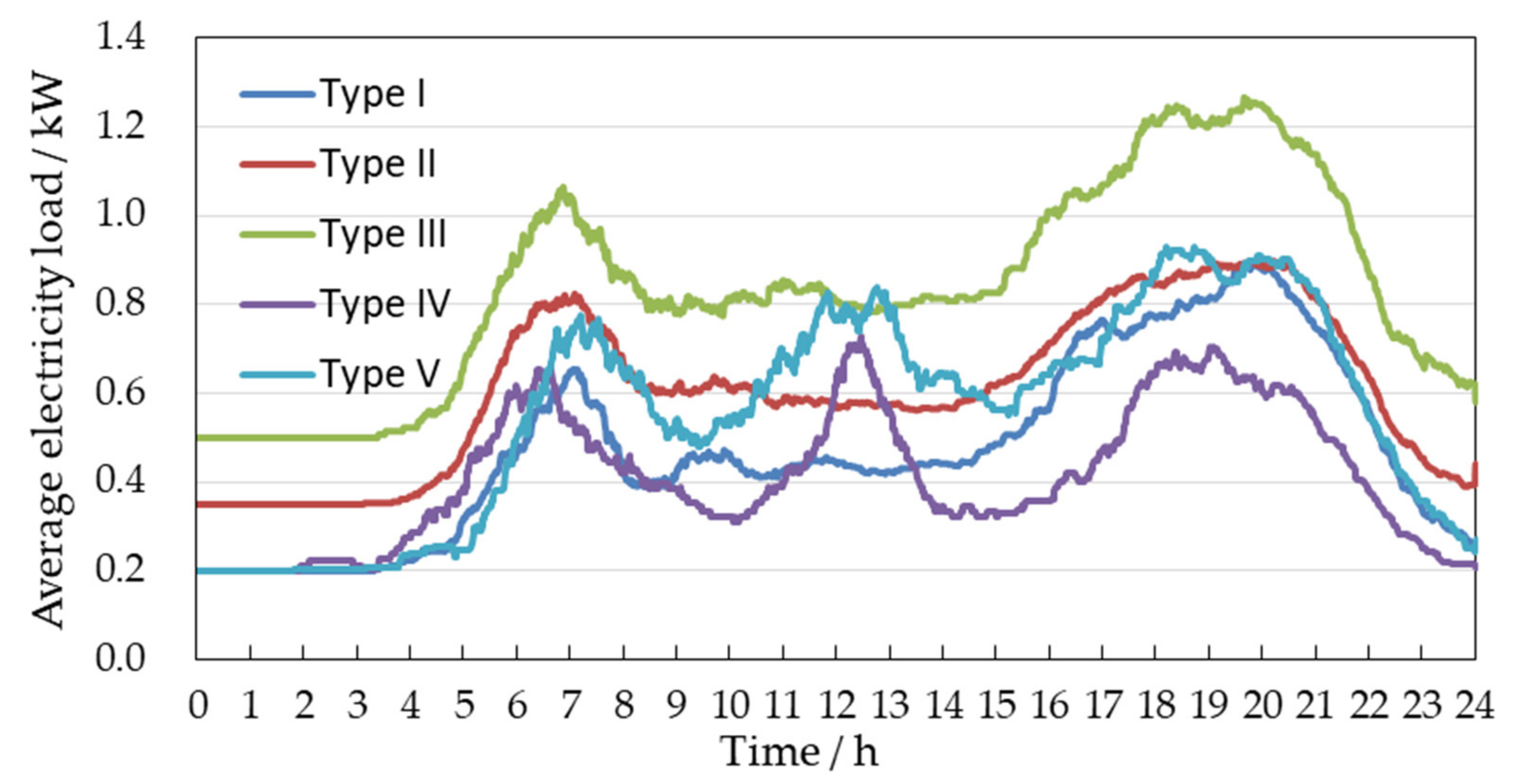The total power load curves of five types of households (with cooling load/no cooling load) are shown in Figure 9 and Figure 10, where the typical summer load curves of a community in Beijing was introduced to verify the feasibility of the model. The average power load curves (with cooling load/no cooling load) of five types of households are shown in Figure 11 and Figure 12.

3.1. Total Electricity Load Level

Above all, by comparing the simulation results (stacking area chart) and typical load of community (line chart) in Figure 9 and Figure 10, it can be seen that the variation trend of them is basically the same, and the maximum deviation is only about 10%, which indicates the validation of the simulation model. The peak at noon shows great difference between simulation and the real situation. The most likely reason is an overestimation of load levels around the morning peak.

An analysis of Figure 9 reveals that in terms of the total load, the HPL of Type II families takes the main part, which is closely related to its relatively high proportion (41.7%). The proportion of Type III households (16.7%) is lower than that of Type I households (25%), but due to their higher power consumption levels, the load level of Type III households is higher throughout the day than that of Type I households. The relatively low proportion (8.3%) and load level of Type IV and V households mean they have little influence on the trend and peak of the total load curve.

From the perspective of peak load, there are three obvious peak electricity consumption periods throughout the day, which are around 7:00, 12:30, and 19:30, respectively. The maximum load in the evening reached nearly twice the peak power consumption than the morning.

The analysis of Figure 10 shows that in cool weather, the contribution of all types of households to the total power load before 12:00 is similar to that in hot weather (Figure 9), but from 12:00 to the evening, the contribution of Type II and III households to the total power load decreased while the contribution of type I, IV, and V households increased. Moreover, the gap between the morning and evening peak is greatly reduced, which is mainly affected by the significant reduction of cooling load of Type II and III households.

3.2. Average Electricity Load Level

An analysis of Figure 11 reveals that in terms of the total load, the electricity consumption level of the five types of households presents the following trends: III > II > V> I > IV. This is consistent with the basic characteristics of five types of families.

From the perspective of peak load, there are two peak periods of HPL for Type I, II, and III households throughout the day, at 6:00 and 20:00, respectively. Type IV and V households have three peak hours of electricity consumption throughout the day, which are around 6:30, 12:00, and 20:00, respectively. The new peak of electricity consumption at noon is caused by the cooking for lunch by the elderly.

By comparing the average load curves of Type I, II, and III families separately, it can be found that the difference in the choice of travel modes of the three types of families has no obvious influence on the morning and evening peak hours of electricity consumption, which are all around 6:30 and 20:00. Since the random process and time period division of the travel chain of the three types of families are exactly the same, the differences are all caused by the choice of travel modes and the differences in the power load levels of each period. Therefore, the small difference may be caused by the fact that the probability difference of travel mode selection among the three families is not large enough, or the variance of the random process at the time of first travel is too large.

From the point of view of peak load, by comparing the load curves of Type II and III households to Type I, IV, and V households, it can be found that the power load in the evening peak period is higher than that in the mooning and the noon peak, due to the use of air conditioning in hot weather.

By comparing the average load curve of Type I, II, and III households alone, it can be found that the maximum load of the three types of households is around 20:00, among which the use of high-power electrical appliances such as air conditioning and water heater makes a great contribution to the peak value. This time is also the time when the maximum load of the Beijing power grid is concentrated in the hot weather in summer. Therefore, if no intervention is carried out, residential power consumption will cause great pressure on the safe and stable operation of the power grid.

By comparing the average load curve of Type I, IV, and V households alone, it can be found that the load curve of Type IV households shows a three-peak pattern with a significant peak and valley, and the difference between the peaks is not obvious, since the elderly are less likely to go out and there is a low demand for entertainment and cooling equipment. The morning peak load of Type V families is similar to that of the type IV family, but the afternoon peak and evening peak load are significantly higher, and the evening peak load is roughly the same as that of the Type I family. As the three types of households do not turn on the air conditioning during the day, the peak load of the evening peak is mainly affected by the entertainment and bathing load after the family members go out. Taking into account the load generated by entertainment equipment, which is difficult to control, water heater load is the electrical appliance with the greatest potential for control, excluding air conditioning. The peak load can be transferred without affecting normal use by reasonably setting the “time-temperature curve” of the water heater in a day.

An analysis of Figure 12 reveals that in terms of the peak load time, there is no significant difference between the peak time of morning and afternoon electricity consumption in cool weather and that in hot weather. However, the electricity consumption peak time in the evening for Type I, II, and III households is about 19:00, which is about one hour earlier than that in the hot weather. The main reason is that the decrease of cooling load causes the evening peak time to be more affected by cooking dinner, resulting in a forward deviation.

From the perspective of peak load value, it can be clearly seen from the comparison with Figure 11 that the evening peak load of Type II and III households using air conditioning in hot weather significantly decreases, while the evening peak load of Type I, IV, and V households without using air conditioning does not change significantly.

Separately comparing the average load curves of Type I, II, and III households, it can be found that the maximum load of the three types of households is around 19:00, and the peak load of type I and II households are close to the same. At this time, the use of water heaters and kitchen appliances contributes most to the peak value.

4. Discussions

The results obtained in this simulation are in line with the typical summer load curves of a community in Beijing, and the relative error is small enough to verify the feasibility of the model.

According to the average load curves of five types of families, it can be clearly seen that travel chains, temperature, and difference in electricity consumption level have great impacts on HPL. Considering that the difference in family characteristics will lead to different choices of travel modes, we set different probabilities of travel modes for Type I, II, and III households to reflect its influence on the load curves. Theoretically, the differences in travel mode selection of a large number of samples will affect the whole travel chain by affecting travel time and time consumption, which will ultimately affect power consumption behavior and peak load. However, in this simulation, the difference in the choice of mode of transportations for Type I, II, and III households does not have a significant impact on the morning and evening load peaks. The possible reason is that the probability difference of mode of transportation selection among the three types of families is not large enough, or the variance of the randomization of the first travel time is too large.

From the perspective of total power load, Type II households represent middle-income households, whose power load becomes the largest component of the total residential electricity load by virtue of its relatively high proportion and average electricity consumption level. They should be regarded as the key objects when considering residential electricity regulation.

Due to daytime work and the eating habits of Chinese people, cooking has become an important source of electricity load. In addition to natural gas, Chinese people often use high-power kitchen appliances such as microwave ovens, induction cookers, and rice cookers, which can cause a large, concentrated load. However, in general, the load generated by cooking is not easy for regulation.

Loads with the greatest regulatory potential are refrigerators and water heaters. From the above comparison, it can be seen that the evening peak load in cool weather is reduced by nearly half compared with that in hot weather, which is cooling loads. In fact, cooling loads account for about 40% of the maximum load in Beijing in summer, and the two tend to be the same. The water heater has high power during operation, but it also has the ability to store heat. We can save money on electricity bills and improve the load curve by presetting the water heater to operate during periods of low power.

For Type II and III households, the appliance with the most potential for regulation is the air conditioning, followed by the water heater, while the appliance with the most potential in Type I and V households is the water heater. Type IV families have low regulatory potential.

For type II and III households, incentive regulation strategy is advocated, such as reasonable control of air conditioning temperature, reduction of air conditioning in the HPL peak period, adjustment of preset heating time of water heater, etc., so as to transfer the peak load and improve the daily load curve of residents. For Type IV elderly families, due to the small potential in the regulation of electrical equipment and more feedback to the changes of electricity price, electricity price policy should be the main focus. For Type I and V households, price policy and incentive strategy can be used together due to their moderate regulation potential and sensitivity to electricity price.

5. Conclusions

Based on the travel chain of Beijing residents on working days, this paper considers the differences between travel chains, and studies the distribution of household power load of different types of households in summer. The load curves of the five types of households are compared and analyzed from the two aspects of total load and average load, explaining how the travel chains and the associated power consumption behaviors affect the residents’ power load. Electrical appliances with greater potential for regulation are determined and targeted regulation suggestions are put forward.

The results proved the feasibility and validity of the research method. On this basis, they reflect the influence of family characteristics and travel rules on HPL. Meanwhile, the household appliances with high regulation potential are found, which can provide reference for related policies to reduce the peak–valley gap and improve power efficiency. While the viewpoint is relatively novel, there are some cases of thoughtlessness or oversimplification in the method. For example, several elements of the residential travel chain are considered to be independent simulations, which are out of line with reality. Even so, we believe that the starting point of this paper is advisable. In the era of big data being gradually popularized, a detailed and comprehensive traffic statistical data may be used to predict residents’ load. If more detailed traffic statistics can be obtained later, combined with better models, many new conclusions may be obtained on the basis of this idea.