Abstract
In recent years, the integration of distributed generators (DGs) in radial distribution systems (RDS) has received considerable attention in power system research. The major purpose of DG integration is to decrease the power losses and improve the voltage profiles that directly lead to improving the overall efficiency of the power system. Therefore, this paper proposes a hybrid optimization technique based on analytical and metaheuristic algorithms for optimal DG allocation in RDS. In the proposed technique, the loss sensitivity factor (LSF) is utilized to reduce the search space of the DG locations, while the analytical technique is used to calculate initial DG sizes based on a mathematical formulation. Then, a metaheuristic sine cosine algorithm (SCA) is applied to identify the optimal DG allocation based on the LSF and analytical techniques instead of using random initialization. To prove the superiority and high performance of the proposed hybrid technique, two standard RDSs, IEEE 33-bus and 69-bus, are considered. Additionally, a comparison between the proposed techniques, standard SCA, and other existing optimization techniques is carried out. The main findings confirmed the enhancement in the convergence of the proposed technique compared with the standard SCA and the ability to allocate multiple DGs in RDS.
1. Introduction
Distributed generators (DGs) are energy devices that are attached directly to the distribution network or the consumption location. DGs introduce cleaner electricity production, as many DGs make use of renewable sources of energy such as wind and solar power. The integration of DGs has several merits such as reducing line losses, improving system reliability, decreasing fuel, power quality improvement, and raising efficiency.
Throughout recent years, the incorporation of DGs into the radial distribution system (RDS) has been growing rapidly in numerous regions of the world; the main causes for this growth are the liberation in energy markets, limits on constructing new transmission and distribution lines, and environmental riskiness [1,2,3]. Additionally, excessive technological progress in small generators, storage devices backup power, and power electronic devices have accelerated the permeation of DGs into power plants [4]. However, inappropriate placement of DGs may lead to undesirable results such as increasing power losses and energy costs. Hence, optimal allocation of the DGs is significantly required.
Numerous optimization algorithms have been used in the literature to identify the best location and size of the DG unit of both transmission and distribution networks [5,6]. In the power system, three optimization algorithms were implemented: the analytical algorithm, the heuristic algorithm, and a hybrid between the analytical and heuristic algorithms [7].
A mathematical formulation for the power system is thoroughly articulated in analytical algorithms to investigate the influence of the injected DG power on the performance of the power system, as provided in the improved analytical (IA), exhaustive load flow (ELF) optimization algorithms [8], iterative–analytical method [9], analytical method [10], and efficient analytical (EA) method [11]. Additionally, several indices were determined with differential equations [12] such as LSFs, which have been introduced to specify the candidate buses for DSTATCOM allocation [13]. However, some of the analytical algorithms are not suitable to find the optimal size and location of multiple DGs [14].
As a result, several researchers switched to metaheuristic-based optimization algorithms. The key feature of using metaheuristic algorithms is their ability to solve optimization problems without going too deep into the complexity of the problem. Metaheuristic optimization algorithms have also been commonly used in DG allocation. The most popular meta-heuristic techniques that have been used to allocate the DG in RDS are the backtracking search optimization algorithm (BSOA) [15], ant lion optimizer (ALO) [16], grey wolf optimizer (GWO) [17], whale optimization algorithm (WOA) [18], moth-flame optimizer (MFO) [19], bat optimization algorithm (BA) [20], Krill herd algorithm (KHA) [21], and salp swarm algorithm (SSA) [22]. However, the metaheuristic algorithms face some issues such as trapping in the local optima and low convergence rate.
Hence, hybrid techniques have been developed to avoid the issues of the analytical and metaheuristic algorithms such as multi-objective hybrid teaching–learning-based optimization–grey wolf optimizer (MOHTLBOGWO) [23], a hybrid configuration of the weight improved particle swarm optimization (WIPSO) algorithm and gravitational search algorithm (GSA) called the hybrid WIPSO–GSA algorithm [24], hybrid fuzzy-particle swarm optimization (PSO) [25], and hybrid analytical-PSO [26].
In this paper, a hybrid between analytical and metaheuristic optimization algorithms is developed to optimally allocate multiple DG units into RDS. The main advantage of this hybridization is to gain advantages and avoid the drawbacks of these two techniques. Hence, the main contributions of this work are summarized as follows:
- Proposing candidate bus selection using loss sensitivity factor (LSF) with the fuzzy logic controller.
- Proposing a hybrid between the analytical technique and sine cosine algorithm (SCA).
- Applying the proposed hybrid technique to determine the optimal allocation of DG units in RDS to minimize the total losses.
- Checking the performance of the proposed hybrid technique compared to the conventional SCA and other well-known optimization methods using standard IEEE 33-bus and 69-bus RDS.
In the present work, three types of DGs are used as follows:
- Type I: Injects only active power.
- Type II: Injects only reactive power.
- Type III: Inject active and reactive power.
The remainder of the paper is organized as follows: Problem formulation including power flow equations and objective functions is summarized in Section 2. Section 3 illustrates the proposed methods including the hybrid technique and SCA. Section 4 illustrates the proposed hybrid optimization technique. Section 5 discusses the simulation results. Finally, the main results are outlined in Section 5.
2. Problem Formulation
The main target of the proposed hybrid method is to find the best locations and capacities of the DGs that minimize the total power losses subjected to multi constraints in the radial distribution networks.
2.1. Power Flow Equations
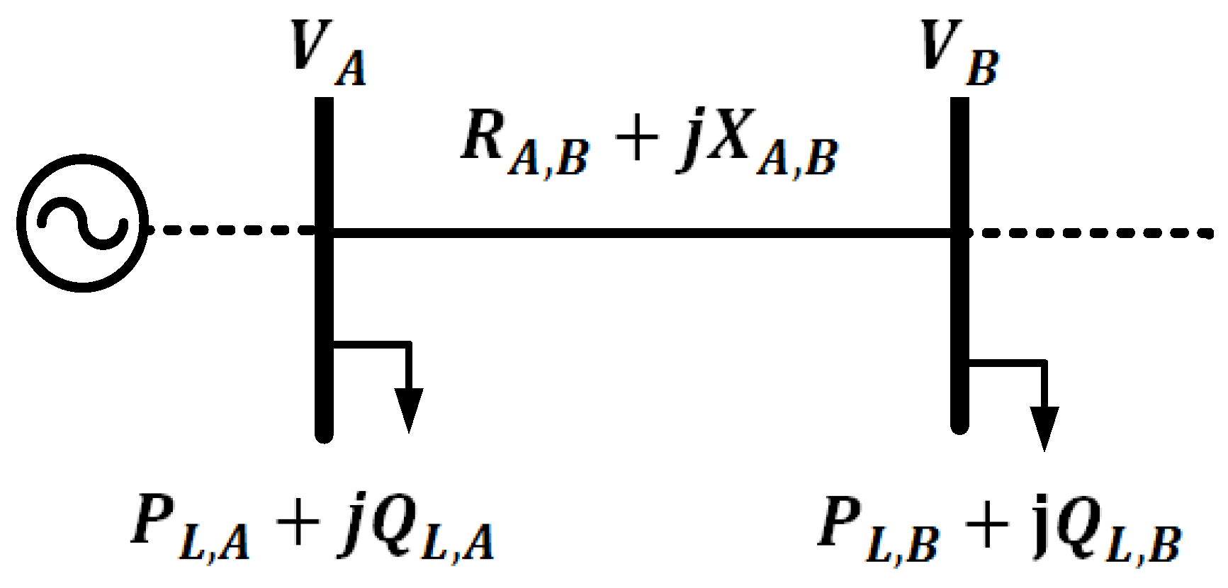
To determine load flow in the distribution system, Figure 1 is a portion of the single line diagram of RDS; A is sending bus and B is receiving bus. Then, active and reactive powers can be calculated using Equations (1) and (2).
where are the active powers at buses respectively, and are the reactive powers at buses respectively. represent the active and reactive load power at bus B, respectively. and express the resistance and reactance of lines A, B, respectively. is the voltage at bus B and can be calculated with the voltage at bus A () using (3):
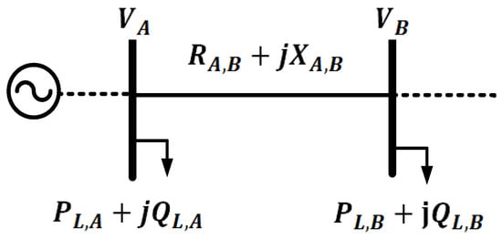
Figure 1.
A simple two buses of RDS.
Therefore, active power loss in the line between buses A and B can be calculated as:
and the reactive power loss in the line between buses A and B can be calculated as:
Hence, total active and reactive power losses) in RDS can be calculated by the summation of the losses for all branches in the power system:
2.2. Objective Function
In general, installing the DGs units in RDS lead to current flow reduction in the feeders, which in turn decreases power losses and enhances voltage profile. In the present work, minimizing active power losses is the main objective function, which can be formulated as:
where and can be calculated as follows:
2.3. Problem Constraints
The DG allocation must be subject to the following constraints.
2.3.1. Power Balance Equation
In order to prevent reversing power, a balance between generation and demand for power plus power loss should be considered, and thus this restriction can be expressed as:
where and are the active and reactive powers of the main substation, respectively, and are the active and reactive powers of the DG at bus, and and are the load active and reactive powers., , and are the total number of DGs, buses, and branches respectively.
2.3.2. Inequality Constraints
The operating limits of the distribution systems must be assessed, for example:
DGs capacity limits:
Voltage Limits:
The voltage at each bus must be within the limits.
3. Overview of the Optimization Methods
In the present work, a hybrid technique based on candidate bus selection, analytical technique, and SCA is introduced to solve the placement of three types of DGs for multiple DGs. LSF is used to identify the candidate buses for the DGs locations, while the analytical technique is implemented to determine the best sizes of the DGs at the combinations of the candidate buses; then, these values are used as the initial values in SCA to specify the optimal locations and sizes of the DGs.
3.1. Candidate Buses Selection
LSF is introduced to identify the locations of the DGs in the RDS by determining the buses that are more sensitive to the injected active and reactive powers. Using the normalized LSF and voltage magnitude on each bus, a fuzzy logic controller is applied to arrange the system buses according to the fuzzy weighting output. The candidate buses for the DG placement are selected based on the highest output weighting buses. These candidate buses can reduce the search space of the optimization algorithm.
Let consider two buses m-1, m connecting with impedance that have active and reactive power loads . If at a bus delivers the active power beyond that bus, the LSF can be assumed by:
Two inputs and one output are used for a fuzzy controller. NLSF is the first input and can be expressed as follows:
where all are between [0, 1].
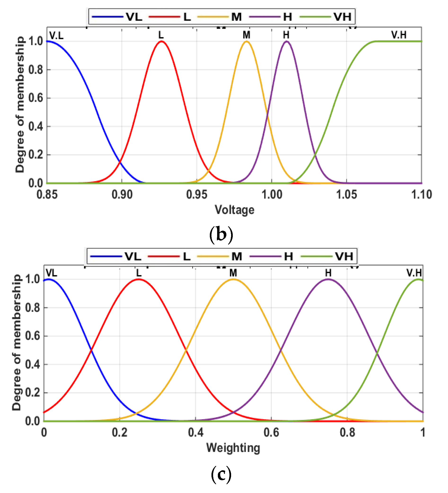
The fuzzy output can be obtained through three stages: fuzzification, IF-then rules, and defuzzification. The input and output are replaced by a different membership function (MF) based on its value. To represent the , five membership functions are included as seen in Figure 2a. The memberships are named as very low (VL), low (L), medium (M), high (H), and very high (VH), where a Gaussian form is used to model these memberships. The second input is the voltage profile on each bus and, as seen in Figure 2b, is defined by five membership functions. The fuzzy output is estimated based on (IF, Then) predetermined 25 rules, as given in Table 1. Hence, each bus will get a weighting value based on its voltage and. For instance, if a bus has a voltage equal to 0.93 p.u, which is represented by L (see Figure 2b), and equals 0.5, which is M (see Figure 2a), then the output will be calculated using Table 1, and it gives M, as presented in Table 1. Finally, the weight output value can be calculated using Figure 2c, which equals 0.51. The above procedure will be applied for all buses, and the values are classified as a candidate bus in descending order.
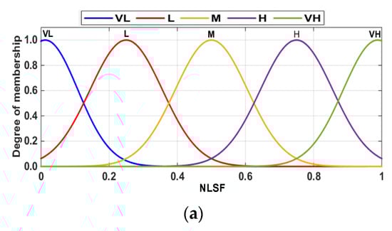
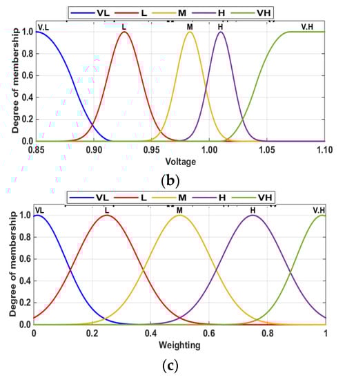
Figure 2.
Fuzzy inputs and output memberships. (a) Membership function for NLSF (b) Membership function for voltage magnitude (c) Membership function for weighting.

Table 1.
Fuzzy rules.
3.2. Analytical Technique
From Figure 1, the power loss () in the RDS can be determined by the exact loss formula equation as (1).
Let us consider as the number of the DGs of Type I, and their locations are , while are the sizes of the DGs, respectively.
Therefore, the active power supplied from Type I can be:
Additionally; is the number of the DGs of Type II, and their locations are , while are the capacities of the DGs, respectively.
The reactive power supplied from Type II can be:
The best objective function can be obtained if the first derivative of losses respects the power delivered from the DG become zero; so, it can be assigned as:
or
and the differential of the active power loss according to active power injection can be written as:
or
Additionally, the differential of the power loss with respect to reactive power injection can be written as:
Similarly, the differential for:
After rearranged the previous equations, they can be formulated as illustrated below:
where
Let us suppose matrix (27) equal to the following equation (30).
Then after being rearranged, it becomes:
Next,
Then,
Finally, the optimal size of Type I of the DG installed at the bus can be calculated from the following equation:
: Active power load at bus.
Additionally, the optimal size of Type II of the DG installed at bus can be determined from the following equation:
: Reactive power load at bus
Note that:
- In the case of installing Type I of the DG ;
- In the case of installing Type, I Type II of the DG ;
- In the case of installing Type, I Type III of the DG .
The power factor () of Type III can be determined using (36) and (37), in the case of , which can be formulated as:
In the case of a single DG allocation, it would be easy to use these calculations because the number of the combinations is the total bus number. However, for multiple DG allocation, the number of combinations is NCr where N is the number total of buses and r is the number of the DGs, and that would be a more exhausted calculation. Hence, a hybrid between analytical and meta-heuristic is a good solution for multiple DG allocation.
3.3. Sine Cosine Algorithm (SCA)
SCA is a metaheuristic optimization algorithm proposed by Mirjalili [27]. The main idea behind this algorithm is to use the sine and cosine functions to find the optimal global solution. Several individual solutions are randomly distributed in the SCA and then the fitness function is determined for each solution. The following steps are used to implement the SCA.
Steps of SCA:
- Step 1
- Specify the parameters of the sine cosine algorithm such as search agent number, number of the maximum iterations.
- Step 2
- Initialize the population of solutions randomly within the upper and lower borders of variables as follows:where i is the search agent number and j is the variables number (dimension).
- Step 3
- The situation for the population of solutions can be assigned as follows:
- Step 4
- Determine the objective function amount according to the search agent situation as follows:
- Step 5
- Calculate the purpose of fitness that is known as a preferable fitness and the purpose position that is known as a preferable position.
- Step 6
- Update the situation of the search agent as presented as follows:where is a variable that used to balance between the exploration and exploitation phases and can be expressed as follows:are random variables and expressed as follows:
- T is the current iteration.
- is the maximum iteration.
- is the objective global best solution.
- Step 7
- Iterate the steps from 3 to 5 until the standing criteria are ascertained.
- Step 8
- Acquire the optimal destination fitness and the optimal destination.
3.4. Proposed Hybrid Optimization Technique
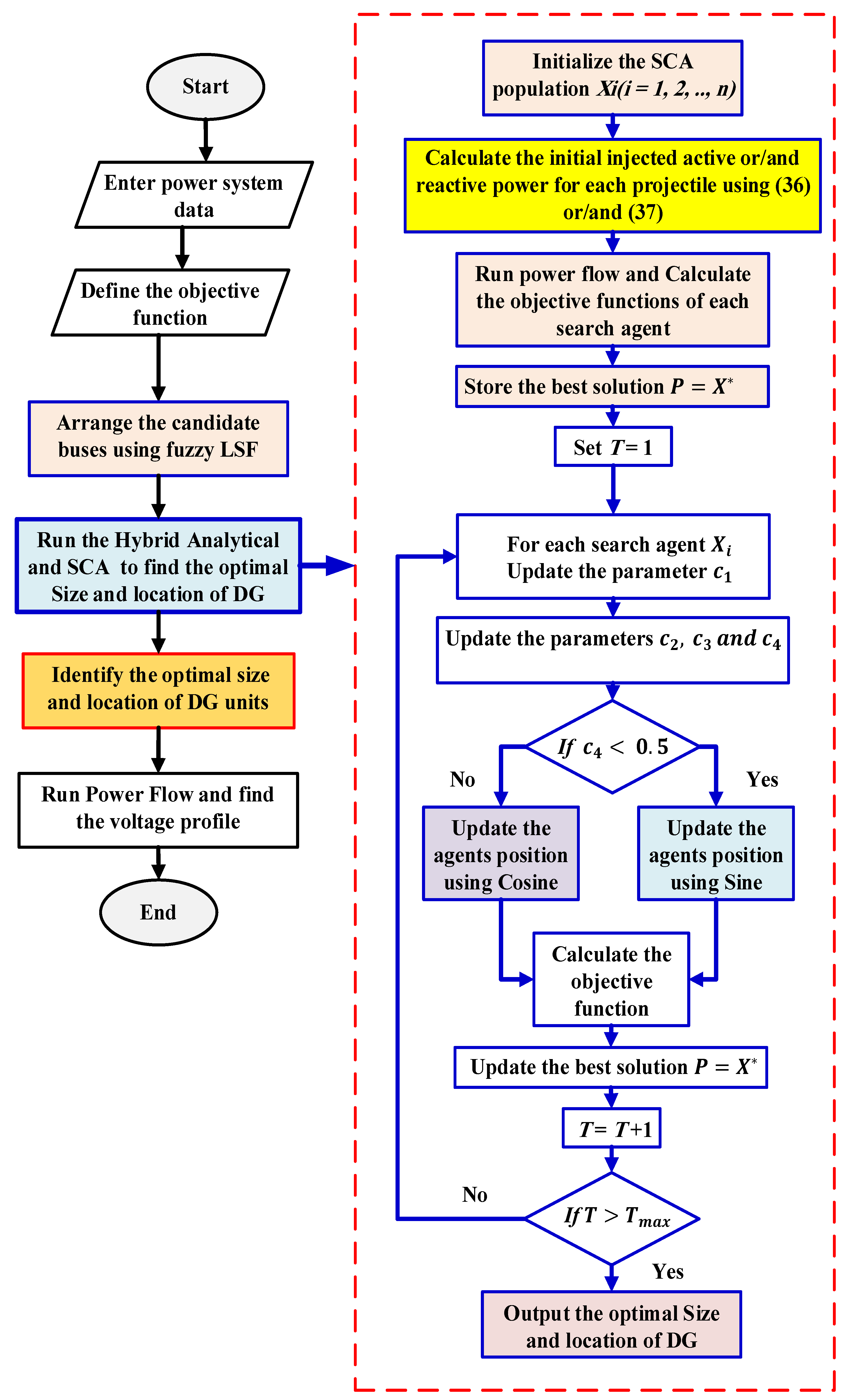
The computational procedure of the proposed hybrid analytical–SCA technique to find the proper sizes and locations of the DGs in order to obtain minimum losses. Figure 3 presents the flowchart of the proposed hybrid analytical–SCA technique for the optimal DG allocation, and the main steps can be summarized as follows:
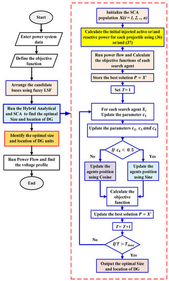
Figure 3.
Flowchart of the proposed hybrid analytical–SCA technique for the optimal DG allocation.
- Step 1
- Enter line and load data, and bus voltage limits.
- Step 2
- Determine the power losses using forward/backward load flow sweep.
- Step 3
- Specify candidate buses using LSF and the sizes of the DGs using the analytical technique for Type I using (36) and Type II using (37).
- Step 4
- Initialize the population of solutions using the values obtained from step 3 within the limits in the search space and set = 0.
- Step 5
- If the voltage values of all buses are within the constraint, estimate the power losses using (1). Otherwise, that solution is infeasible.
- Step 6
- Select the solution associated with the best objective function and set the value of the objective function as the current fitness function.
- Step 7
- Update the situation of the search agent using (42) and (43).
- Step 8
- If , go to step 9; otherwise, go to step 6.
- Step 9
- Print the results and optimal purpose position including the locations and sizes of various types of multiple numbers of the DGs and the corresponding optimal destination fitness, which represents minimum power losses.
4. Result and Discussion
In this work, two standard IEEE 33-bus and 69-bus systems are selected to check the performance of the proposed hybrid optimization algorithm. The base voltages and apparent power for all of them are 12.66 kV and 100 MVA. The developed approach has been programmed using MATLAB 2015, which runs on Intel core i5, processor 2.9 GHz PC with capacity 8.0 GB RAM and operates with Win.10. The following four cases are considered in the two studied systems with three types of the DGs (Type I, Type II, and Type III):
- Case 1: Base case (without DG).
- Case 2: Integrating one DG.
- Case 3: Integrating two DGs.
- Case 4: Integrating three DGs.
For all case studies, a forward–backward sweep load flow is adopted to obtain the voltage profile.
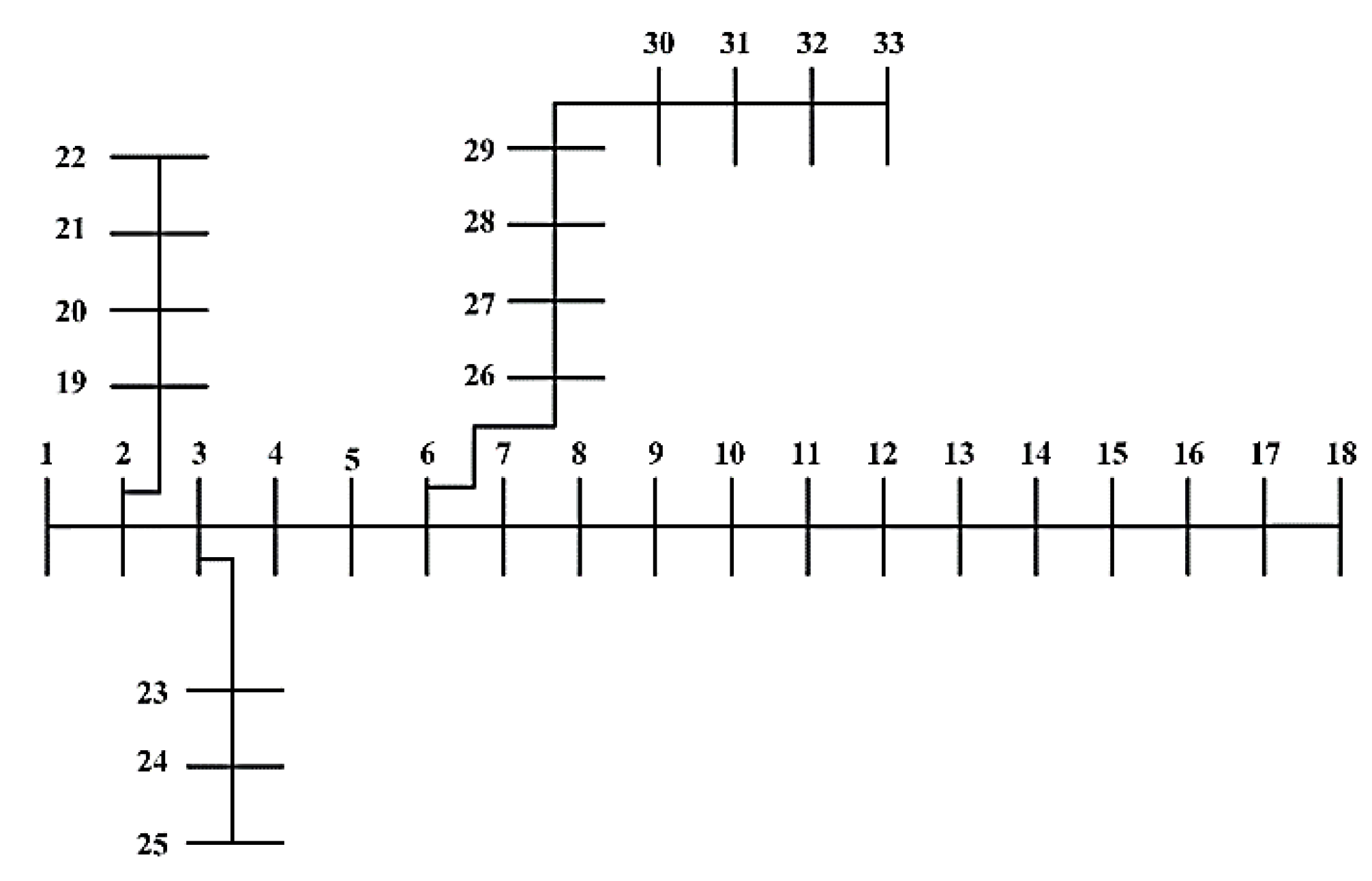
4.1. IEEE 33-Bus System
This system consists of 33 buses and 32 branches. The total active and reactive power loads are 3715 kW and 2300 kvar, respectively, as given in [28]. The single-line diagram is presented in Figure 4.
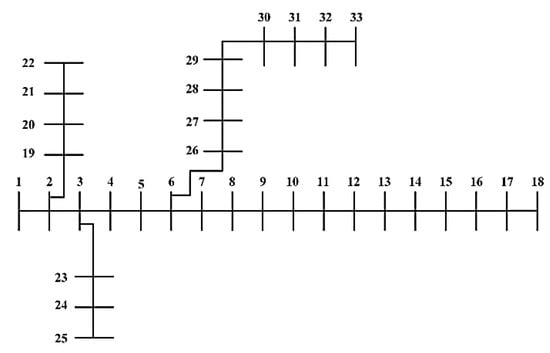
Figure 4.
Single line diagram of the IEEE 33-node test system.
4.1.1. Case 1: Base Case
In this case, the power losses before any compensation are 210.9862 kW and the minimum voltage is 0.9038 p.u at bus 18.
4.1.2. Case 2: Installing One DG
DG Type I
The power loss reduction of the proposed method and SCA is 47.381% and 47.381%, respectively, when the DG is placed on the same bus as described in Table 2. The size of the DG by hybrid technique is slightly higher than SCA. The power loss obtained by the proposed method is better than all other techniques.
Table 2.
Results of the hybrid approach and SCA with other techniques for Type I in IEEE 33-bus.
DG Type II
The power loss obtained by the proposed method and SCA is the same value, 28.258 kW, when the DG is placed at bus 30 for both of them with the nearly same size, and also they obtained the same minimum voltage value 0.9165 p.u at bus 18, as shown in Table 3, which also shows that the power loss obtained by the two approaches is better than 151.4 kW in hybrid PSO–analytical [25], 151.55 kW in the heuristic approach [29], and 164.6 kW in the analytical technique [10].
Table 3.
Results of the hybrid approach and SCA with other techniques for Type II in IEEE 33-bus.
DG Type III
Bus 6 is the best location for two approaches with the same power factor and nearly the same size, the power loss obtained for two approaches is 67.855 kW, as shown in Table 4, which is better than 82.78 kW in BSOA [15], 67.9 kW in the hybrid technique [30], and 81.43 kW in hybrid TLBO–GWO [23].
Table 4.
Results of the hybrid approach and SCA with other techniques for Type III in IEEE 33-bus.
4.1.3. Case 3: Installing Two DGs
DG Type I
The power loss reduction of the proposed method and SCA is 58.685% and 58.677% and the minimum voltage profile 0.9683 and 0.9680 p.u, respectively, with different sizes, as described in Table 2.
DG Type II
The power loss obtained by the proposed method and SCA is the same value 141.830 kW when the two DGs are placed at the same buses 12 and 30. Additionally, they obtained the same minimum voltage value 0.9303 p.u at bus 18, as shown in Table 3, which also shows that the power loss achieved by the two techniques is better than 143.84 kW in hybrid WIPSO–GSA [24], 141.9 kW in the heuristic approach [29], and 141.9 kW in the iterative–analytical method [9].
DG Type III
Buses 13, 30 are the best locations for the two approaches, but the power loss obtained by the hybrid technique is 28.5049 kW which is better than 29.2825 kW in SCA and also lower than all other techniques; 31.98 kW in BSOA [15], 29.33 kW in Hybrid WIPSO–GSA [24], 32.17 kW in hybrid TLBO–GWO [23], as shown in Table 4.
4.1.4. Case 4: Installing Three DGs
DG Type I
The power loss was reduced from 210.98627 kW to 72.789 kW for the proposed method which is less than 72.831 for SCA when the 3 DGs are placed at 13, 24, and 30 as shown in Table 2. Additionally, these values are lower than 89.90 kW in BFOA [32], 75.412 kW in KHA [21], 73.4 kW in BA [20], 77.06 kW in WOA [18], and 73.62212 kW in AIS [33].
DG Type II
The power loss for the proposed method is 138.260 kW, which is less than 138.600 kW for SCA when buses 13, 24, and 30 with sizes 396.103, 524.809, and 1044.227 kvar, respectively, are chosen as the best locations for the proposed method. However, SCA suggests buses 12, 24, and 30 as the best locations with the best sizes 427.400, 468.830, and 946.585 kvar, as described in Table 3.
DG Type III
Optimal power loss obtained in this case using the proposed method is 11.757 kW when three DGs are installed at buses 14, 24, and 30, while in the case of SCA, the power loss of the DGs placed at buses 12, 25, and 30 is 15 kW, as shown in Table 4.
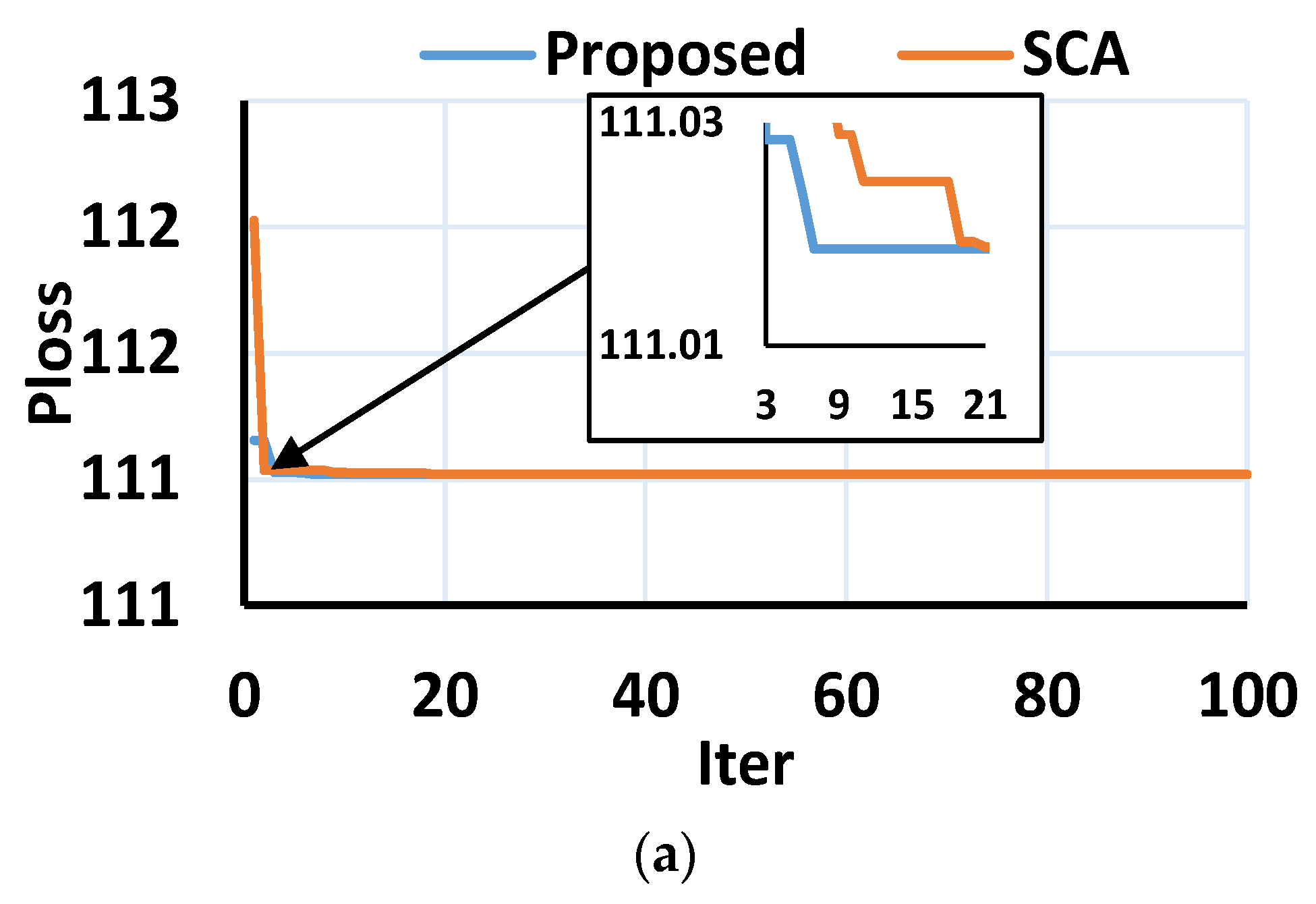
4.1.5. Performance Analysis for the Developed Technique
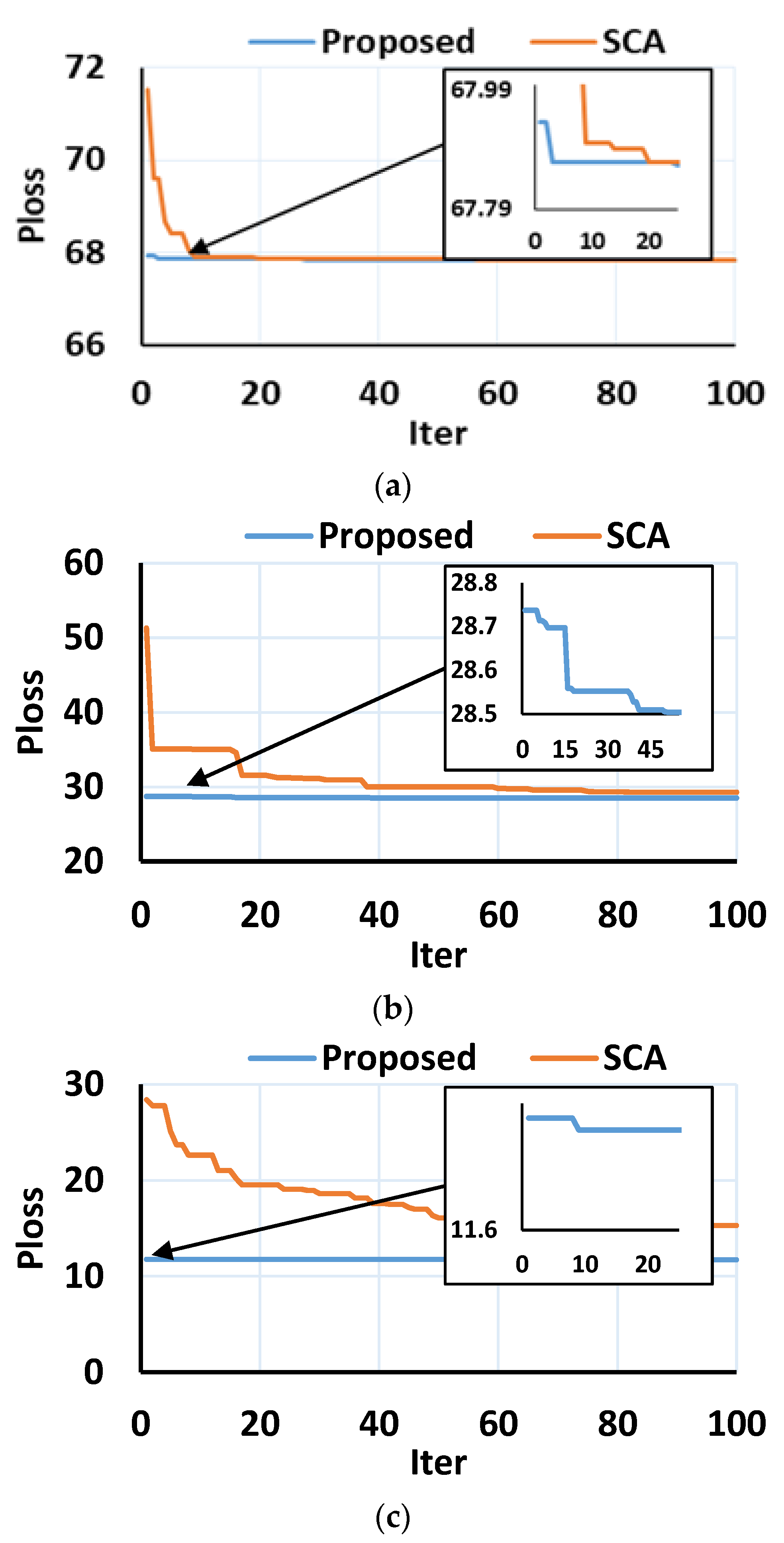
The convergence characteristics of the proposed method and SCA for Case 2, Case 3, and Case 4, which represent one, two, and three DG integration of Type I, have been illustrated in the Figure 5. The proposed hybrid technique obtains the minimum objective function in fewer iterations number compared with SCA. Figure 6 shows the high convergence rate achieved by the proposed method for one, two, and three DGs of Type II; Figure 7 also shows the comparison in the convergence curve between the proposed method and SCA to obtain minimum power losses.
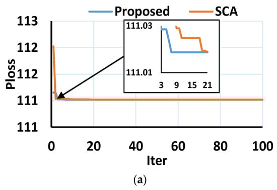
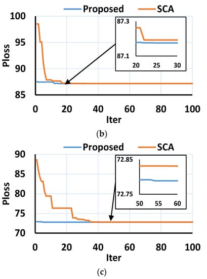
Figure 5.
Convergence curve for Type I DG integrating at different case studies in IEEE 33-bus. (a) Case 2, (b) Case 3, and (c) Case 4.

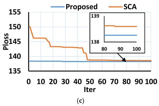
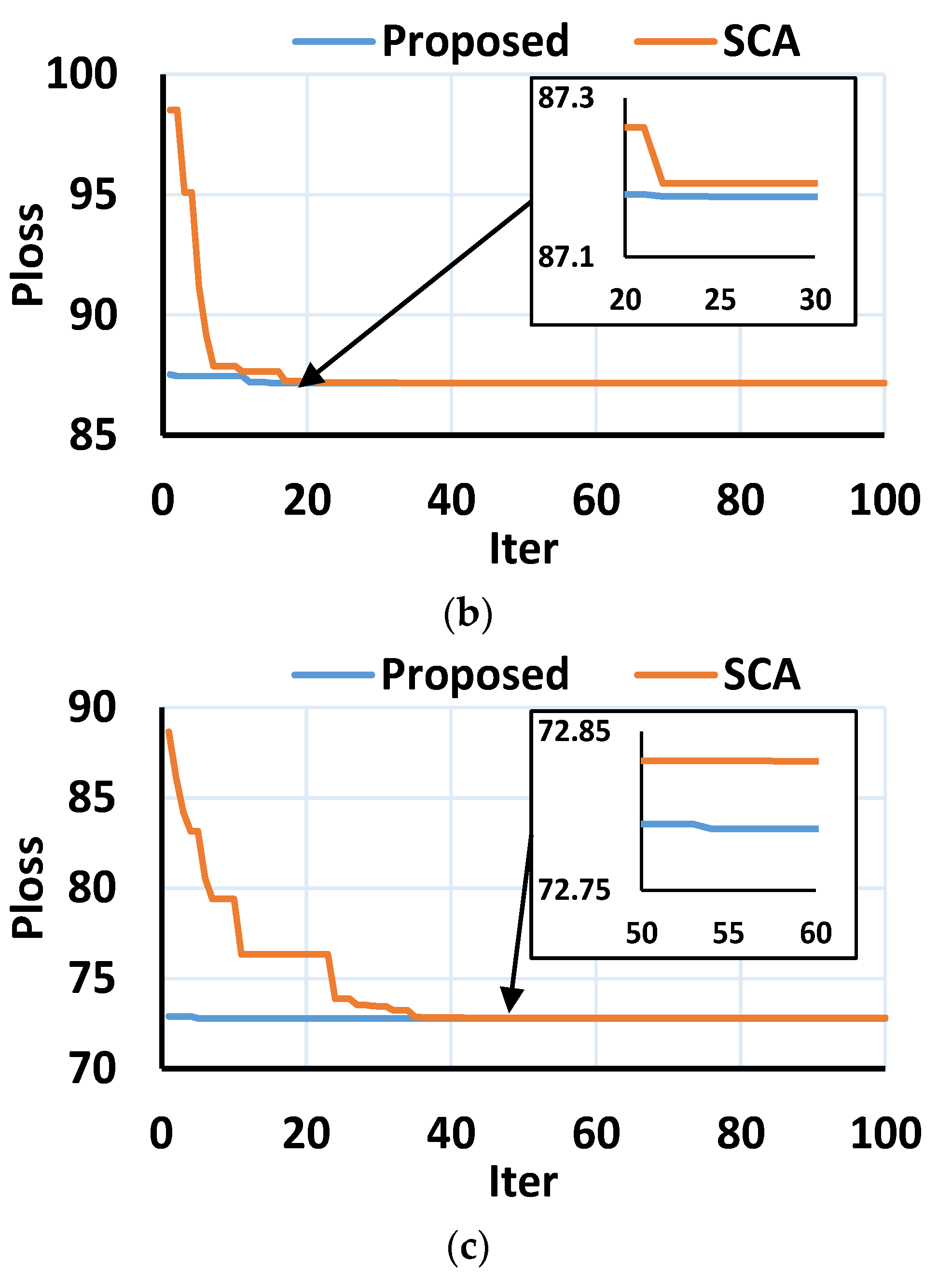
Figure 6.
Convergence curve for Type II DG integrating at different case studies in IEEE 33-bus. (a) Case 2, (b) Case 3, and (c) Case 4.
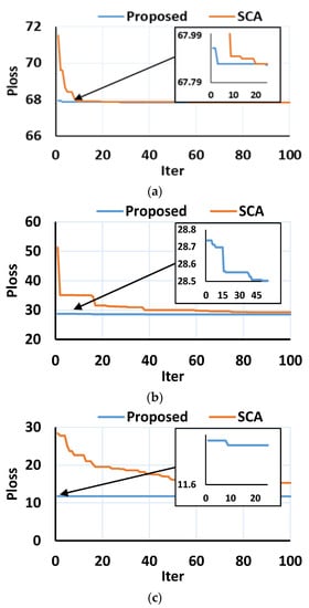
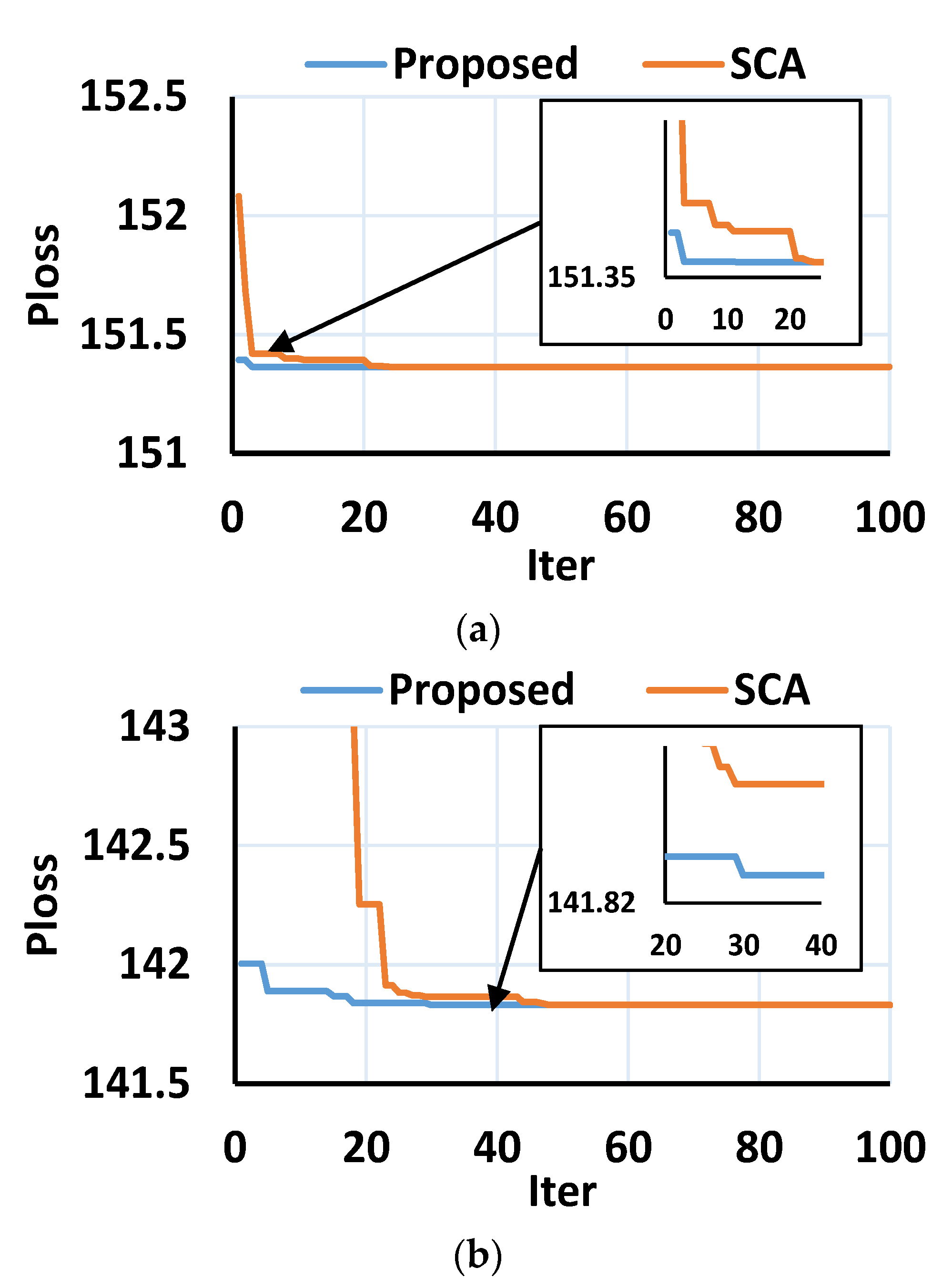
Figure 7.
Convergence curve for Type III DG integrating at different case studies in IEEE 33-bus. (a) Case 2, (b) Case 3, and (c) Case 4.
As observed in the figures, for one DG of Type I, Type II, and Type III, the convergence curve is slightly approximated, but in the case of more than one DG, there is a marked difference between the hybrid technique and SCA; hence, the proposed hybrid approach is an efficient method to solve multiple DG allocations problems in RDS.
In addition, Table 5 summarizes a comparison between the proposed algorithm and the original SCA in terms of computation time at the different case studies. The table proves that the average computation time and the standard deviation (STD) in the proposed algorithm are 63.68 and 2.09 s, which are lower than 70.61 and 3.27 s in the case of SCA.
Table 5.
Computation time (s) of the proposed algorithm compared to the SCA in IEEE 33-bus.
4.1.6. Voltage Profile
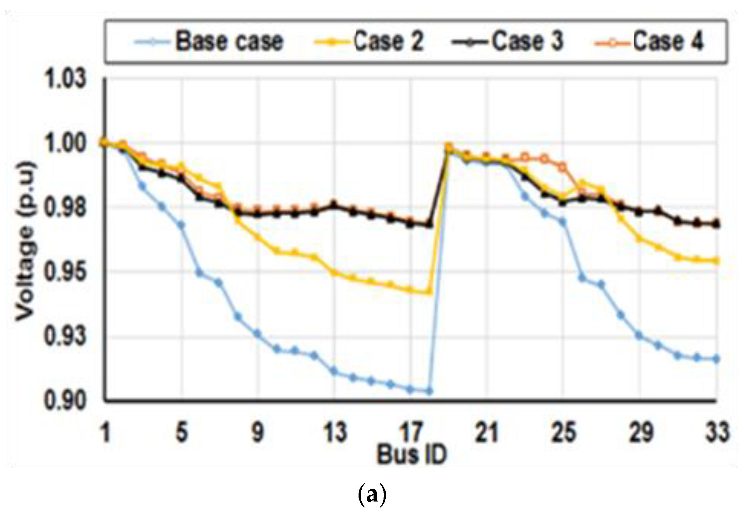
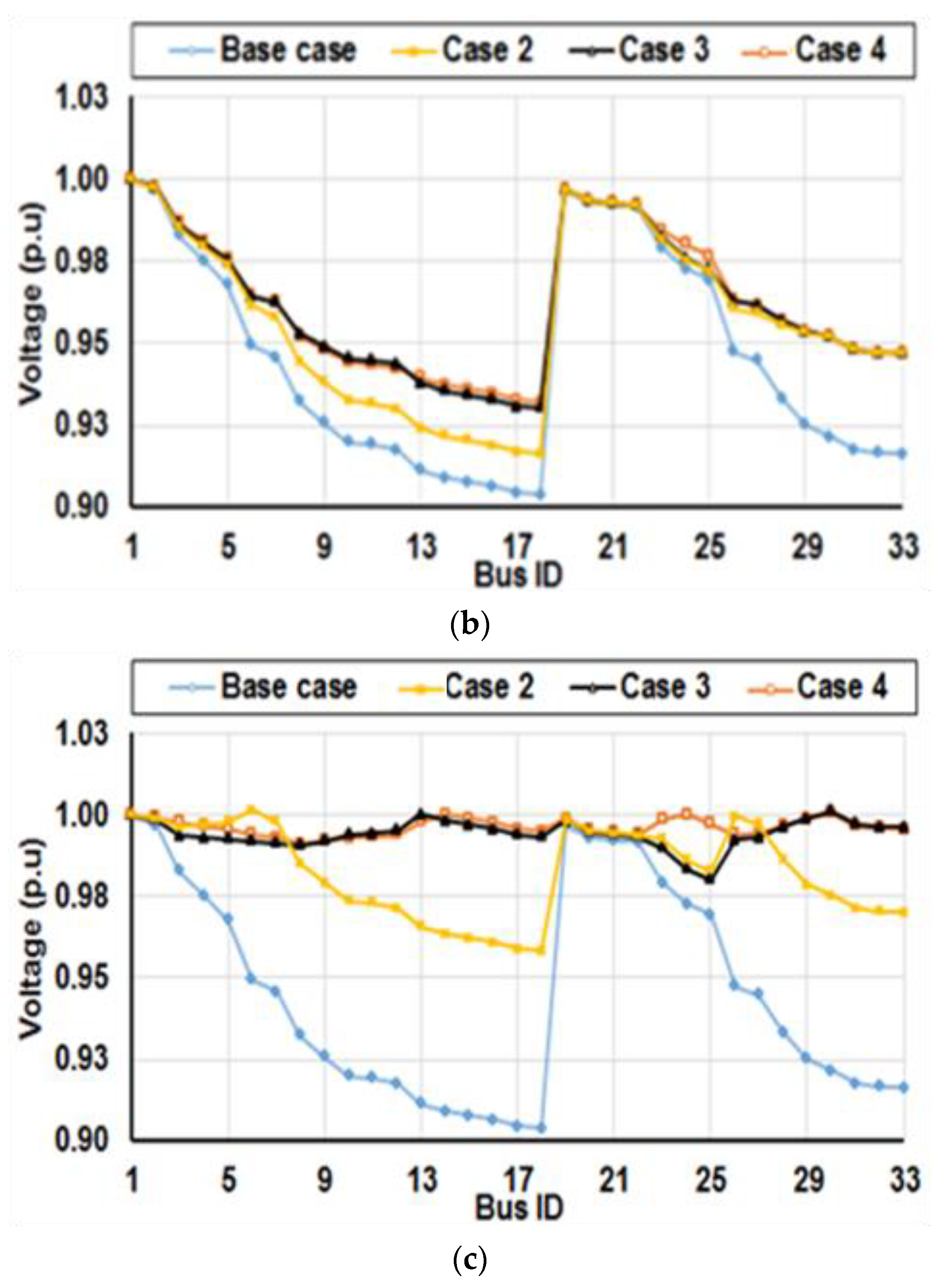
Figure 8 introduces the improvement in the voltage profiles of three types of DGs. It is clear that the minimum voltages are improved gradually with increasing the number of the DG integration. For DG Type I (see Figure 8a), Case 4 gives the best voltage profile compared to the other cases. However, the best improvement is achieved in the case of three Type III DGs, as shown in Figure 8c and assigned in Table 4.
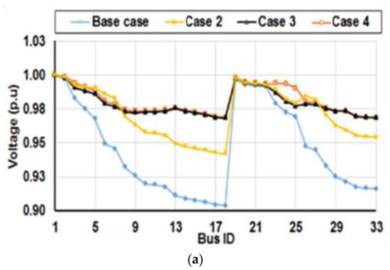
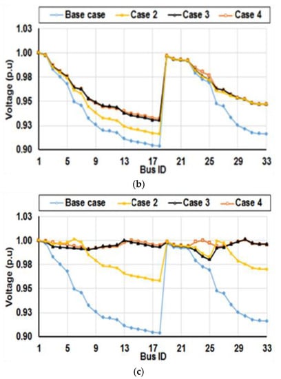
Figure 8.
Voltage profile of IEEE 33-bus with DG interacting at different DG types. (a) Type I, (b) Type II, and (c) Type III.
4.2. IEEE 69-Bus System
This system consists of 69 buses and 68 branches, as shown in Figure 9. The total active and reactive power loads are 3801 kW and 2690 kvar, respectively. The overall data of this system are given in [34].
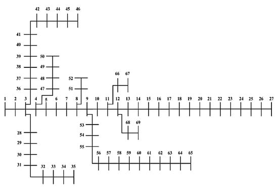
Figure 9.
Single line diagram of the IEEE 69-bus test system.
4.2.1. Case 1: Base Case
In this case, the power losses before any compensation are 224.9599 kW and the minimum voltage is 0.9092 p.u at bus 65.
4.2.2. Case 2: Installing One DG
DG Type I
The power loss reduction of the proposed method and SCA is 63.037% when the DG is placed at the 61 with size 1872.64 kW, And the minimum voltage is 0.9683 at bus 27 for both algorithms. This value of power loss reduction is better than 83.2231 kW in ALO [16], 111.56 kW in hybrid TLBO–GWO [23], 83.24 kW in GWO [17], and 83.21 kW in hybrid fuzzy–PSO [26], as described in Table 6.
Table 6.
Results of the hybrid approach and SCA with other techniques for Type I in IEEE 69-bus.
DG Type II
The power loss obtained by the proposed method and SCA is the same value, which equals 152.005 kW when the DG is placed at bus 61 with size 1329.93 kvar, and also they obtained the same minimum voltage value 0.9307 at bus 65, as shown in Table 7, which also shows that the power loss achieved by the proposed hybrid technique is less than 152.10 kW in the heuristic [29] and hybrid [25] approaches.
Table 7.
Results of the hybrid approach and SCA with other techniques for Type II in IEEE 69-bus.
DG Type III
Bus 61 is the best location for the proposed technique with the same power factor, but the size of the DG by SCA is slightly bigger than the size obtained by the proposed method; hence, the power loss obtained by the proposed technique is 23.13 kW, which is less than 23.17 kW in SCA, 58.80 kW in hybrid TLBO–GWO [23], 23.1622 kW in ALO [30], and 23.26 kW in EA [11], as shown in Table 8.
Table 8.
Results of the hybrid approach and SCA with other techniques for Type III in IEEE 69-bus.
4.2.3. Case 3: Installing Two DGs
DG Type I
The power loss for the proposed method when the DGs are placed at buses 17 and 61 with sizes 531.36 and 1781.47 kW, respectively, is 71.656 kW, which is slightly less than 71.774 kW in SCA and also better than 83.34 kW in hybrid TLBO–GWO [23], 71.74 kW in GWO [17], and 71.70 kW in hybrid fuzzy–PSO [26].
DG Type II
The power loss reduction obtained by the proposed method is 34.92%, which is slightly better than 34.91% obtained by SCA. Both of them select buses 17 and 61 as the best locations, as illustrated in Table 7, which shows the power loss reduction of the proposed method is higher than 34.88% for the iterative-analytical [9] and hybrid [25] methods.
DG Type III
Buses 17 and 61 are the best locations for the proposed technique; the power loss reduction obtained by the hybrid technique is 96.80%, which is higher than 96.09% in SCA and also better than 96.79% in the iterative-analytical method [9] and 90.69% in ALO [30], as described in Table 8.
4.2.4. Case 4: Installing Three DGs
DG Type I
The power loss was reduced from 224.9599 to 69.417 kW for the proposed method, which is less than 71.77 in SCA. Additionally, these values are less than 74.77 kW in PSO [19], 70.19 kW in WOA [18], 71.1 kW in DA [18], and 72.37 kW in MFO [19].
DG Type II
The power loss for the proposed method is 145.09 when three DGs are installed at buses 11, 21, and 61 which is better than 145.48 kW in SCA, 145.3 kW in the heuristic approach [29], 145.29 kW in the iterative–analytical method [9], and 145.26 kW in SSA [22], as shown in Table 7.
DG Type II
Optimal power loss obtained in this case using the proposed method is 4.2689 kW when three DGs are installed at buses 11, 18, and 61. This power loss is less than 7.089 kW obtained by WOA [18], 5.001 kW by DA [18], and 7.27 kW by hybrid TLBO–GWO [23], while in case of the SCA technique, the DGs are placed at buses 17, 49, and 61, and the power loss is 10.347 kW.
4.2.5. Performance Analysis for the Developed Technique
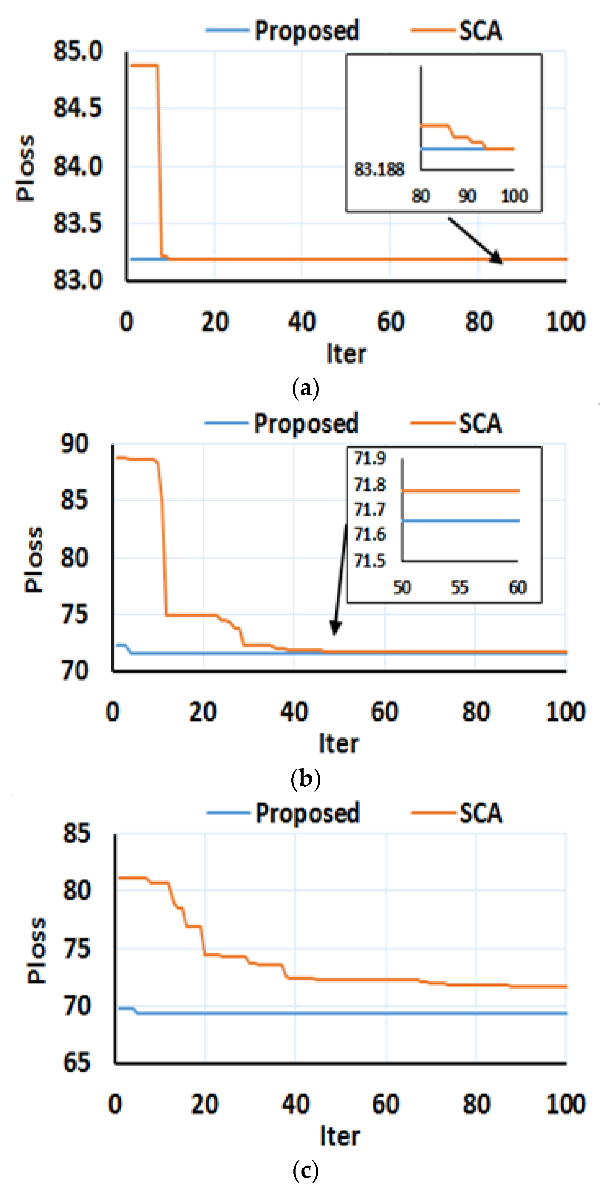
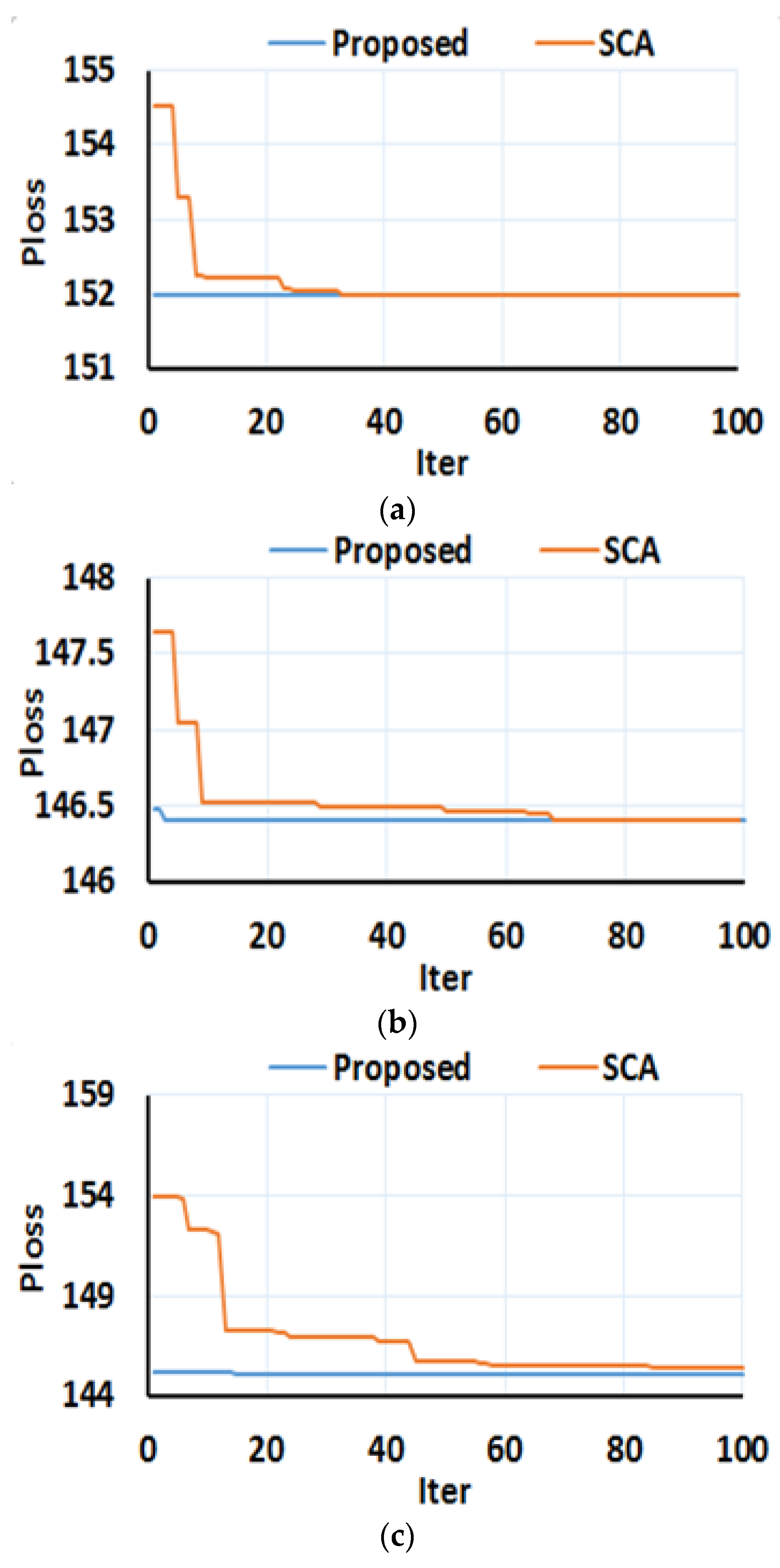
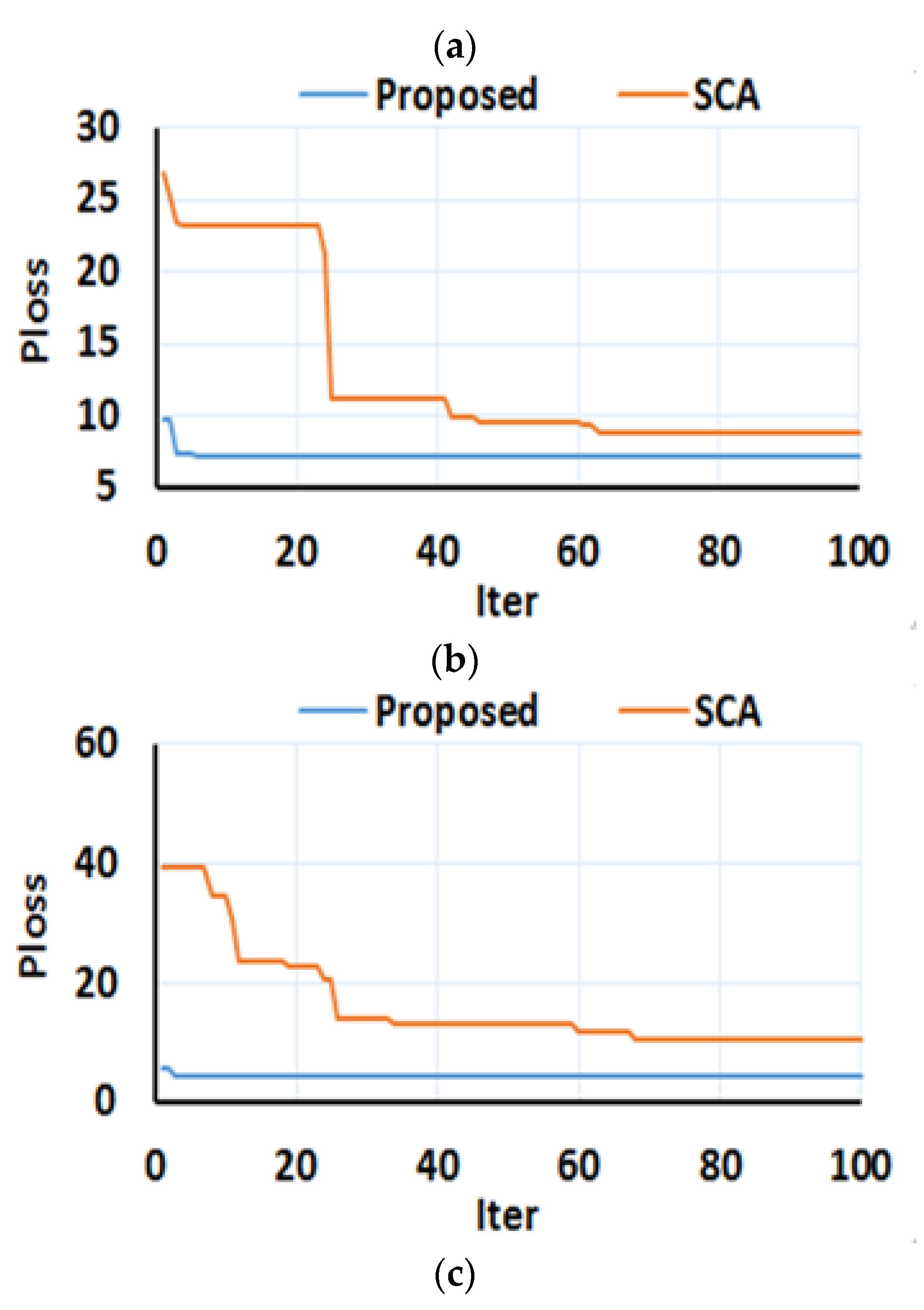
Similar to the IEEE 33-bus, the convergence characteristics of the proposed method and SCA for one, two, and three DGs of Type I are illustrated in Figure 10. The proposed hybrid technique gives the best result in a lower iteration number compared with SCA. Figure 11 shows the convergence characteristic obtained by the hybrid approach and SCA for Type II. Additionally, Figure 12 shows the convergence curve between the proposed method and SCA that gives the minimum objective function in Type III. The proposed method achieves the best results in the case of installing three DG in all DG types compared with SCA.
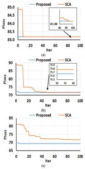
Figure 10.
Convergence curve for Type I DG integrating different case studies in the IEEE 69-bus. (a) Case 2, (b) Case 3, and (c) Case 4.
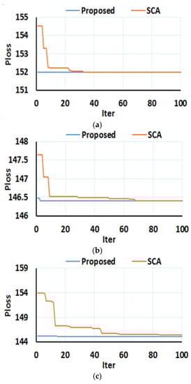
Figure 11.
Convergence curve for Type II DG integrating different case studies in the IEEE 69-bus. (a) Case 2, (b) Case 3, and (c) Case 4.
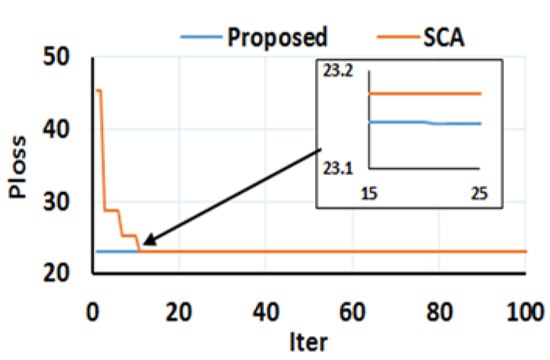
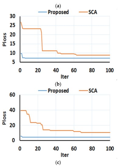
Figure 12.
Convergence curve for Type III DG integrating different case studies in the IEEE 69-bus. (a) Case 2, (b) Case 3, and (c) Case 4.
To prove the feasibility of the proposed algorithm, computation time is calculated at the different case studies and tabulated in Table 9. It is clear that the proposed algorithm is faster than the original SCA, where it recorded an average of computation time equal to 81.75 s with STD equal to 1.07 s, and that is better than 86.97 s and 3.25 s, which are given by SCA.
Table 9.
Computation time (s) of the proposed algorithm compared to the SCA in IEEE 69-bus.
4.2.6. Voltage Profile
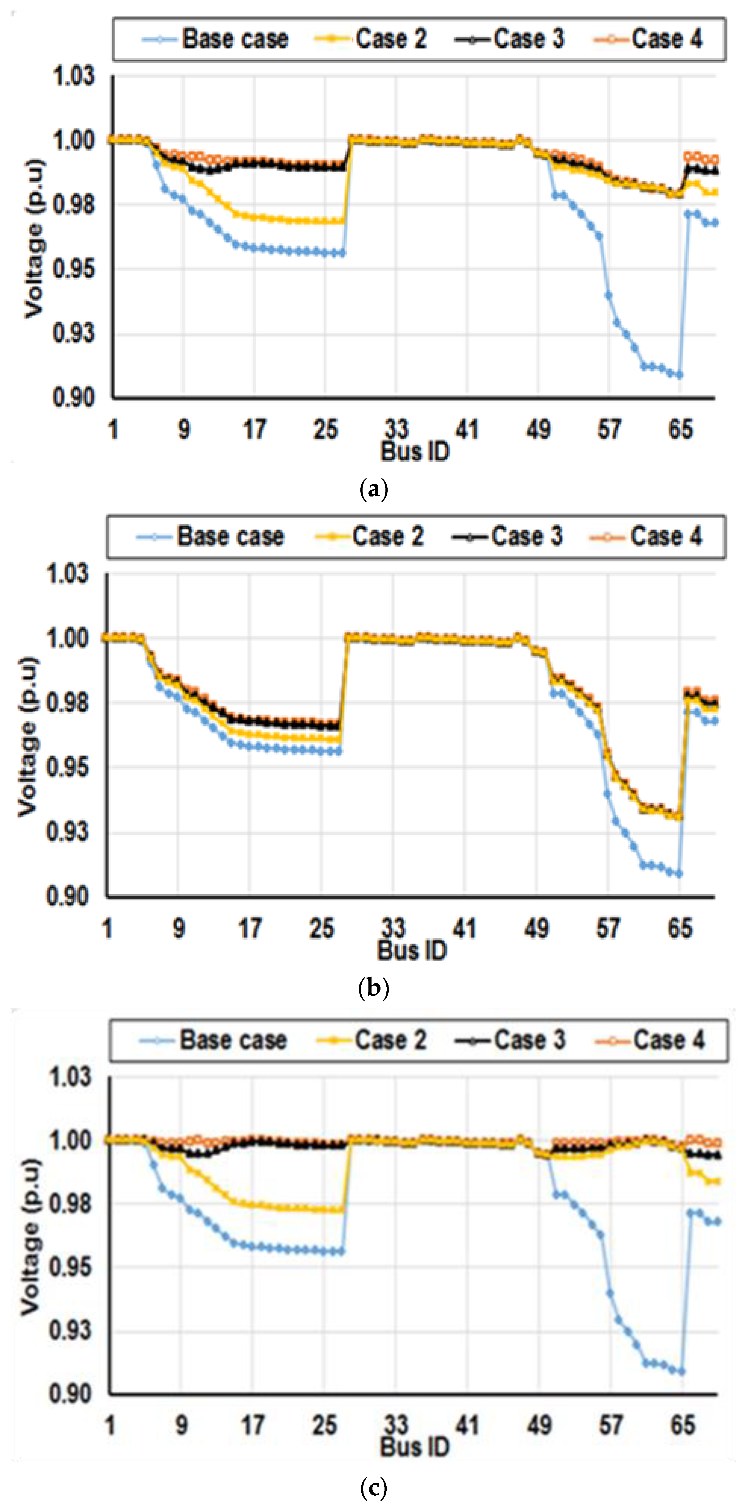
While Figure 13 introduces the voltage profiles improvement of Type I, Type II, and Type III for different case studies of multiple DG integration, it is clear that the voltage has been significantly increased when integrating three DGs from Type III, as shown in Figure 13c (Case 4), and that is because of the injection of active and reactive powers from the DGs.
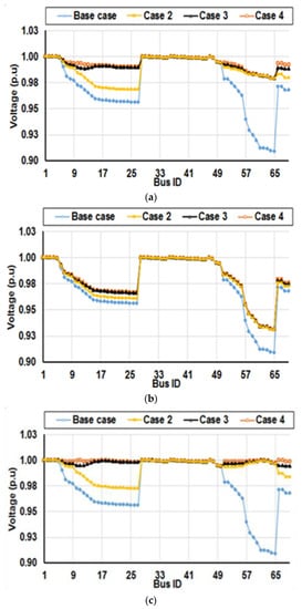
Figure 13.
Voltage profile of IEEE 69-bus with DG interacting in different DG types. (a) Type I, (b) Type II, and (c) Type III.
5. Conclusions
This paper has presented a hybrid optimization technique for optimal placement of multiple DGs with multiple types to minimize power losses and improve voltage profile. In the proposed hybrid technique, LSF with the fuzzy controller has been implemented to identify the candidates’ buses for the DG allocation. Then, the analytical technique based on the exact loss formula has been adopted to calculate the best sizes of the DGs. Finally, the candidates’ buses and the sizes have been used as initial values for the metaheuristic SCA to determine the final optimal sizes and the locations of the DGs in RDS. The proposed hybrid technique has been tested using two IEEE standard systems, 33-bus and 69-bus. Three DG types have been used in this work (Type I, Type II, and Type II). The proposed hybrid technique achieved the best results with fast convergence compared to the SCA and the other competitive optimization algorithms. The results show that a significant loss reduction has been achieved using the proposed method, which is equal to 94.43% and 98.10% when installing three DGs of Type III in the IEEE 33-bus and IEEE 69-bus, respectively. In addition, the voltage profile has been dramatically improved and reached 0.9912 p.u (at bus 8) and 0.9943 p.u (at bus 50) in the IEEE 33-bus and IEEE 69-bus, respectively, when installing three DGs of Type III. Hence, the results proved the ability of the proposed technique to allocate multiple DG units with different types into RDS.
Author Contributions
Conceptualization, A.A.M. and S.K.; data curation, A.S., E.E.E., and A.A.M.; formal analysis, S.K.; resources, A.A.M.; methodology, A.S. and E.E.E.; software, A.A.M., S.K. and A.S.; supervision, S.K. and E.E.E.; validation, A.S.; visualization, A.A.M. and E.E.E.; writing—original draft, A.A.M. and A.S.; writing—review and editing, S.K. and E.E.E. All authors together organized and refined the manuscript in the present form. All authors have read and agreed to the published version of the manuscript.
Funding
This work was supported by Taif University Researchers Supporting Project number (TURSP-2020/86): Taif University, Taif, Saudi Arabia.
Institutional Review Board Statement
Not applicable.
Informed Consent Statement
Not applicable.
Data Availability Statement
Not applicable.
Conflicts of Interest
The authors declare no conflict of interest.
References
- Singh, D.; Misra, R.; Singh, D. Effect of load models in distributed generation planning. IEEE Trans. Power Syst. 2007, 22, 2204–2212. [Google Scholar] [CrossRef]
- El-Samahy, I.; El-Saadany, E. The effect of DG on power quality in a deregulated environment. In Proceedings of the IEEE Power Engineering Society General Meeting, San Francisco, CA, USA, 12–16 June 2005; IEEE: Piscataway, NJ, USA, 2005; pp. 2969–2976. [Google Scholar]
- Ackermann, T.; Andersson, G.; Söder, L. Distributed generation: A definition. Electr. Power Syst. Res. 2001, 57, 195–204. [Google Scholar] [CrossRef]
- Marwali, M.N.; Jung, J.-W.; Keyhani, A. Stability analysis of load sharing control for distributed generation systems. IEEE Trans. Energy Convers. 2007, 22, 737–745. [Google Scholar] [CrossRef]
- Prakash, P.; Khatod, D.K. Optimal sizing and siting techniques for distributed generation in distribution systems: A review. Renew. Sustain. Energy Rev. 2016, 57, 111–130. [Google Scholar] [CrossRef]
- HA, M.P.; Huy, P.D.; Ramachandaramurthy, V.K. A review of the optimal allocation of distributed generation: Objectives, constraints, methods, and algorithms. Renew. Sustain. Energy Rev. 2017, 75, 293–312. [Google Scholar]
- Mohamed, A.A.; Kamel, S.; Selim, A.; Khurshaid, T.; Rhee, S.-B. Developing a Hybrid Approach Based on Analytical and Metaheuristic Optimization Algorithms for the Optimization of Renewable DG Allocation Considering Various Types of Loads. Sustainability 2021, 13, 4447. [Google Scholar] [CrossRef]
- Hung, D.Q.; Mithulananthan, N. Multiple distributed generator placement in primary distribution networks for loss reduction. IEEE Trans. Ind. Electron. 2013, 60, 1700–1708. [Google Scholar] [CrossRef]
- Forooghi Nematollahi, A.; Dadkhah, A.; Asgari Gashteroodkhani, O.; Vahidi, B. Optimal sizing and siting of DGs for loss reduction using an iterative-analytical method. J. Renew. Sustain. Energy 2016, 8, 055301. [Google Scholar] [CrossRef]
- Naik, S.G.; Khatod, D.; Sharma, M. Optimal allocation of combined DG and capacitor for real power loss minimization in distribution networks. Int. J. Electr. Power Energy Syst. 2013, 53, 967–973. [Google Scholar] [CrossRef]
- Mahmoud, K.; Yorino, N.; Ahmed, A. Optimal distributed generation allocation in distribution systems for loss minimization. IEEE Trans. Power Syst. 2015, 31, 960–969. [Google Scholar] [CrossRef]
- Naik, S.N.G.; Khatod, D.K.; Sharma, M.P. Analytical approach for optimal siting and sizing of distributed generation in radial distribution networks. IET Gener. Transm. Distrib. 2014, 9, 209–220. [Google Scholar] [CrossRef]
- Selim, A.; Kamel, S.; Jurado, F. Optimal allocation of distribution static compensators using a developed multi-objective sine cosine approach. Comput. Electr. Eng. 2020, 85, 106671. [Google Scholar] [CrossRef]
- Ehsan, A.; Yang, Q. Optimal integration and planning of renewable distributed generation in the power distribution networks: A review of analytical techniques. Appl. Energy 2018, 210, 44–59. [Google Scholar] [CrossRef]
- El-Fergany, A. Optimal allocation of multi-type distributed generators using backtracking search optimization algorithm. Int. J. Electr. Power Energy Syst. 2015, 64, 1197–1205. [Google Scholar] [CrossRef]
- Ali, A.H.; Youssef, A.-R.; George, T.; Kamel, S. Optimal DG allocation in distribution systems using Ant lion optimizer. In Proceedings of the 2018 International Conference on Innovative Trends in Computer Engineering (ITCE), Aswan, Egypt, 19–21 February 2018; IEEE: Piscataway, NJ, USA, 2018; pp. 324–331. [Google Scholar]
- Sobieh, A.; Mandour, M.; Saied, E.M.; Salama, M. Optimal number size and location of distributed generation units in radial distribution systems using Grey Wolf optimizer. Int. Electr. Eng. J 2017, 7, 2367–2376. [Google Scholar]
- Saleh, A.A.; Mohamed, A.-A.A.; Hemeida, A. Optimal Allocation of Distributed Generations and Capacitor Using Multi-Objective Different Optimization Techniques. In Proceedings of the 2019 International Conference on Innovative Trends in Computer Engineering (ITCE), Aswan, Egypt, 2–4 February 2019; IEEE: Piscataway, NJ, USA, 2019; pp. 377–383. [Google Scholar]
- Saleh, A.A.; Mohamed, A.-A.A.; Hemeida, A.M.; Ibrahim, A.A. Comparison of different optimization techniques for optimal allocation of multiple distribution generation. In Proceedings of the 2018 International Conference on Innovative Trends in Computer Engineering (ITCE), Aswan, Egypt, 19–21 February; IEEE: Piscataway, NJ, USA, 2018; pp. 317–323. [Google Scholar]
- Yuvaraj, T.; Devabalaji, K.; Ravi, K. Optimal Allocation of DG in the Radial Distribution Network Using Bat Optimization Algorithm. In Advances in Power Systems and Energy Management; Springer: Berlin/Heidelberg, Germany, 2018; pp. 563–569. [Google Scholar]
- Sultana, S.; Roy, P.K. Krill herd algorithm for optimal location of distributed generator in radial distribution system. Appl. Soft Comput. 2016, 40, 391–404. [Google Scholar] [CrossRef]
- Sambaiah, K.S.; Jayabarathi, T. Optimal allocation of renewable distributed generation and capacitor banks in distribution systems using Salp Swarm algorithm. Int. J. Renew. Energy Res. 2019, 9, 96–107. [Google Scholar]
- Nowdeh, S.A.; Davoudkhani, I.F.; Moghaddam, M.H.; Najmi, E.S.; Abdelaziz, A.Y.; Ahmadi, A.; Razavi, S.; Gandoman, F.H. Fuzzy multi-objective placement of renewable energy sources in distribution system with objective of loss reduction and reliability improvement using a novel hybrid method. Appl. Soft Comput. 2019, 77, 761–779. [Google Scholar] [CrossRef]
- Rajendran, A.; Narayanan, K. Optimal multiple installation of DG and capacitor for energy loss reduction and loadability enhancement in the radial distribution network using the hybrid WIPSO–GSA algorithm. Int. J. Ambient Energy 2018, 41, 129–141. [Google Scholar] [CrossRef]
- Bala, R.; Ghosh, S. Applications, Optimal position and rating of DG in distribution networks by ABC–CS from load flow solutions illustrated by fuzzy-PSO. Neural Comput. 2019, 31, 489–507. [Google Scholar] [CrossRef]
- Kansal, S.; Kumar, V.; Tyagi, B. Hybrid approach for optimal placement of multiple DGs of multiple types in distribution networks. Int. J. Electr. Power Energy Syst. 2016, 75, 226–235. [Google Scholar] [CrossRef]
- Mirjalili, S. SCA: A sine cosine algorithm for solving optimization problems. Knowl.-Based Syst. 2016, 96, 120–133. [Google Scholar] [CrossRef]
- Baran, M.E.; Wu, F.F. Network reconfiguration in distribution systems for loss reduction and load balancing. IEEE Trans. Power Deliv. 1989, 4, 1401–1407. [Google Scholar] [CrossRef]
- Bayat, A.; Bagheri, A. Optimal active and reactive power allocation in distribution networks using a novel heuristic approach. Appl. Energy 2019, 233, 71–85. [Google Scholar] [CrossRef]
- Ali, E.; Elazim, S.A.; Abdelaziz, A. Ant Lion Optimization Algorithm for optimal location and sizing of renewable distributed generations. Renew. Energy 2017, 101, 1311–1324. [Google Scholar] [CrossRef]
- Kashyap, M.; Mittal, A.; Kansal, S. Optimal Placement of Distributed Generation Using Genetic Algorithm Approach. In Proceeding of the Second International Conference on Microelectronics, Computing & Communication Systems (MCCS 2017); Springer: Singapore, 2019; pp. 587–597. [Google Scholar]
- Kowsalya, M. Optimal size and siting of multiple distributed generators in distribution system using bacterial foraging optimization. Swarm Evol. Comput. 2014, 15, 58–65. [Google Scholar]
- Meera, P.; Hemamalini, S. Optimal siting of distributed generators in a distribution network using artificial immune system. Int. J. Electr. Comput. Eng. 2017, 7, 641. [Google Scholar]
- Baran, M.; Wu, F.F. Optimal sizing of capacitors placed on a radial distribution system. IEEE Trans. Power Deliv. 1989, 4, 735–743. [Google Scholar] [CrossRef]


Publisher’s Note: MDPI stays neutral with regard to jurisdictional claims in published maps and institutional affiliations. |
© 2021 by the authors. Licensee MDPI, Basel, Switzerland. This article is an open access article distributed under the terms and conditions of the Creative Commons Attribution (CC BY) license (https://creativecommons.org/licenses/by/4.0/).