Abstract
All of the possible strategies to reduce water losses in piped distribution systems follow the law of diminishing returns: the higher the expenditure on water loss reduction, the lower the progressive return in terms of water saved. Therefore, water utilities need to estimate the economic level of water losses (ELWL) so that they can reduce their water loss to the level where the cost to reduce the water losses is equal to the value of the water saved. This paper aims to estimate the ELWL using four different methods: the total cost method, the marginal cost method, the cumulative cost–benefit method, and the component-based methods. This analysis is based on data (2011–2016) on the water utilities of the city of Malang (PDAM Kota Malang), Indonesia. It was found that the total cost and marginal cost methods gave almost similar results for ELWL. However, the total cost method is preferred to calculate ELWL because it is the most accurate, easier to apply, and does not need a long data series. In addition, the estimated ELWL for PDAM Kota Malang was 21.76%, which is 3.71% higher than the water loss level estimated in 2016, which means that their strategies to reduce water loss are not cost-efficient. Moreover, the lack of data is a major challenge in the estimation of ELWL in Indonesia. This study emphasizes the importance of estimating the ELWL so that water utilities, especially in Indonesia, can evaluate their strategies in reducing water loss and improving their cost-effectiveness.
1. Introduction
Increasing water-use efficiency by 2030 is part of Sustainable Development Goal 6.4 [1]. This issue will become more important in the future, as the water demand is growing significantly, while water availability is shrinking, the cost of water treatment is increasing and water supply infrastructures are deteriorating [2]. In the upcoming 50 years, the global water demand is predicted to rise by 400% in several sectors [3]. As a result, many countries are expected to face water scarcity [4].
One of the ways to achieve water-use efficiency is by minimizing water losses in the water supply distribution networks [5]. Water loss is the part of system input volume (SIV) that is not billed and does not produce revenue, and it is equivalent to the difference between the SIV and authorized consumption [6]. Water losses can come from leakages in the distribution system, unauthorized water use, or error in the measuring equipment [7]. It is estimated that the global average water loss is 35%, while the average water loss in Indonesia is 32.75% [8].
Water loss is technically classified into real (leakage) and apparent losses [9]. The NRW (non-revenue water) comprises water losses and unbilled authorized consumption (Figure 1). The issue of apparent losses and unbilled authorized consumption are more apparent in developing countries, while developed countries mainly deal with leakage issues [10].
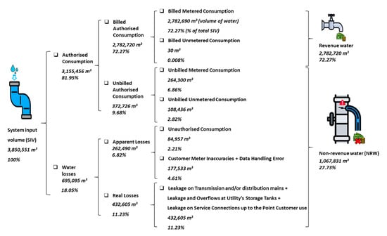
Figure 1.
Water balance of the water utilities of the city of Malang in October 2016 (source: PDAM Kota Malang).
The water losses lead to considerable financial loss for the water supplier. Globally, it was predicted that 126 billion m3 of water is lost every year, causing a financial loss of USD 39 billion per year [11].
Water loss reduction should be carried out to minimize the operating expenses (energy cost, maintenance cost and indirect cost) and increase the service level to the customer [12]. A fundamental fact about water loss reduction is that every possible reduction strategy follows the law of diminishing returns: the more the expenditure on water loss reduction, the less the returns in terms of water saved. Therefore, water utilities should aim to reduce their water loss to the economic level where the cost to carry out additional water loss control activity is equal to the cost of producing the water that could be saved from this additional leakage control activity [6,13].
Previous studies have focused on the calculation of the economic level of leakages (ELL) with different methods [14,15,16,17,18,19,20,21]. The calculation of ELL started in mid-1990 with the method known as the Total Cost method. At that time, the methodology focused on the minimum Total Cost Approach that would determine the economic frequency of the Active Leakage Control (ALC). Afterwards, in 2005, Lambert and Fantozzi [14] developed the formula for the economic intervention frequency based on the concept of the natural rate of the rising of unreported leakage. The second method is the marginal cost approach on the basis of the marginal cost of real loss reduction (the incremental annual cost of ALC intervention divided by the volume of water loss reduced in the same year) compared with the cost of producing additional water. The two-time frame approach was introduced by Pearson and Trow in 2005 [22], for the short-run and long-run of ELL. Lim et al. [15] developed the cumulative cost and benefit method, which determines the Economic Level of NRW based on the intersection between the cumulative cost curve and the cumulative benefits curve. A recent study introduced the concept of the Sustainable Economic Level of Leakage, which includes not only the long-term utility cost and benefits, but also the external social and environmental leakage cost, such as traffic commotion during pipe repair, the carbon footprint and health risk effects from leakages at low pressure [23]. A few studies tried to calculate the economic level of apparent losses (ELAL), but were limited only to calculating the optimum replacement frequency of water meters [24].
Many studies were focused on the ELL calculation, which only accounts for the economic level of real losses. However, there are a limited number of studies which try to determine the most economical value for total losses (real and apparent losses) called the economic level of water losses (ELWL), which uses a cost–effectiveness methodology. Previous studies used a cost–benefit methodology [25,26]. Moreover, there are no studies of ELL and ELWL in the water distribution system in Indonesia, and this paper aims to fill that gap.
The main objective of this paper is to quantify the ELWL. The ELWL can be obtained simply by adding up the ELL and ELAL values. However, in this study, different existing methods for the calculation of ELL were applied in order to determine the ELWL. In this study, four different methods were used to calculate ELWL: (i) the total cost method, (ii) the marginal cost method (iii) the cumulative cost–benefit method, and (iv) the component-based method. The results of those methods were compared, which provided some insights for the future calculation of the economic level of water losses. The municipal water utility (in Bahasa: Perusahaan Daerah Air Minum (PDAM) Kota Malang) of the city of Malang, Indonesia was used as a case study in this research.
2. Materials and Methods
2.1. Description of the Case Study
Malang is located in the province of East Java, Indonesia, with a total population of more than 800,000 inhabitants in 2015. The water supply in the city of Malang is provided by PDAM Kota Malang, a water company owned by the municipality of Malang. The total length of the distribution system at the end of 2016 was 3361.3 km. The service coverage at the end of 2015 was 84.61%. The water loss level was 20.42% and the NRW level was 28.96% in 2015 [27].
The data analyzed in the paper were collected between January and February 2017. We conducted the field data collection, gathered secondary data from several reports, such as technical report, financial report, and performance audit report, and also performed in-depth interviews with water company employees. Additionally, relevant information was collected, which included the monthly and yearly International Water Association (IWA) water balance (see for example Figure 1), costs related to water loss reduction, cost of production, water tariff, activity and procedure for active leakage detection, and meter inaccuracies for different ages of meters, etc. The data from the water utilities were available only from 2011 to 2016, which was used for the analysis.
2.2. Methods to Calculate the Economic Level of Water Losses (ELWL)
The four methods to calculate ELWL were compared: (1) the total cost method, (2) the marginal cost method, (3) the cumulative cost–benefit method, and (4) the component-based method. These four methods are usually used to calculate the ELL, and no study has estimated ELWL before, i.e., no method has been introduced to calculate ELWL. Therefore, we compare those methods to determine which method(s) is/are appropriate to estimate ELWL for our case study.
2.2.1. Total Cost Method
The total cost method was introduced in mid-1990 in England and Wales to calculate the ELL [28]. For a different level of physical losses, the annual cost of the water lost is summed up with the total cost of active leakage control in order to obtain the total cost curve. The lowest point on the total cost curve is considered to be the short-run ELL.
This total cost method will be used to calculate ELWL. The annual cost of lost water and the annual cost to reduce water loss are required to calculate the total cost. The annual cost of lost water is calculated from the water loss volume (not only the real loss) with this equation:
Cost of lost water = volume of water loss each year × water tariff
Meanwhile, the cost used yearly to reduce the water loss, namely the water loss control cost, consists of the investment cost and the yearly operational and maintenance cost. The investment cost—e.g., DMA establishment, meter replacement, and the installation of android software for meter reading—was spread to the annual cost based on their estimated lifetime. Three curves (the cost of the lost water, the water loss control cost, and the total cost) were plotted in a graph with cost as the Y-axis and the volume of water loss as the X-axis. The volume of water loss when the total cost is minimal is determined as the ELWL.
2.2.2. Marginal Cost Method
The marginal cost method is also often used in the United Kingdom as another method to calculate the Economic Level of Leakage [29]. In ELL estimation using this method, the marginal cost to obtain water from real loss reduction is compared with the cost of production. A similar concept was used for ELWL analysis: the marginal cost to obtain the additional water from the water loss reduction is compared with the marginal cost of producing additional water. The marginal cost to obtain the additional water from water loss reduction, namely the marginal cost of water loss reduction, is calculated with the following equation:
The calculation result of the marginal cost of water loss is then plotted to create the marginal cost curve, with the volume of the water loss as the X-axis. The ELWL on the X-axis is determined when the marginal cost of the water loss reduction is equal with the marginal cost of water. If the marginal cost for water loss reduction is lower than the marginal cost of water, it is better to reduce the water loss. In applying this method, the same data of the water loss control cost that is used in the total cost method is used to calculate the incremental cost for water loss reduction.
2.2.3. The Cumulative Cost–Benefit Method
The third method, the cumulative cost–benefit method, was the new method developed by Lim et al. [15], which was developed based on the particular operating conditions in South Korean water utilities. In this method, the relationship between the cumulative costs for water loss control is compared with the cumulative benefit of water loss reduction. The cumulative cost is derived from the annual cost for the reduction of the losses from water utilities. The annual benefit is calculated from the volume of water loss reduction each year multiplied by the marginal cost of water. The economic level of the water loss can be determined from the intersection of the cumulative cost curve and the cumulative benefit curve [15].
In this analysis, the cumulative cost was calculated from the same water loss control cost which was already counted in the total cost method section. In order to calculate the cumulative benefit, the water tariff is multiplied by the cumulative volume of the water loss reduction. The water loss reduction volume is calculated each year by deducting the volume of water loss in that year from the water loss volume in the previous year. The ELWL was identified by plotting the cumulative cost of water loss reduction curve and the cumulative benefit of water loss reduction curve together. In this case, the cumulative cost and cumulative benefit curve were plotted against the water loss/connection as the X-axis.
2.2.4. The Component-Based Method
In addition, for the ELWL calculation, the ELL and the ELAL were calculated separately in order to ascertain and compare the ELWL values resulting from the sum of the ELL and ELAL. The calculation of ELAL was conducted on meter replacement, which is directly related to economic meter inaccuracies [30]. The economic level of unauthorized consumption and the meter reading and billing error cannot be determined, as the data was not available. Therefore, ELWL was estimated as the total of ELL, the economic meter inaccuracies, the estimated volume of unauthorized consumption, and the meter reading and billing errors from the water balance. This approach is termed as “component-based method”.
The ELL was derived by comparing three methods: (1) the total cost method, (2) the marginal cost method, and (3) the cumulative cost–benefit method, i.e., similar to the calculation of ELWL. The procedure of determining ELL was the same as that explained above for the calculation of the ELWL. The difference is that the cost data used are directly related to the reduction of physical losses only. The cost to reduce real losses for five years was calculated based on data from fieldwork to create the real loss reduction cost curve. The cost of the water lost was obtained by multiplying the volume of real losses by the average cost of production.
Based on data availability, the ELAL analysis was conducted on meter replacement. Meter replacement is directly related to meter inaccuracies. The economic level of meter inaccuracies concerns when the meter is replaced in the most economical period, so that the annual cost for the meter is minimal. This level is affected by the accuracy of the old meter, the investment cost of the meter and the water tariff.
The annual cost of the meter was calculated by dividing the value of replacing the meter with the number of years the meter was installed. When the meters are replaced very quickly, the annual cost will be very high, and vice versa. The weighted error of the meter was used to calculate the cost of lost water from meter inaccuracies in that year. The cost of the lost water was calculated by multiplying the weighted error by the average consumption per year and the water tariff. The annual cost of lost water was calculated from the cumulative cost of lost water until that year divided by the number of years. When the meters are old, their weighted error becomes high and the annual cost of lost water will approach the annual cost of the meter.
2.3. Data Analysis
In order to generate the equation of the curve and extrapolate the curve for the total cost method, the power equation in Microsoft Excel was used, as suggested by the Tripartite group [31] and Lim et al. [15]. Based on the best practice principles of ELL calculation [31], the form of the real loss control cost curve could be log (raised to power), power, or a hyperbola. It was decided to use the power equation after considering the R2 of the other two curves. There are two main considerations in the assessment of the method’s performance: (1) whether the method is able to give results considering the limited data in our study case, and (2) the best fit to the data shown by the R2 of the equation [15].
The investment cost was spread to the annual investment annual cost based on the equipment lifespan. The lifespan considered is different for each type of equipment. For the DMA, the lifetime was estimated from the equipment with the highest cost (PRV), i.e., 5 years. The leakage detection equipment’s lifetime was estimated to be 10 years.
Finally, a sensitivity analysis was performed in order to ascertain which factors would have the most impact on ELWL, ELL and ELAL. The three parameters changed to analyze the ELWL sensitivity were: (i) the water tariff, (ii) the cost of production/marginal cost of water, and (iii) the water loss control cost. In ELL sensitivity, the cost of production and the real loss control cost were altered. Meanwhile, the water tariff and the cost of the meter were modified in order to ascertain the impact to ELAL. The purpose of the sensitivity analysis was to understand the most influential variable on the estimation of water losses. While performing the sensitivity analysis, only one parameter was varied and the other two parameters were kept constant. The parameter values were varied by −20%, −10%, +10%, and +20%, and the results obtained were compared with the baseline results.
3. Results
3.1. Calculation of the Economic Level of Water Losses (ELWL)
3.1.1. Total Cost Method
The water loss control cost, the cost of lost water and the total cost were plotted with the water loss/conn/year as the X-axis (Figure 2A). The five points were collected from the water utility data from 2011 to 2015. Figure 2A shows that the water loss control cost curve and the cost of lost water curve show a good fit for the data with high R2 in the power equation. Because the value of the total cost is still decreasing and the minimum value cannot be determined, all three curves need to be extended by applying the power equation (Figure 2B). From the extended curve and the calculation, the value of ELWL was obtained from the lowest total cost, i.e., at a water loss/conn of 67 m3/conn/year, or an estimated 21.76% of SIV (Figure 2B). The full calculation is shown in the Supplementary Materials S4.
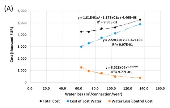
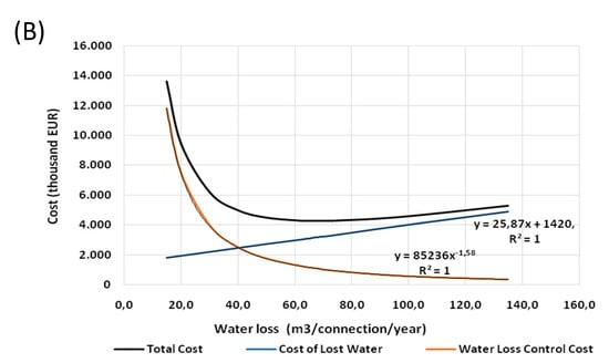
Figure 2.
(A) The ELWL curve from the water utility data; (B) the extrapolated ELWL.
3.1.2. Marginal Cost Method
As shown in Table 1, the volume of the water loss that can be reduced is smaller when the water loss level is lower but the incremental cost to reduce the water losses continues to increase. This results in the increasing value of the marginal cost of water loss reduction.

Table 1.
The marginal cost of water loss reduction.
The calculation result of the marginal cost of water loss reduction in 5 years (2011–2015) was plotted to create the marginal cost curve (Figure 3). The ELWL was determined when the marginal cost of water loss reduction was the same as the marginal cost of water. The cost of production and distribution, i.e., 0.26 EUR (conversion 1 EUR = 15.000 in March 2017), was used as the marginal cost of water. By using the formula of the curve, it was estimated that the ELWL was 67.76 m3/conn/year or 22.02% of the SIV. The estimated value of ELWL acquired from this method and the total cost method have slightly different results. This means that both the data and the method are reliable for ELWL estimation, i.e., considering the value of R2.
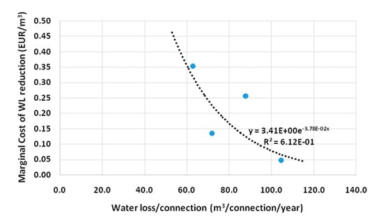
Figure 3.
The marginal cost curve for ELWL estimation.
3.1.3. Cumulative Cost and Benefit Method
Figure 4 shows that the cumulative cost and cumulative benefit curve has the best fit of data compared with the total cost and marginal cost method, i.e., the highest R2. There were four data points in the curves which were obtained from the water loss reduction data over the previous year, i.e., five years of data result in four data points. However, Figure 4 shows that the curves do not intersect each other and, thus, the ELWL could not be identified.
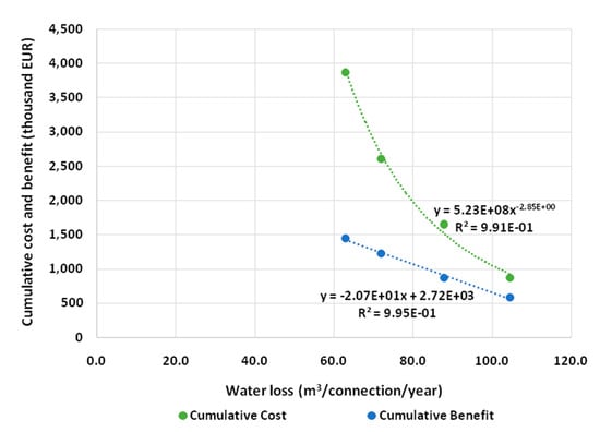
Figure 4.
The cumulative cost–benefit curve.
3.1.4. Component-Based Method
Figure 5A presents the real loss reduction cost, cost of water lost from leakage, and total cost from the water utility data (2011 to 2015). Figure 5B shows the calculated ELL at the volume of real losses of 4,604,143 m3/year, or 10.66% of the SIV. The marginal cost method was also applied to estimate ELL. However, the marginal cost curve derived from the data has a very low R2 (0.0005), such that it is not reliable to determine ELL from that curve. The calculation of the cumulative cost for real loss was also attempted, and the cumulative benefit was determined by multiplying the cost of production with the cumulative volume of real loss reduction. Nevertheless, the same result was obtained as in the ELWL estimation; the curves (cumulative cost and cumulative benefit) did not intersect each other and the ELL could not be determined (see Supplementary Material S2). Therefore, only the results from the first method, i.e., the total cost method, were used.
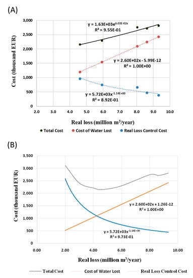
Figure 5.
(A). The ELL curve from the water utility data; (B) the extrapolated ELL.
For the ELAL analysis, the optimum meter replacement period was found to be 7 years (see Supplementary Material S3). The economic level of the meter inaccuracies was 1.41% of the billed metered consumption. Based on the percentage of the billed metered consumption, which was 70.84% of the SIV from the water balance in 2015, the economic meter inaccuracies were estimated as 0.99% of the SIV.
Unfortunately, it was not possible to calculate the other two components of ELAL: Unauthorized Consumption and Data Handling Error. Therefore, these values were estimated using the water balance in 2015. The estimated values of Unauthorized Consumption and Data Handling Error were 3.96 and 1% of the system input volume (SIV), respectively. The component-based method is theoretically the sum of ELL and ELAL. According to the results of ELL (10.66%) and ELAL (3.96% + 0.99% + 1%), the estimated ELWL was 16.61%.
3.2. Summary of the Methods
Table 2 presents a summary of the results. The total cost and marginal cost methods gave almost the same results, 21.76% and 22.02%, respectively, while the results of the component-based method were far below those of the other two methods, i.e., 16.61%. However, based on this analysis, the cumulative and cost benefits method could not be used in our case because the cumulative cost curve and cumulative benefit curve did not intersect.
Table 2.
Summary of the ELL, ELAL and ELWL results.
3.3. Sensitivity Analysis
3.3.1. Sensitivity Analysis for ELWL
- Total Cost Method
Both the water tariff and the water loss control cost influence the ELWL. When the water tariff is altered, the equation for the cost of the lost water is changed. The new equation is used to calculate the new cost of the water lost. On the other hand, when the water loss control cost is changed, the equation of the WL control cost also shifted and this equation is used to project the cost. Table 3 presents a summary of the changes in the water tariff and water loss control cost.
Table 3.
Sensitivity analysis of ELWL: the total cost method.
Table 3 shows that when the water tariff is increased, the ELWL will decrease. Additionally, there is an increase in the water loss control cost, resulting in a higher value of ELWL. However, when the water tariff and water loss control cost is altered at a similar value, the ELWL also changes at a similar rate. This means that there is no variable that most influences the ELWL value.
- ii.
- Marginal Cost Method
In this method, the different marginal cost of the water and the water loss control cost were also applied in order to ascertain the effect to the ELWL. When the marginal cost of the water loss control cost is changed, the value of ELWL can be estimated by using the same marginal cost curve. However, in order to apply the change of the WL control cost, the marginal cost curve needs to be created again for any changes. Table 4 shows the results of the sensitivity analysis with the marginal cost method. This result is almost similar to the result of the total cost method. This finding shows that the total cost method and marginal cost method will give almost-similar values of ELWL, although the water tariff is used in the total cost method and the marginal cost of water (the cost of production and distribution) is applied in the marginal cost method.
Table 4.
Sensitivity analysis of ELWL: the marginal cost method.
- iii.
- Cumulative Cost and Benefit Method
With the sensitivity analysis, it was found that the cumulative cost and cumulative benefit curve start to intersect when the marginal cost of water is increased to 160%. At this point, the ELWL will be 96 m3/conn/year. This is much higher than the result obtained from the other methods.
Another approach is to change the water loss control cost so that the cumulative cost decreases and intersects with the cumulative benefit curve. The cumulative cost and cumulative benefit curve meet when the water loss control cost decreases only by 5%. It is thus indicated that the modification of the cost of reducing water losses greatly affects the result of this method. For this option, the ELWL will be 83 m3/conn/year.
3.3.2. Sensitivity Analysis for ELL
- Total Cost Method
The sensitivity analysis for ELL was applied for the cost of production and the real loss control cost. One parameter was modified at a time while the other parameter was kept constant. Table 5 shows that when the cost of production is increased, the ELL value will be smaller. Furthermore, the reduction in the real loss control cost results in a lower value of ELL. When the cost of production and the real control cost was altered to a similar value, the ELL also changed at a similar rate. This means that there is no leading factor that controls the ELL value.
Table 5.
Sensitivity analysis of ELL: the total cost method.
- ii.
- Cumulative Cost and Benefit Method
The escalation of the cost of production by 60% will cause the cumulative cost and the cumulative benefit to start to intersect, at this point, and the ELL will be 65 m3/conn/year or 21.1% of the SIV. Similarly, the reduction of the real loss control cost by 35% causes both of the curves to meet; for this option, ELL will be 71 m3/conn/year or 23.06% of the SIV (see Supplementary Material S5). It can be concluded that alterations in the real loss control cost affect the ELL result more in the cumulative cost–benefit method.
3.3.3. Sensitivity Analysis for ELAL
Different water tariffs and costs of the water meters were applied to examine which factor affect economic meter inaccuracies value the most. When the water tariff is decreased, the annual cost of the water lost from meter inaccuracies will also decrease, and the annual cost of the meter dictates the economic meter replacement frequency. Because of that, the economic meter replacement frequency changes to 8 years and the economic meter inaccuracies increase to 2.18% (Table 6).
Table 6.
Sensitivity analysis for economic meter inaccuracies in PDAM Kota Malang.
Furthermore, the escalation in the cost of the meter also causes a higher annual cost of the meter. This annual cost then becomes the major parameter that determines the meter replacement frequency. The meter replacement frequency is changed to 8 years and the economic meter inaccuracies increase to 2.18%.
4. Discussion
Comparing all four methods, it was observed that the total cost method is the most applicable method to determined ELWL and ELL, i.e., it is able to estimate ELWL and also has a high R2. The marginal cost method needs a longer data series to produce a good fit (R2) value for the marginal cost curve, for which data availability is one of the issues in developing countries. For example, in this case, water utilities only have data for the last five years (2011–2015), and it was not possible to calculate the ELL with this method. The cumulative cost and benefits method gives good results in South Korean cases [15], but not in our case. This could be because PDAM Kota Malang spent too much money to reduce the water loss, such that the cumulative cost is far higher than the cumulative benefit. Moreover, the water tariff is also low, such that the cumulative benefit curve did not intersect with the cumulative cost curve.
The results of the component-based method are very different from the total cost and the marginal cost method. One of the possible reasons is because is also not possible in this case study to determine the ELAL of the unauthorised consumption and data handling error. The data from the water balance for both components were used to estimate ELWL. The data of the unauthorised consumption and the data handling error from the water balance are only based on technical judgement, not on real measurements, and so sometimes those data have a low level of accuracy.
In the sensitivity analysis for ELWL with the total cost and marginal cost methods, for three of the parameters altered (the water loss control cost, the water tariff and the cost of production), there was no variable that most influences the ELWL value. The same was true for the sensitivity analysis for ELL with both methods; changes in the real loss control cost or the marginal cost of water will affect the ELL value at a similar rate.
The sensitivity analysis for ELWL and ELL with the cumulative cost and benefits method showed that small changes in water loss control cost or real loss control cost will significantly affect the ELWL and ELL values. This means that this method is very sensitive to changes in the cost to reduce water loss. Hence, water utilities must be more careful in calculating the cost to obtain a good result from this method.
Based on the ELWL analysis, it was found that the ELWL is 21.76%, or 67 m3/conn/year. This is slightly higher than the water loss standard in Indonesia, i.e., it should be below 20% [32]. Considering the volume of water loss (18.05% in October 2016), the performance of the PDAM Kota Malang is relatively good. As a comparison, the average NRW in all of the water utilities in Indonesia is 37% [33], while in the city of Malang it is 27% (Table 1). However, if we look at the water balance data, the water loss of PDAM Kota Malang in 2016 was already below the ELWL, suggesting that the strategies of PDAM Kota Malang to reduce water loss are not cost-efficient. Therefore, it is recommended that PDAM Kota Malang should maintain the water loss at the economic level and avoid huge investment to decrease the water losses, i.e., they should re-think their current strategy.
Furthermore, the Economic Level of Leakage (ELL) and Economic Level of Water Losses (ELWL) in PDAM Kota Malang were compared with the ELL in Lembaga Air Perak, Malaysia [17] and ELWL in K-Water Korea [15]. In theory, when the cost of production is lower, the ELL or ELWL values should be higher and vice versa, but the reality based on this compilation is different. Although the Lembaga Air Perak has a lower cost of production (0.37 RM/m3 or 0.077 EUR/m3) than PDAM Kota Malang, the ELL in Lembaga Air Perak, Malaysia (17.88 L/conn/day) is lower than the ELL in PDAM Kota Malang (89.9 L/conn/day). PDAM Kota Malang, which has a lower cost of production than K-Water (1.51 £/m3 or 1.8 EUR/m3), has an ELWL (67 m3/conn/year) lower than the ELWL in K-Water Korea (132 m3/conn/year). This means that different methods and costs of reducing water losses in the different characteristics of the distribution system would result in different values of ELL and ELWL.
Analysing the economic level of water loss will not give accurate results if the water loss reduction strategy is not yet implemented, because the economic level is still far from being achieved and the data needed is not sufficient. The Infrastructure Leakage Index (ILI) can be used as an indicator for the utilities regarding whether they should assess the economic level or not. Farley and Liemberger [34] said that the economic level should be assessed for the waterworks in developing countries when their leakage performance category reaches band B (ILI < 8).
If the water utilities can estimate the economic level for each strategy of real loss (the active leakage control, pressure management, speed and quality of repair, and pipe and asset management) and apparent loss reduction (meter reading errors, water accounting errors, meters under registration, and water theft reduction) separately, they can set the prioritisation for the implementation of the strategy. However, the estimation of the economic level is highly dependent on the quality of the data. In some cases, it is challenging to measure the leakage reduction volume after each intervention. However, to assess the economic level for each strategy of real losses and apparent losses, this data is essential to predict the economic level. Every time an intervention is made to reduce water losses, the utilities should record the benefits gained, and also the costs. As an example, the pressure pattern before and after the PRV is installed should be recorded so that the volume of water saved after the pressure reduction can be estimated.
For the water utilities which have been successfully reducing the water losses continuously for several years and gathered the costs data that are directly related to the water loss reduction, it is recommended to apply all of the four methods to estimate the ELWL, even though one method was not applicable in our case. Those four methods can only be applied after the utilities continually decrease their water loss level from the higher level to the lower level for numerous years. However, if the water loss level for the utilities still varies and is not consistent, i.e., either decreasing or increasing suddenly, all of those methods will give an inaccurate result. This is because a positive value of the water loss reduction volume over the year is required to calculate ELWL.
The calculations of ELL and ELWL are determined by the rate of the renewal of assets. Asset renewal itself could be influenced by other factors besides leakage, such as a policy of the company on repair or replacement, the reliability of service, the rate of asset degradation, or the availability of financial resources. In this study case, PDAM Kota Malang could not afford to replace the pipes regularly according to their lifespan because of their limited budget. The water utilities replace the pipe but only for the pipe with the worst condition. This condition, known as a non-steady–state, could cause a drastic increase of the cost in maintaining water losses when the end of the life of the assets is near.
It was also pointed out that there is a need to calculate the ELWL or ELL in water utilities in Indonesia. The national target to reduce the water loss to 20% may create pressure on the water utilities to improve their distribution system. Considering the situation in PDAM Kota Malang, there is a high possibility that other water utilities will spend a lot of money for improvement without realising the economic benefits gained, i.e., following the law of diminishing returns [22]. However, we also realise that obtaining sufficient data for the ELWL and ELL calculation is an issue in Indonesia, i.e., there is a lack of data, or the water utilities did not properly collect the data. Therefore, we suggest an improvement of the data recording management in all water utilities (PDAM) in Indonesia, especially for the calculation of ELL and ELWL. This could lead to more cost-efficient strategies in reducing water loss.
We have several limitations in estimating the Economic Level of Water Losses. First, the dependency of the demand on the water price, i.e., when water prices increase, water demands decrease, which was not incorporated in this calculation. Second, due to data limitation mentioned in the previous paragraph, the R2 is quite low in Figure 3. More data points, instead of five points, i.e., 5 years, are also suggested to give more confidence in the regression results. Previous studies used five to seven data points to calculate NRW and ELL [15,35,36]. This implies that they faced the same issue of data availability.
5. Conclusions
This is the first study to estimate the ELWL by comparing four methods: (i) the total cost method, (ii) the marginal cost method, (iii) the cumulative cost–benefit method, and (iv) the component-based method. We found that the length of the data series will determine the accuracy of the results obtained from three of the methods (total cost, marginal cost, and cumulative cost-benefit). There is a limitation in the data availability, which makes it difficult to obtain reliable results using the cumulative cost–benefit and component-based methods. The total cost method is considered to be the best method for this case study. From the sensitivity analyses, it was found that in the case of the total cost and marginal cost methods, there is no variable that influences the calculation of ELL and ELWL significantly. However, the cumulative cost and benefit method is more sensitive to changes in the water loss control cost than total cost and the marginal cost methods. Therefore, the data required to be applied with this method should have higher accuracy than the other two methods. This study also revealed that even though PDAM Kota Malang has met the national standard of water losses, their current expenditure to reduce water loss is not cost-efficient. This study can be replicated by other water utilities in Indonesia to obtain the most economical target of water losses while reducing the water losses in their piped distribution systems. Finally, if sufficient data are available, we suggest estimating the economic level of water losses using all four methods in order to obtain a better insight into the economic aspects of water loss management and to reduce the errors associated with the assumptions in each method.
Supplementary Materials
The following are available online at https://www.mdpi.com/article/10.3390/su13126604/s1. S1: Cost for reducing real losses; S2: ELL Calculation; S3: ELAL Calculation; S4: ELWL Calculation; S5: Sensitivity Analysis.
Author Contributions
Conceptualization, T.H. and S.K.S.; methodology, T.H. and S.K.S.; software, T.H.; validation, T.H. and S.K.S.; formal analysis, T.H.; investigation, T.H.; resources, T.H.; data curation, T.H.; writing—original draft preparation, T.H. and D.D.; writing—review and editing, T.H., S.K.S., D.D. and M.K.; visualization, T.H. and D.D.; supervision, S.K.S. and M.K.; project administration, T.H.; funding acquisition, T.H. All authors have read and agreed to the published version of the manuscript.
Funding
The first author received funding from the StuNed (Studeren in Netherland) for Master’s study and thesis data collection.
Institutional Review Board Statement
Not applicable.
Informed Consent Statement
Not applicable.
Data Availability Statement
The data is contained within the article or Supplementary Material.
Acknowledgments
We thank President Director of PDAM Kota Malang (H. M Jemianto), the NRW division (Suwito, Gigih, Asvi, Desi, Farida, Andri), and the related division members that assisted in the data collection.
Conflicts of Interest
The authors declare no conflict of interest.
References
- United Nations. Sustainable Development Goal 6: Synthesis Report on Water and Sanitation; UN-Water: New York, NY, USA, 2018. [Google Scholar]
- Boretti, A.; Rosa, L. Reassessing the projections of the World Water Development Report. NPJ Clean Water 2019, 2, 15. [Google Scholar] [CrossRef]
- Kanakoudis, V.; Papadopoulou, A.; Tsitsifli, S.; Curk, B.C.; Karleusa, B.; Matic, B.; Altran, E.; Banovec, P. Policy recommendation for drinking water supply cross-border networking in the Adriatic region. J. Water Supply Res. Technol. 2017, 66, jws2017079. [Google Scholar] [CrossRef]
- Veldkamp, T.; Wada, Y.; Aerts, J.; Döll, P.; Gosling, S.N.; Liu, J.; Masaki, Y.; Oki, T.; Ostberg, S.; Pokhrel, Y.; et al. Water scarcity hotspots travel downstream due to human interventions in the 20th and 21st century. Nat. Commun. 2017, 8, 15697. [Google Scholar] [CrossRef] [PubMed]
- Evans, R.G.; Sadler, E. Methods and technologies to improve efficiency of water use. Water Resour. Res. 2008, 44. [Google Scholar] [CrossRef]
- Pearson, D. Standard Definitions for Water Losses; IWA Publishing: London, UK, 2019. [Google Scholar]
- Wu, Z.Y.; Sage, P.; Turtle, D. Pressure-Dependent Leak Detection Model and Its Application to a District Water System. J. Water Resour. Plan. Manag. 2010, 136, 116–128. [Google Scholar] [CrossRef]
- Farley, M.; Wyeth, G.; Ghazali, Z.B.M.; Istandar, A.; Singh, S. The Manager’s Non-Revenue Water Handbook Handbook: A Guide to Understanding Water Loses; United States Agency for International Developing and Ranhill Utilities: Washington, DC, USA, 2008; Available online: https://bear.warrington.ufl.edu/centers/purc/DOCS/PAPERS/other/BERG/SandysSelections/1302_The_Managers_NonRevenue.pdf (accessed on 20 March 2021).
- Lambert, A. Assessing non-revenue water and its components: A practical approach. Water 2003, 21, 50–51. [Google Scholar]
- González-Gómez, F.; García-Rubio, M.A.; Guardiola, J. Why Is Non-revenue Water So High in So Many Cities? Int. J. Water Resour. Dev. 2011, 27, 345–360. [Google Scholar] [CrossRef]
- Liemberger, R.; Wyatt, A. Quantifying the global non-revenue water problem. Water Supply 2018, 19, 831–837. [Google Scholar] [CrossRef]
- Kanakoudis, V.; Tsitsifli, S.; Samaras, P.; Zouboulis, A.I. Water Pipe Networks Performance Assessment: Benchmarking Eight Cases Across the EU Mediterranean Basin. Water Qual. Expo. Heal. 2014, 7, 99–108. [Google Scholar] [CrossRef]
- Kanakoudis, V.; Gonelas, K. The Optimal Balance Point between NRW Reduction Measures, Full Water Costing and Water Pricing in Water Distribution Systems. Alternative Scenarios Forecasting the Kozani’s WDS Optimal Balance Point. Procedia Eng. 2015, 119, 1278–1287. [Google Scholar] [CrossRef]
- Lambert, A.; Fantozzi, M. Recent advances in calculating economic intervention frequency for active leakage control, and implications for calculation of economic leakage levels. Water Supply 2005, 5, 263–271. [Google Scholar] [CrossRef]
- Lim, E.; Savić, D.; Kapelan, Z. Development of a Leakage Target Setting Approach for South Korea Based on Economic Level of Leakage. Procedia Eng. 2015, 119, 120–129. [Google Scholar] [CrossRef]
- Islam, M.S.; Babel, M.S. Economic Analysis of Leakage in the Bangkok Water Distribution System. J. Water Resour. Plan. Manag. 2013, 139, 209–216. [Google Scholar] [CrossRef]
- Alkasseh, J.M.A.; Adlan, M.N.; Abustan, I.; Hanif, A.B.M. Achieving an economic leakage level in Kinta Valley, Malaysia. Water Util. J. 2015, 11, 31–47. [Google Scholar]
- Kanakoudis, V.; Gonelas, K. Estimating the Economic Leakage Level in a Water Distribution System. In 9th World Congress, EWRA 2015 “Water Resources Management in a Changing World: Challenges and Opportunities"; European Water Resources Association (EWRA) Publications: Istanbul, Turkey, 2015; pp. 1–7. [Google Scholar]
- Muñoz-Trochez, C.; Smout, I.; Kayaga, S. Economic level of leakage (ELL) calculation with limited data: An application in Zaragoza. In The Future of Water, Sanitation and Hygiene in Low-Income Countries: Innovation, Adaptation and Engagement in a Changing World, Proceedings of the 35th WEDC International Conference; WEDC, Loughborough University: Loughborough, UK, 2011; p. 7. [Google Scholar]
- Fanner, P.; Lambert, A. Calculating SRELL with pressure management, active leakage control and leak run-time options, with confidence limits. In Proceedings of the 5th IWA Water Loss Reduction Specialist Conference, Cape Town, South Africa, 26–30 April 2009. [Google Scholar]
- Kanakoudis, V.; Gonelas, K. Analysis and calculation of the short and long run economic leakage level in a water distribution system. Water Util. J. 2016, 12, 57–66. [Google Scholar]
- Pearson, D.; Trow, S. Calculating economic levels of leakage. In Proceedings of the IWA Water Loss 2005 Conference, Halifax, NS, Canada, 12–14 September 2005. [Google Scholar]
- Malm, A.; Svensson, G.; Røstum, J.; Axell, L. Sustainable economic level of leakage in Norway and Sweden—manual of practice. Water Pract. Technol. 2020, 15, 343–349. [Google Scholar] [CrossRef]
- Arregui, F.J.; Cobacho, R.; Soriano, J.; Jimenez-Redal, R. Calculation Proposal for the Economic Level of Apparent Losses (ELAL) in a Water Supply System. Water 2018, 10, 1809. [Google Scholar] [CrossRef]
- Ahopelto, S.; Vahala, R. Cost–Benefit Analysis of Leakage Reduction Methods in Water Supply Networks. Water 2020, 12, 195. [Google Scholar] [CrossRef]
- Malm, A.; Moberg, F.; Rosén, L.; Pettersson, T.J.R. Cost-Benefit Analysis and Uncertainty Analysis of Water Loss Reduction Measures: Case Study of the Gothenburg Drinking Water Distribution System. Water Resour. Manag. 2015, 29, 5451–5468. [Google Scholar] [CrossRef]
- Heryanto, T. Analysis of Economic Level of Water Losses in the Distribution System Case Study in Indonesia; IHE Delft: Delft, The Netherlands, 2017. [Google Scholar]
- Jones, J.A.A. Water Sustainability: A Global Perspective, 1st ed.; Routledge: New York, NY, USA, 2010; Available online: https://books.google.com/books?id=EwNSAwAAQBAJ&pgis=1 (accessed on 17 February 2021).
- UKWIR. Managing Leakage (Report C): Setting Economic Leakage Targets; WRC Publications: Wiltshire, UK, 1994. [Google Scholar]
- Arregui, F.; Cobacho, R.; Soriano, J.; Garcia-Sera, J. Calculating the optimum level of apparent losses due to water meter inaccuracies. In Proceedings of the 2010 6th IWA Water Loss Reduction Specialist Conference, Sao Paulo, Brazil, 6–9 June 2010. [Google Scholar]
- Tripartite Group. Best Practice Principles in the Economic Level of Leakage Calculation; WRc Report: Cheshire, UK, 2002. [Google Scholar]
- Kementerian, P.U. BPPSPAM Perkenalkan Penurunan NRW Melalui Kontrak Berbasis Kinerja. 2018. Available online: https://pu.go.id/berita/view/16148/bppspam-perkenalkan-penurunan-nrw-melalui-kontrak-berbasis-kinerja (accessed on 21 May 2020).
- Imsawan, I.; Sembiring, E. Pemilihan Program Pengendalian Kehilangan Air Serta Pengaruh Implementasinya Terhadap Peningkatan Pendapatan Pdam. J. Tek. Lingkungan 2014, 20, 142–151. [Google Scholar]
- Farley, M.; Liemberger, R. Developing a non-revenue water reduction strategy: Planning and implementing the strategy. Water Supply 2005, 5, 41–50. [Google Scholar] [CrossRef]
- Banovec, P.; Domadenik, P. Defining Economic Level of Losses in Shadow: Identification of Parameters and Optimization Framework. Proceedings 2018, 2, 599. [Google Scholar] [CrossRef]
- Haider, H.; Al-Salamah, I.S.; Ghazaw, Y.M.; Abdel-Maguid, R.H.; Shafiquzzaman; Ghumman, A.R. Framework to Establish Economic Level of Leakage for Intermittent Water Supplies in Arid Environments. J. Water Resour. Plan. Manag. 2019, 145, 05018018. [Google Scholar] [CrossRef]


Publisher’s Note: MDPI stays neutral with regard to jurisdictional claims in published maps and institutional affiliations. |
© 2021 by the authors. Licensee MDPI, Basel, Switzerland. This article is an open access article distributed under the terms and conditions of the Creative Commons Attribution (CC BY) license (https://creativecommons.org/licenses/by/4.0/).