Article

Modelling the European Union Sustainability Transition: A Soft-Linking Approach

by
Andrea M. Bassi
1,2,
Valeria Costantini
3,4,* and
Elena Paglialunga
4,5
1
KnowlEdge Srl, Consulting Company, 21057 Olgiate Olona, Italy
2
International Institute for Sustainable Development (IISD), 1219 Châtelaine Geneva, Switzerland
3
Department of Economics, Roma Tre University, 00145 Rome, Italy
4
SEEDS interuniversity research centre, Department of Economics and Management, University of Ferrara, 44121 Ferrara, Italy
5
Department of Economics, Society and Politics, University of Urbino Carlo Bò, 61029 Urbino, Italy
*
Author to whom correspondence should be addressed.
Sustainability 2021, 13(11), 6303; https://doi.org/10.3390/su13116303
Submission received: 10 May 2021 / Revised: 20 May 2021 / Accepted: 31 May 2021 / Published: 2 June 2021
(This article belongs to the Special Issue Economic Policies for the Sustainability Transition)

Abstract

:
The European Green Deal (EGD) is the most ambitious decarbonisation strategy currently envisaged, with a complex mix of different instruments aiming at improving the sustainability of the development patterns of the European Union in the next 30 years. The intrinsic complexity brings key open questions on the cost and effectiveness of the strategy. In this paper we propose a novel methodological approach to soft-linking two modelling tools, a systems thinking (ST) and a computable general equilibrium (CGE) model, in order to provide a broader ex-ante policy evaluation process. We use ST to highlight the main economic feedback loops the EGD strategy might trigger. We then quantify these loops with a scenario analysis developed in a dynamic CGE framework. Our main finding is that such a soft-linking approach allows discovery of multiple channels and spillover effects across policy instruments that might help improve the policy mix design. Specifically, positive spillovers arise from the adoption of a revenue recycling mechanism that ensures strong support for the development and diffusion of clean energy technologies. Such spillover effects benefit not only the European Union (EU) market but also non-EU countries via trade-based technology transfer, with a net positive effect in terms of global emissions reduction.

1. Introduction

The European Green Deal (EGD), a strategy aligned with the United Nation’s 2030 Agenda and the sustainable development goals, was designed by the European Union (EU) to benefit all economic actors, via cleaner air, water and soil, healthier food, and better health for current and future generations. This will be achieved through the adoption of reusable or recyclable packaging, reducing waste, reduced used of pesticides and fertilizers, expansion of renewable energy generation and transition to cleaner transport modes, in addition to the renovation of homes, schools and hospitals. The EGD is designed to be implemented through aligning investors and beneficiaries so as to achieve considerable societal gains. In practice, it links a low carbon future to sustainable and more equitable development for the EU [1,2].
Such a complex strategy that involve several sectors, agents and institutional levels deserves an extensive set of policy instruments to be implemented simultaneously [3], since the Tinbergen rule [4,5] will be violated if the policy strategy is directed to multiple objectives while the number of instruments is underestimated. Together with this theoretical explanation, there are additional reasons for using multiple instruments, given the potential complementary effects and the creation of positive synergies emerging from the implementation of the EGD.
Moreover, given that the EGD is clearly designed to accomplish multiple objectives, such as effectiveness, efficiency and equity, it is clear that a one size fits all approach might produce a policy strategy that is ineffective at least for one of the three objectives. The instruments might be also thought of as a way to compensate for the non-optimal level of the key policy instruments if, for instance, the final design is constrained by compromises between stakeholders or inefficiencies of the institutional and economic system [6,7].
There are several examples of both qualitative and quantitative exercises aiming at emphasizing potential complementarities or trade-offs between multiple instruments adopted within the same environmental strategy.
Qualitative analyses are based on different approaches that share as a common element the theoretical foundation of transition studies. According to Geels et al. [8], the achievement of ambitious decarbonisation targets is limited by the policy design itself, since the instruments adopted so far are not able to activate a systemic reaction from all agents. On the other hand, along with an evolutionary approach, interactions between technologies and societal groups should be used as the basis for policy design, instead of being assessed ex-post as an outcome of instruments’ interaction. In the same line, Rogge and Reichardt [9] propose a set of characteristics of the policy mix that can help assess the potential capacity of instrument design to reinforce societal interactions and exploit complementarities. Systems thinking (ST) is often used to carry out qualitative assessments in the context of sustainability, recently predominantly in the context of green economy [10] and green growth [11], but also for circular economy [12]. Examples also exist for project-specific analysis, at the asset level and for project finance decisions [13,14].
Quantitative analyses are often based on partial or general equilibrium models that allow us to compute the different effects, often in a dynamic perspective, associated with alternative structures of the policy mix design. Recent examples of these exercises are applied to the computation of the potential double dividend arising from energy taxation [15] or to the design of counteracting instruments for reducing the rebound effect determined by gains in energy efficiency [16]. Elements of potential trade-offs emerged, in particular, for two issues. The first one is related to the potential inefficiency of a carbon policy designed to jointly support energy efficiency and renewable sources [17], since efficiency gains could be a source of reduction for the demand of renewables, thus bringing additional uncertainties for investors. The second concern regards the potential carbon leakage effect associated with a unilateral climate policy that can lead in the long term to a substantial reduction in economic competitiveness as well as a partial replacement at the global level of carbon emissions [18].
While the overall decarbonization goal of the EGD is clear and easily measurable, the other objectives are largely interlinked with several potential trade-offs emerging from the many outcomes they generate, and how these are interlinked. Accordingly, there emerges a need for further efforts in developing integrated tools that must address complexity and dynamically inform the policy design evolution [19]. So far, most proposals for enriching quantitative models with deeper knowledge of agents’ interactions are based on soft-linking CGE models with bottom-up sector-based technology models with recent applications for the energy and transport sectors [20,21]. On the other hand, to the best of our knowledge there are no contributions proposing to use qualitative approaches to refine selected elements in CGE models.
This paper constitutes a first step to fill this knowledge gap by developing an integrated qualitative-quantitative methodological framework with a soft-linking exercise, combining systems thinking (ST) with a computable general equilibrium (CGE) model to assess the outcomes of the EGD. Systems thinking is used to identify the main indicators of the system analysed, conceptualize the interconnections existing among these indicators and explore emerging dynamics of change with the use of feedback loops. The improved systemic understanding achieved with ST informs the development of the CGE model, and the formulation of scenarios, in addition to supporting the interpretation of quantitative results.
The proposed approach provides an assessment of the social, economic and environmental outcomes of the implementation of the EGD, also in the context of the COVID-19 pandemic and recovery strategies. As such, it contributes to policymaking by providing indications on synergies and trade-offs emerging from the implementation of green investments, supporting the creation of a roadmap toward the goal of decarbonization by 2050. The introduction of COVID-19 into the modelling exercise allows consideration of potential benefits arising from the transition process toward a cleaner energy system in the EU as a way forward to recover from the economic crises.
The rest of the paper is organized as follows: Section 2 describes the two modelling tools, stressing the channels used for linking them, and the scenarios developed for the simulation exercise; Section 3 presents main results from the CGE simulations on effectiveness and efficiency of the EGD; Section 4 concludes by discussing the novelties of the methodological framework, the main results and policy implications and suggesting some insights for further development of methods for optimal policy mix design.

2. Materials and Methods

The transition to a low carbon economy has significant impacts on future energy systems and is likely to affect the entire economy. A rapid decarbonization pattern is also likely to affect the multiple linkages across different sectors of the economy, which deserve to be deeply analysed with a detailed representation of the relationships between different agents at different implementation levels [22]. At the same time, the interactions among agents belonging to a specific economic system might be influenced by the linkages across different economic systems, in a global general equilibrium approach which provides a consistent representation of interactions of different economic sectors in different countries.
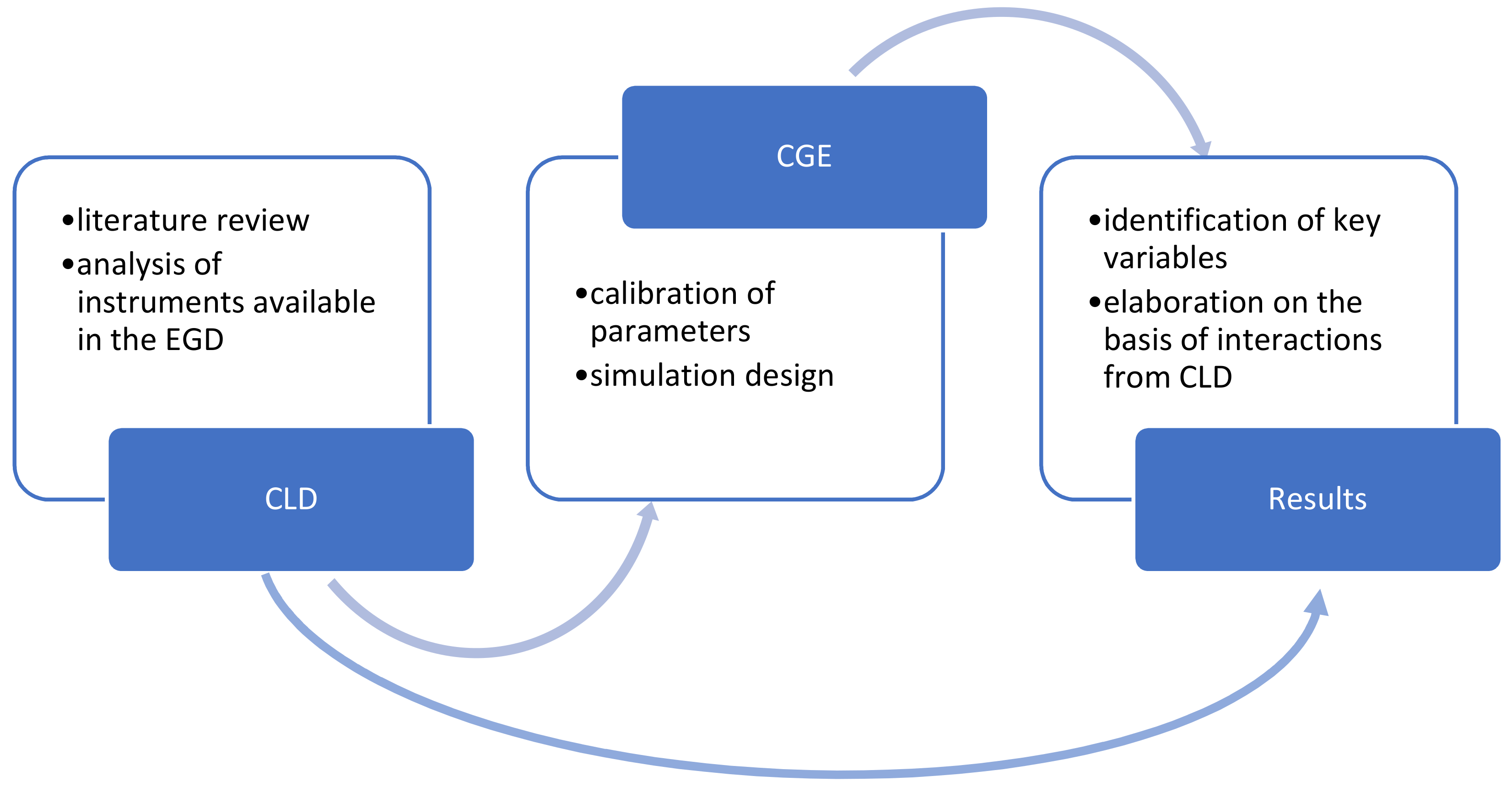
The inclusion of both aspects, agents’ interaction and feedback loops on the one side, and global relations into a market equilibrium approach on the other side, is hard to implement in a single model as different logics and behaviours drive the two elements. On the other hand, a soft-linking approach might help exploit the advantages of both tools by informing each other. In this paper we propose a one-way linkage approach, where the agents’ interaction is defined with a system thinking approach, and the direction of linkages are used to develop a dynamic CGE model and formulate policy scenarios.
In particular, CGE models provide reliable results in a long-term perspective but they are affected by a strong rigidity in modelling assumptions, as for instance fixed technical coefficients, homogeneous agents and no feedback loops that can change behavioural parameters, such as demand elasticity to price and income, substitution elasticity across inputs in the production function, or substitution elasticity in consumer (households) basket expenditure.
All these sources of rigidity might be smoothed by first applying a ST approach to draw a complete picture of the complexity of the dynamic linkages arising from the policy issue under investigation. Then, parameters and coefficients in the CGE model can be updated or modelled as exogenous shocks on the basis of the ST indications, and simulation results are selected and interpreted from the point of view of the evolution of complex systems.
Figure 1 presents a flow diagram for the approach used to develop the research presented in this paper. First, a literature review was performed, considering the overall strategy of the EGD, policy provisions envisaged and expected outcomes. The review of data and historical trends as well as policy ambition and expected impacts resulted in the creation of the CLD. Two versions were created, one focused on system dynamics and one included policy intervention options. The former was used to support simulation designed for the CGE model, while the latter was used to perform policy analysis and support the interpretation of the results of the CGE model. The quantitative analysis includes both the parametrization and calibration of the pre-existing GDynEP model, as well as the creation of scenarios and resulting simulation of the model. Finally, the results of the study are a combination of insights originating from the use of systems thinking (CLD) and quantitative modelling (CGE), where key systems’ variables were identified and numerical results interpreted.

2.1. Systems Thinking

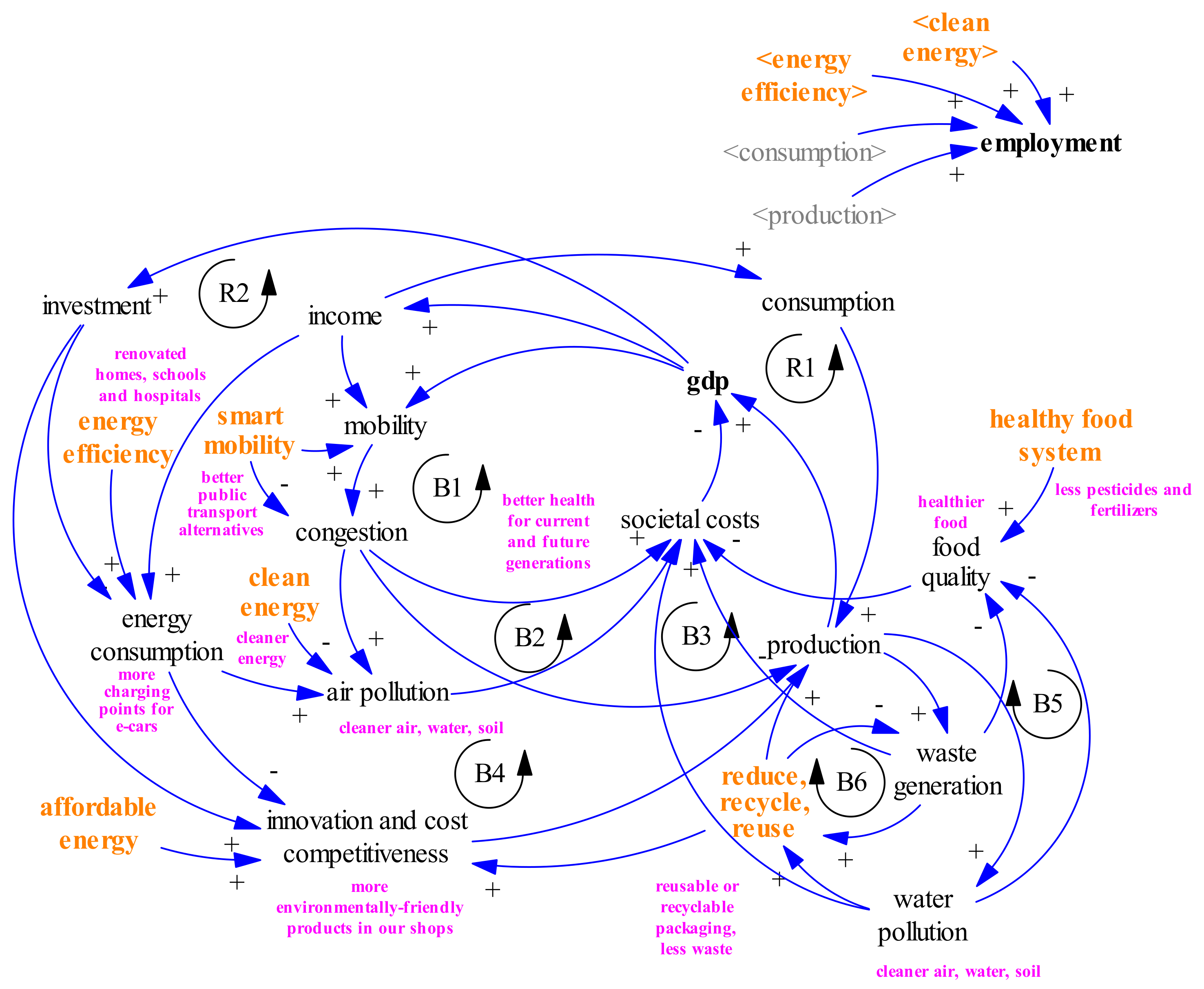
The starting point for the systemic analysis is the review of past drivers of change and the dynamics these have triggered. With an understanding of the known patterns of change that brought us to the need for the introduction of the EGD it will be possible to identify stated entry points for intervention, and their direct, indirect and induced outcomes. The use of ST provides a simplified system map (or causal loop diagram, CLD) to understand how the key variables of our socioeconomic and environmental system are interrelated, and how policy intervention can shift the dynamics experienced historically, leading to a more sustainable future. The CLDs presented in this paper were created with the software Vensim. Figure 2 shows that when GDP increases, a stable trend in the past decades, with only a few exceptions, two main outcomes emerge: (a) consumption increases, leading to higher GDP directly and indirectly via production (reinforcing loop R1), and (b) investment increases, leading to more innovation and cost competitiveness, in turn increasing production and GDP (reinforcing loop R2). It is these reinforcing loops (R) that trigger economic growth, also through employment creation and trade.
On the other hand, economic growth has given rise to various balancing factors (or balancing loops). One of these is the growing need for mobility, resulting in congestion. Congestion increases time spent in traffic and away from work and families (B1), creating societal costs. It also reduces the potential to grow for productivity, production and value added (B3). It further leads to air pollution (B2) resulting from energy use (both for transport, industries and in buildings), which affects labour productivity via health. Finally, the increase in energy use resulting from higher investment and income has led to higher vulnerability to market dynamics, price volatility and extreme weather events impacting the supply of energy (B4), which has negative impacts on production. Production, in turn, leads to the generation of waste, which impacts water pollution and food quality, creating societal costs both in urban and rural areas (B5). These are only a few examples of growing costs to society, those highlighted in the EGD. In addition, these costs are not emerging in the same measure in all countries and regions. As an example, urban areas are being impacted more strongly by air pollution than rural areas.
When considering historical trends, it emerges that the reinforcing loops R1 and R2 have been dominating the dynamics of the system. This is because GDP, consumption and investment have grown over time, as have congestion and societal costs. On the other hand, the reinforcing dynamics have been stronger and have dominated the economy over the balancing ones. In 2009, after the financial crisis of 2008, GDP and investments decreased by 4.3% and 11.7%, respectively, for the EU27+UK. However, between 2015 and 2018 GDP increased by 2–2.5% each year, while investments also grew by 2.3–4.9% during the same period. Moreover, consumption expenditure increased by 9.8% from 2008 to 2018 on the basis of information on national accounts provided by Eurostat [23]. On the other hand, thanks to energy efficiency improvements, little change has emerged for energy consumption and emissions, as well as for waste generation, indicating relative decoupling. Gross inland energy consumption was relatively stable between 1990 and 2017, increasing only by 1.6% according to the national energy balances [24] while greenhouse gas emissions were around 22% lower than 1990 levels as emphasised by the statistics provided by the European Environment Agency (EEA) [25]. According to Eurostat, waste generation, excluding major mineral waste, slightly increased from 779.5 million tonnes in 2004 to 785.0 million tonnes in 2016 [26], thus revealing that deeper investigation on specific environment-related themes might unveil inefficiencies in the sustainability of the development trajectory. Overall, this highlights that the emergence of balancing loops has been countered by energy efficiency, the use of renewable energy, collection, sorting, recycling and reuse of waste. Limiting these balancing factors has allowed GDP to continue growing at 1.5–2.5% in the last decade, but more should be done both to support the economy via reinforcing loops and reducing constraints to growth via balancing loops.
The EGD is designed to use various strategies (in orange in Figure 2) to influence energy, buildings, transport and food production. The expected outcomes (in pink) include cleaner air, water and soils (through interventions on energy efficiency, clean energy, waste reduction, improved agriculture practices), also resulting in better human health, better transport alternatives and access to distributed power generation options (and so better access to more modern and resilient services).
Specifically, energy efficiency, clean energy and affordable energy are designed to reduce energy consumption and air pollution, as well as to stimulate innovation and increase competitiveness. As a result, these interventions strengthen reinforcing loops R1 and R2 via GDP, consumption and investment. At the same time, balancing loops B2, B3 and B4 will become weaker, further stimulating economic growth by reducing societal costs and making production more effective. Investments to realize these opportunities include renovated homes, schools and hospitals (energy efficiency), renewable energy use, installation of charging stations for e-vehicles, and adoption of environment-friendly technologies (clean and affordable energy). Smart mobility via better public transport and non-motorized transport will make B1 and B2 weaker, by reducing congestion, energy use and emissions, leading to lower societal costs (e.g., health costs) and more effective production activities. Outcomes include better health for current and future generations, via cleaner air, water, soil (also in conjunction with waste reduction, recycling and reuse). Waste reduction, recycling and reuse affect primarily B5 and B6, which then indirectly affect R1 and R2. As a result, reducing waste both unlocks opportunities for existing drivers of growth, and stimulates new paths for sustainable growth by stimulating innovation and competitiveness. Healthy food systems are expected to increase food quality by reducing the use of fertilizers and pesticides. This reduces societal costs (B2, B3), increasing labour productivity, lowering public and private costs, resulting in a stimulus taking place through R1 and R2.
Practically, the EGD aims at making balancing factors weaker, so that the economy can continue to grow, but in a more sustainable and resilient way. This results in lower costs for society, higher productivity, and improved well-being.
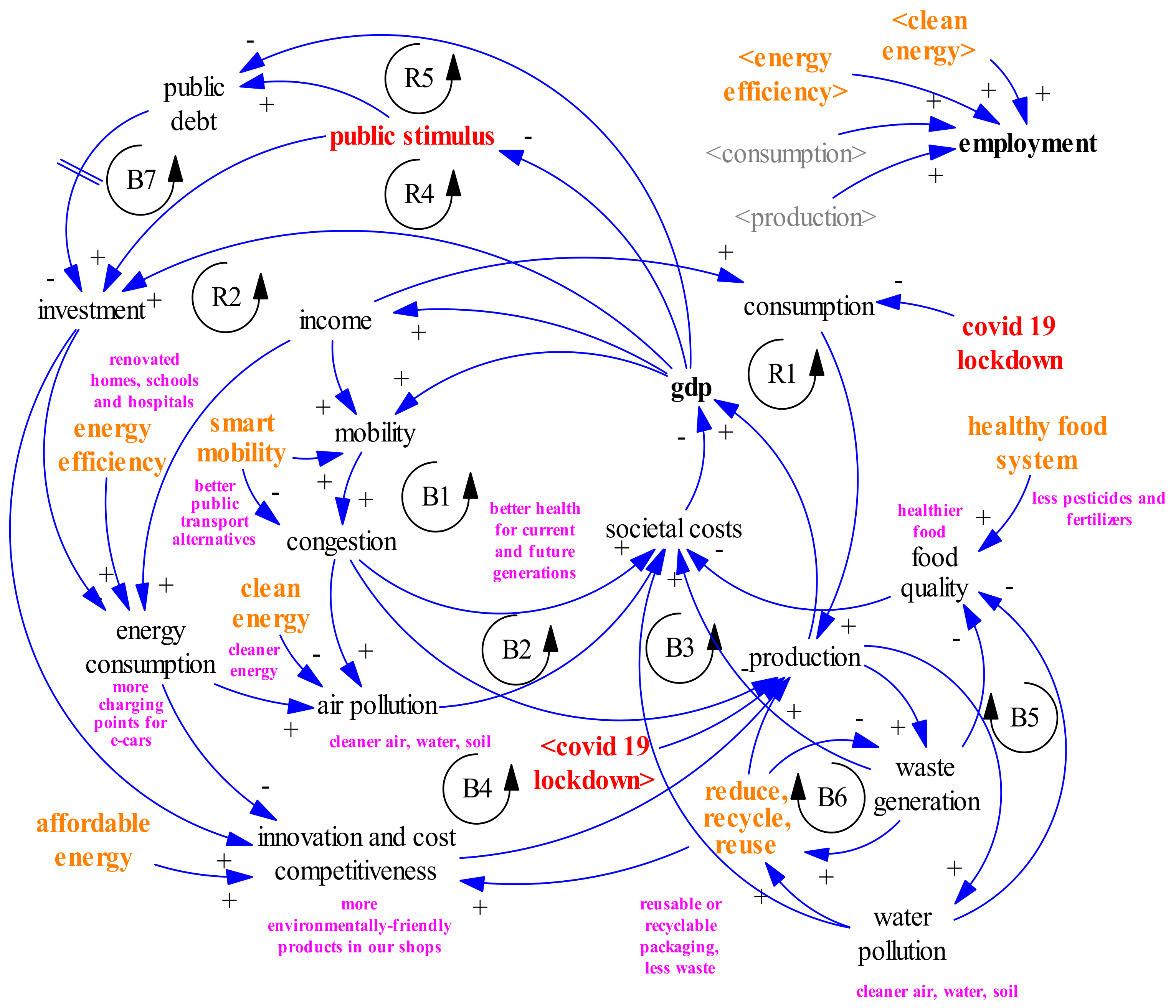
The inclusion of the COVID-19 pandemic crisis in the analysis requires the addition of several variables to the CLD, representing (i) impacts of the outbreak (e.g., consumption) and (ii) response measures (e.g., public stimulus). These additions introduce new dynamics and feedback loops (Figure 3), namely:
  • reduction of GDP via the reduction of production (due to demand and limited labour force availability);
  • reduction of GDP via the reduction of consumption (due to social distancing, avoided travel);
  • reduced economic performance due to the higher cost of doing business and insurance premiums;
  • reduced country performance due to the increase of country risk and public costs (higher country risk leading to higher debt costs, higher public costs related to health and stimulus packages).
These four dynamics affect two existing reinforcing loops (R1 and R2), having a negative impact on GDP via consumption and production, possibly triggering a vicious cycle and hence a recession. The introduction of a public stimulus instead adds reinforcing loops R4 and R5. The former represents the short-term solution implemented by governments, to stimulate investments. The latter represents the expectation that, once the economy starts growing again, it will generate additional growth that allows the reduction of the debt accumulated in the short-term. The dynamics triggered by the increase of debt are represented by the balancing loop B4. Higher debt will reduce the potential for new investments in the future, due to the higher cost of debt servicing and to budget constraints related to financial stability.
It has emerged that COVID-19 has temporarily turned two drivers of growth (R1 and R2) from virtuous to vicious, making them causes of recession rather than growth. This triggers balancing loop B7, which highlights the limited (finite) amount of financial resources available to governments. The expectation is that, if the stimulus is allocated well (R4), after the lockdown ends and the economy recovers, it will kick start production and consumption to levels that will stimulate employment, increase government revenues (R5) and limit the constraints posed by medium and long-term debt (B7).
Concerning environmental performance, the reduction of economic activity reduces energy consumption and air pollution, and hence societal impacts, driven by R2, as well as by B1, B2, B3 and B4. With economic recovery the opposite dynamics return, as described earlier. As a result, little change is expected to these dynamics, unless permanent impacts emerge (e.g., smart working remains common practice with a structural impact on transport modes).

2.2. The GDynEP Model

By focusing on the behavioural aspects related to the energy system, some of the linkages and loops obtained by the ST approach can be simulated into a dynamic CGE model hereafter called GDynEP. The model we develop for this purpose is based on RunDynam software designed for GTAP-type models. The specific GTAP-type version of the model is called GDynEP and all details on the modelling approach are provided in [27,28]. With respect to the previous GDynEP model version, there are some novelties related to the construction of the base year, the emissions data and the regional aggregation.
The base year relies on the GTAP 10 database, meaning that the starting point is the year 2014, with updated values for Leontief input-output matrices for the factor costs of sectors included. The GTAP 10 database is a consistent representation of the world economy for a pre-determined reference year [29].
Together with combustion-based CO2 emissions as in all standard GTAP-E models, the GDynEP also introduces non-CO2 emissions associated with the use of energy commodities in the production and consumption activities. In detail, the new version of GDynEP includes three energy-related data sources.
The GTAP-E 10 database provides carbon dioxide (CO2) emissions data distinguished by fuel and by user for each of the 141 countries/regions and the 65 sectors in the GTAP10 database. GTAP-E data is based on: GTAP 10 and extended energy balances compiled by the International Energy Agency (IEA). A complete description of all features in the GTAP-E database is provided by [30].
The GTAP-Power 10 database is an electricity-detailed extension of the GTAP 10 database including seven base load technologies (nuclear, coal, gas, hydroelectric, oil, wind and other power technologies), and four peak load technologies (gas, oil, hydroelectric, and solar) for 2014 [31]. Moreover, an updated version of the methodology allows output of the electricity and heat generation sector to be split using electricity generation data together with heat generation volumes [32].
The GTAP-NCO2_V10a database is based on the methodology developed by [33] and is integrated in GDynEP with three major non-CO2 groups of gases, CH4, N2O, and fluorinated gases (F-gases), including CF4, HFCs, and SF6. Emissions come from three emissions drivers: consumption (by consumers and firms), endowment use (land and capital), and output. With respect to the emissions associated with consumption by firms and households the original GTAP file has been transformed in order to be compatible with the structure of combustion-based CO2 emissions used in GTAP-Power with 76 sectors. Accordingly, the new emissions database contains the sum of combustion-based CO2 emissions and non-CO2 emissions associated with the use of energy inputs including the chemical sector.
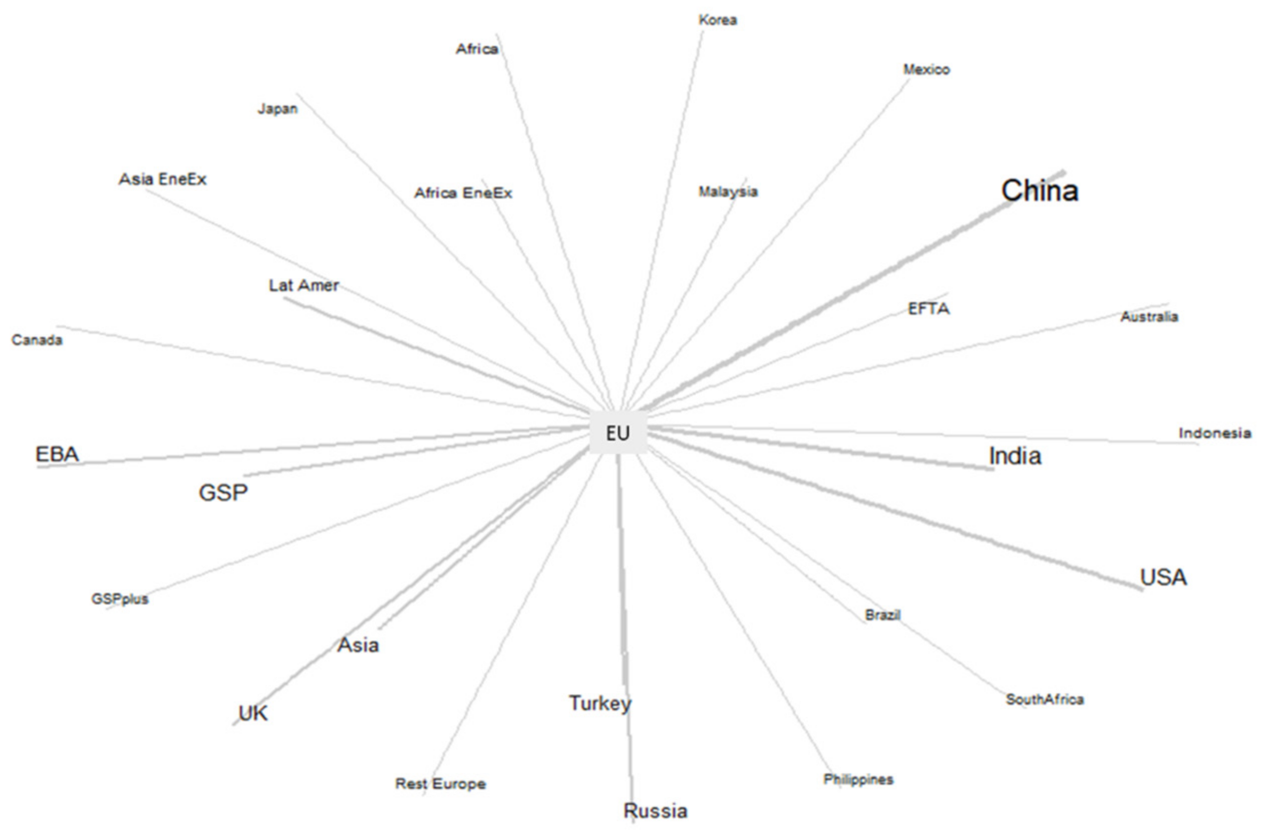
The regional aggregation: takes into account the Brexit process and the United Kingdom is excluded by the EU aggregate, while the sector aggregation is based on the technological content as well as the energy intensity of the production process. Details on aggregation are provided in Appendix A, Table A1, Table A2 and Table A3.
With respect to the time frame, the starting point is 2014, so the first period is 2014–2015, while the following periods are five-year steps up to 2050 with a total of eight periods. Details regarding the software adopted, the aggregation files, the elaboration of shocks are available in the Supplementary Material file.

2.3. Simulation Setup

Scenarios are based on a business as usual reference case (BAU) that is alternatively tested with and without the economic crisis due to COVID-19 pandemic. This helps us better investigate the role played by investments in clean energy technologies (CETs) in contributing also to exiting the crisis. By comparing the GDP growth rate with COVID-19 shock with growth patterns associated with a general economic recovery based on GDP levels, it is possible to highlight the magnitude of investments required to escape from the crisis in a short-term perspective. By adding the financial support to CETs associated with the implementation of the EGD targets, we can emphasize the additional impact played by longer term investments.
The source on which scenarios are based is divided between the current period 2014–2020 and projections for the time span 2025–2050. The different variables on which the baseline and the policy scenarios are based are listed.

2.3.1. Model Calibration to Current Baseline

For what concerns the calibration for the current period 2014–2020, we provide details on the procedure adopted for each variable.
  • Population: for the reference period (2014) data are taken from the GTAP10 database while for updates 2015–2020, data come from Eurostat and World Development Indicators (WDI) from the World Bank;
  • CO2 emissions: for the reference period on combustion-based CO2 emissions (2014) data are taken from GTAP-E while for updates 2015–2020, data come from Eurostat, IEA CO2 emissions highlights and WDI;
  • GDP: for the reference period (2014) data are taken from the GTAP10 database while for updates 2015–2020, data come from Eurostat and WDI;
  • Non-CO2 emissions: for the reference period (2014) data are based on GTAP-NCO2V10a updated with change in 2015–2020 based on Eurostat and IEA energy balances;
  • Labour force: for the reference period (2014) data for skilled and unskilled labour force are calculated as the share of total labour force from CEPII information applied to GTAP population data and for the period 2015–2020 they are also calibrated with ILO information on labour force and CEPII statistics;
  • Production of electricity from renewable sources (RSELE) in the electricity sector: for the reference period (2014) data on RSELE are taken from GTAP Power version 10 and for the period 2015–2020 data comes from growth rates computed on Eurostat and IEA energy balances;
  • Production of electricity from fossil fuels (FFELE): for the reference period (2014) data on FFELE are taken from GTAP Power version 10 and for the period 2015–2020 data come from growth rates computed on Eurostat and IEA energy balances.
For the projections in the time span 2025–2050, the baseline case (called BAU) is computed on the basis of the combination of data from different sources:
  • Data on GDP, population, GHG emissions and production of electricity divided into RSELE and FFELE are based on the reference case used by the JRC model (Keramidas et al., 2020) for all regions in the model setting except for the EU region;
  • data on GDP, population, GHG emissions and production of electricity divided into RSELE and FFELE only for the EU members with country-based information are based on the reference case developed by the European Commission for the PRIMES model [34];
  • Data on labour force divided into skilled and unskilled are based on CEPII projections [35].
The baseline is calibrated with shocks associated with GDP, population, skilled and unskilled labour force and CO2 and non-CO2 emissions that are considered as exogenous and are calibrated with the increase in production and consumption efficiency. This is a requirement for the GTAP modelling exercise because otherwise emissions are not bounded, and they proportionally follow the GDP and population trends without any assumptions on technological improvements that will reduce carbon intensity of economic dynamics.
A further element for building the BAU case is reflected in the energy balances for all regions, and in particular the proportion of renewable and fossil fuel sources in the electricity production process. On the basis of the projections available from the JRC model and the EU reference case for PRIMES, the two electricity sub-domains have been treated as exogenous, thus calibrating the BAU case at the end of 2050 with a share of RSELE on total electricity for the EU compatible with the JRC baseline case. The shocks in BAU are based on the evolution over time of the production of electricity by the two sources expressed in GWh, where the starting point is 2014 according to the value of electricity production provided in the GTAP-Power database in GWh. The calibration has also been compared with the composition of the energy mix on the consumption side with respect to the reference case of the EU models, in order to obtain an overall energy consumption at the EU level compatible with expected values simulated with the help of bottom-up technology scenarios.

2.3.2. Model Calibration for Policy Scenarios—Paris Agreement

For the projections in the time span 2025–2050 related to the policy case, we consider as a starting point the decarbonization process for the EU27 region according to the implementation of the Paris Agreement with an emissions pattern to 2050 compatible with the EU targets associated with the increase in global temperature by a maximum of 1.5 °C with respect to pre-industrial levels. The emissions target designed for the Paris Agreement scenario for the EU is equivalent to the net zero emissions target described in the EGD with the updated target by 2030 of cutting emissions by 55% with respect to 1990 levels. Accordingly, there is a common CO2-eq emissions trend in all policy scenarios for the EU.
Given that the GDynEP model is an economic-energy model without enough technological details to simulate the role played by LULUCF and CCS activities, the final emissions in 2050 account for gross emission levels without the impacts of carbon sinks. This results in an apparent overestimation of emissions with respect to the EU reference scenario that is fully explained by the absence of sinks. Accordingly, while in the EU reference case emissions in 2050 are around 2% of the BAU case, in GDynEP in 2050 emissions are around 9% of the BAU case. The remaining 7% is supposed to be absorbed by carbon sinks to reach the target of net zero emissions by 2050.
In order to obtain the first policy scenario in which the EU will respect the abatement target for the full implementation of the Paris Agreement, resulting in an emission reduction by 2050 of 91% with respect to the BAU case (called EU-PA), a policy instrument based on a Pigouvian carbon tax is adopted. According to the model version in Bassi et al. (2020), by considering the EU as an aggregated region it is worth mentioning that the cost effectiveness criterion is fully respected, since the value at the margin of the carbon tax is perfectly equivalent to a carbon price level if an emission trading system is applied. The only difference between the EU-ETS and the modelling approach we adopt is that in GDyn-EP all sectors are involved in the carbon policy with the same instrument, without differentiated treatment for energy-intensive and non-energy intensive sectors [28]. This assumption allows consideration of carbon tax and carbon price as fully equivalent market-based environmental policy instruments. Accordingly, in the following sections we will consider carbon tax and carbon price as if they are synonymous.
In order to calibrate the model with respect to the emissions trend, we take CO2 emissions as exogenous only for the EU, with a specific trend that is compatible with the PA target. On the contrary, emissions for the rest of the world are left as endogenous, considering a case in which the other regions are not respecting their NDCs under the PA. This is consistent with a notion of unilateral policy, and in a comparative exercise perspective, it is the only way to compute the economic impacts of a specific policy in an ex-ante evaluation with a counter factual benchmark. If, on the other hand, we adopt a multilateral perspective in which all regions implement abatement targets, it is no longer possible to single out the economic impact of the EGD [36].
Together with the calibration of emissions with exogenous shocks, we also control for the energy mix at the EU level, with particular attention to electricity production. More specifically, we consider electricity production, both from fossil fuels and for RES as exogenous, following the production trends available in GECO 1.5 °C policy case. This is a requirement because electricity is a carbon free energy source in a sense that consuming electricity is not associated with CO2 emissions. This leads to an overestimation of electricity consumption in a policy scenario with no control for electricity production. In other words, the model cannot consider for instance technical constraints to substitutability between sources related to competition to inputs (capital and labour mainly), or diffusion obstacles, for example, associated with the absorptive and distribution capacity of the power grid.

2.3.3. Model Calibration for Policy Scenarios—European Green Deal

In order to make an economic assessment of the impacts associated with the EGD, on top of the first policy scenario (EU-PA), based on a simple carbon pricing instrument, we associate an additional instrument based on a revenue recycling mechanism for financing the development, deployment and diffusion of CETs. The recycling mechanism is based on the hypothesis that part of the revenues collected from carbon pricing (CTR) by the government can be reused for sustaining green energy technologies.
In detail, given that GDynEP has a standard production structure where sectors are classified according to the ISIC codes, without a specific sector producing technology, we compute an elasticity parameter with which investment flows in R&D are directly transformed into benefits on the consumption and production side.
We test different shares of CTR to be allocated to finance CETs through an ideal innovation fund that can be compared with real figures available in the estimation provided for the ETS innovation fund by the European Commission. It is worth mentioning that in our model, given that a carbon price (equivalent to an equilibrium carbon tax) is paid by all sectors (as if the ETS has been applied to the whole economy without free allowances), from the one side the higher the abatement target the higher the cost, given by the carbon price, but on the other hand a higher carbon price is associated with a larger CTR and consequently to a higher amount of the innovation fund for CETs.
In GDynEP it is possible to account for the efforts in development and diffusion of two technology options: energy efficiency, both in the production processes and in the households’ consumption patterns; and production of electricity with renewable sources.
In order to quantify the contribution of public support to CETs, we need two parameters related to elasticity of substitution that are required for developing evolutionary scenarios of technological trajectories for clean energy technologies sustained by public support [37]. We compute them on historical data for the last ten years of R&D public investments in the EU for energy efficiency (obtained in all sectors) and renewable sources in electricity with respect to the starting date of GDynEP (2014). In this model we consider two assumptions: (i) energy efficiency uniformly influences productivity across all sectors independently from the specific share of energy used within the input mix, (ii) the diffusion of innovation is not influenced by additional technical barriers different from those already accounted for with the historical estimation.
The model is programmed in order to use R&D investments to increase input augmenting technical change for the use of energy as an input in the consumption (households) and production (firms) function. For a given amount of public budget invested in energy efficiency, the effect consists of a reduction of the energy intensity with respect to the reference case, with a lower cost for saving energy [38].
Concerning renewable sources in electricity generation, by promoting renewable energies by capacity investments (rather than by generation subsidies) the impact of uncertainty for demand conditions and capacity availability is substantially reduced. Accordingly, the elasticity is computed considering the public R&D investment in renewable sources for electricity generation provided by the IEA R&D database and the corresponding increase in installed capacity in renewable electricity in EU countries during the same period (1994–2014 Eurostat energy balance dataset available online). The estimated parameter comprises an output-augmenting technical change, meaning that the R&D efforts have the main effect of reducing the production cost of electricity from renewables with respect to fossil fuel sources. The economic rationale behind this modelling choice is simple: given a certain number of inputs used for producing RES (mainly capital and labour), the investments in RES allow the system to transform the same amount of inputs into a larger amount of output (electricity in this case) [39].
It is worth mentioning that the investments in RES are combined with the exogeneity of RES production in the EU-PA policy case. This means that the amount of RES produced are exogenously determined but the production cost is endogenously driven by the amount of investments directed to technical change from the CTR. Accordingly, the higher the share of CTR invested into the innovation fund, the higher the output augmenting technical change, the lower the unitary production cost. In order to compare model results with the EU energy strategy pillars, in the case of RES it is possible to compare the amount of energy, and in particular of electricity from RES as a share of total consumption of electricity. Given that the production cost is lower, in the EU-GD scenario it is likely to obtain an increase in the share of electricity from RES consumed than in the EU-PA policy scenario.

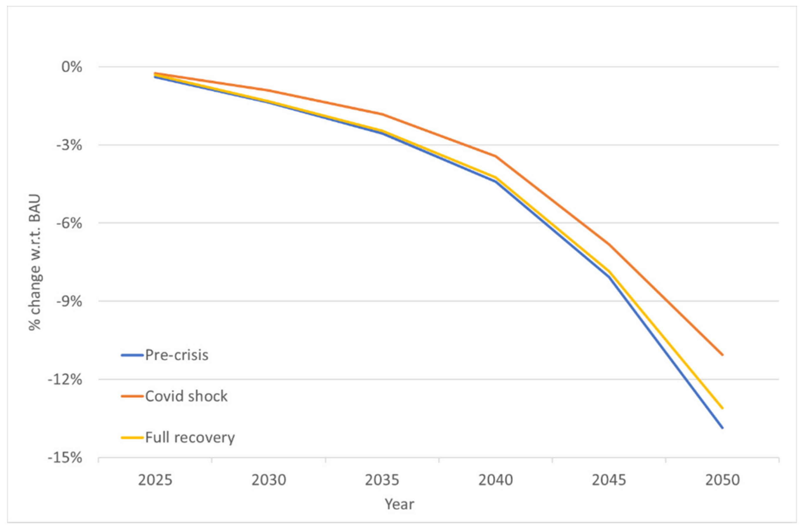
2.3.4. Scenarios Accounting for COVID-19 Crisis

Together with these three scenarios we introduce the economic impact of the crisis due to the COVID-19 pandemic to the BAU case as follows. Starting from the BAU case we implement a policy shock in 2020 with an exogenous reduction of GDP w.r.t. the BAU case with an impact associated with the main regions according to [40] compatible with the IMF and the World Bank estimates at the world level, recently provided by the updated report [41]. The average reduction at the world level is estimated around 6% in 2020 w.r.t. BAU and around 3% w.r.t. the GDP level in 2019.
The economic impacts of COVID-19 are many and varied and growing by the day. Following the outbreak, financial conditions have worsened at an unparalleled speed, weakening economies worldwide. Emerging dynamics include the increased risk of defaults of private companies due to weaker demand, higher volatility in the stock market due to future uncertainty on the profitability of businesses and impacts on the solidity of national finances due to growing expenses and reduced revenues. These impacts depend on both global and local dynamics, with local consumption as well global trade being impacted by the number of infected countries and the duration and severity of epidemiological shocks. The uncertainty of impacts, effectiveness of policy responses, and duration of current challenges leads to consideration and creation of various scenarios for a possible recovery.
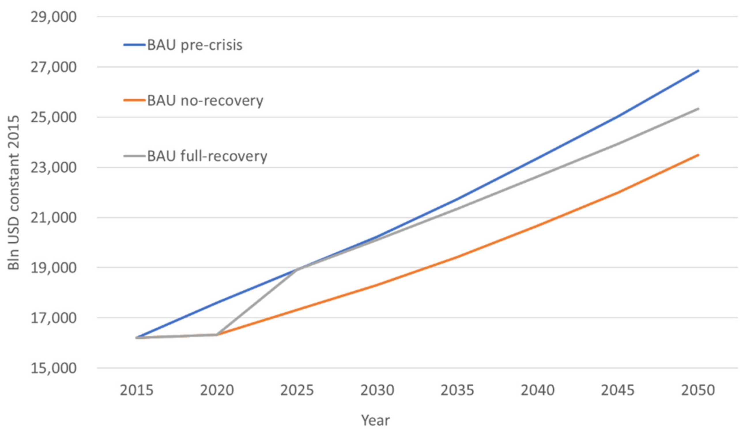
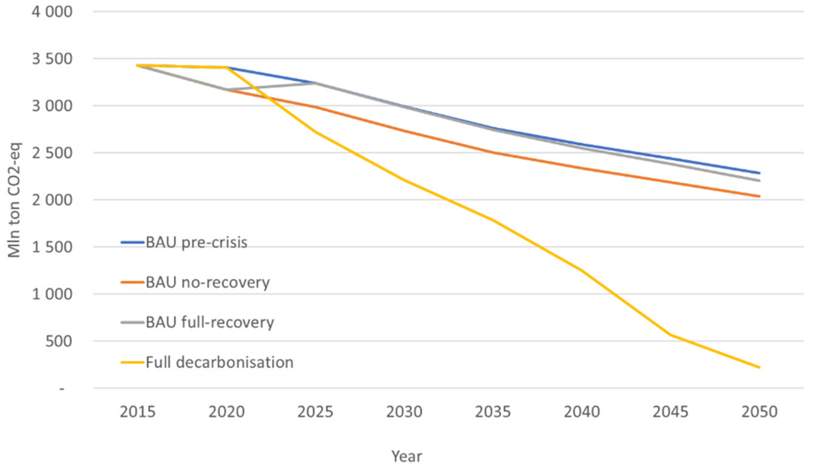
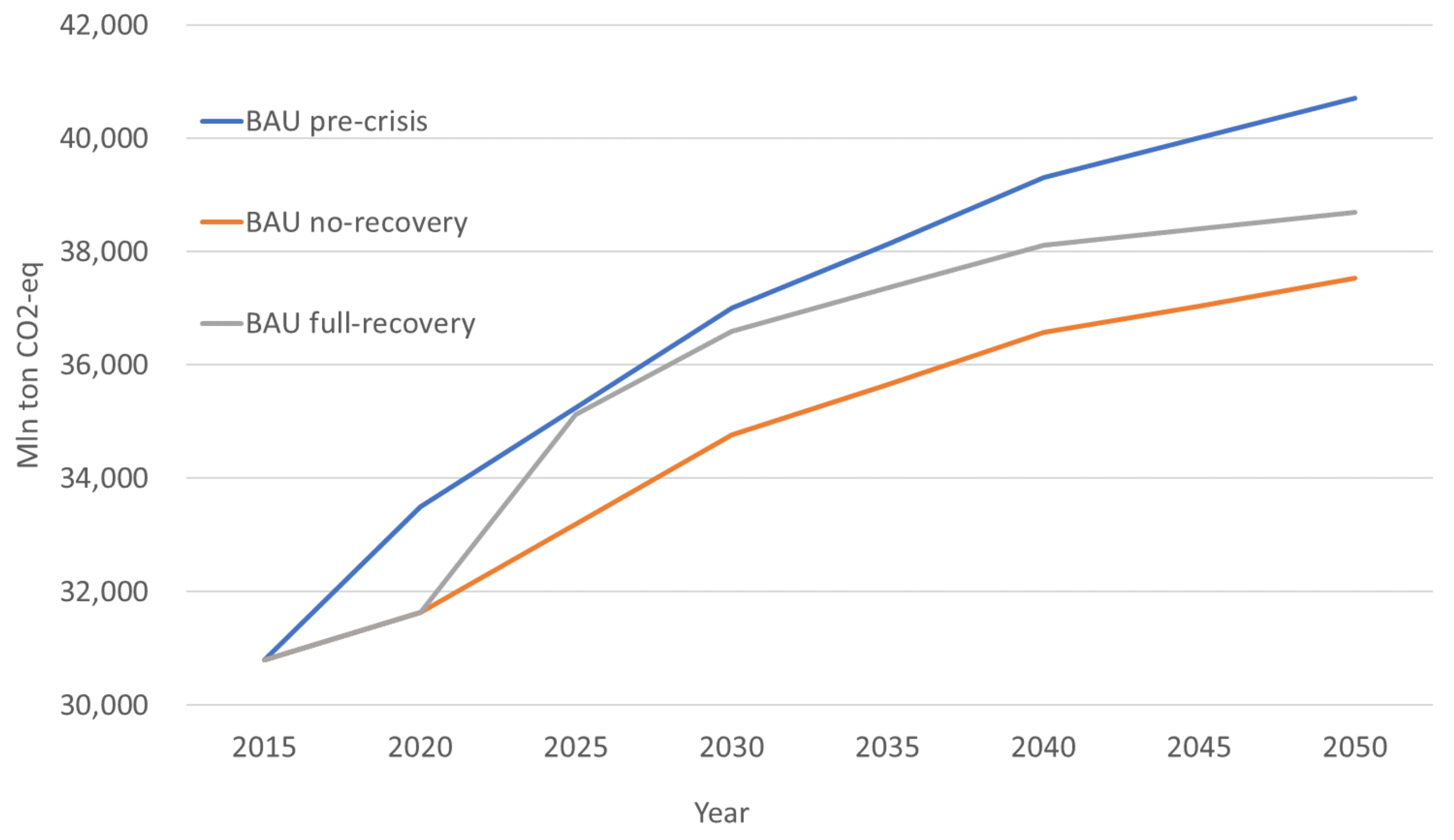
The assumption is that once the shock has been assigned to the 2020 policy scenario, then the GDP is left to be determined endogenously by the model. Accordingly, it is possible to obtain changes in GDP from 2025 according to a path dependence approach related to the dynamic recursive nature of the model. It is worth mentioning that in the case of a COVID-19 shock without any recovery measure, the GDP growth pattern can be lower than in the case of a BAU pre-crisis case because the amount of capital stock for the economic system is dependent on savings produced in the previous period in a system of national account methodology.
The BAU case that accounts for the shock which occurred in 2020 assumes that no additional shocks will occur, but the endogenous solution provides GDP values for the period 2025–2050 that incorporate the negative impacts due to capital stock reduction and a demand decrease that persists over time. This BAU case with the COVID-19 shock with no recovery measures is named BAU no-recovery.
A second scenario is built with an exogenous shock that allows GDP in 2025 to turn back to 2025 original BAU values before the COVID-19, hereafter called BAU full-recovery. This means that the shock is calibrated in order to give impulse to the economic system to completely recover from the negative impacts in the medium-term (5 years). In order to make sure that the amount of resources is compatible with policy feasible solutions, we have computed the endogenous increase in capital formation required to recover from the crisis. As a benchmark, we looked at the resources that the EU is allocating in different forms during 2020 amounting to a recovery package of around €750 billion, that corresponds to around 5% of the EU GDP in 2020 from GDyn-EP without COVID-19. In 2025, according to the full-recovery scenario, the total resources to be invested along a 5-year period required to go back to a GDP pre-COVID-19 amount to around 9.5% of GDP in 2025. Considering that in the years 2021–2025 additional resources could be invested within the Next Generation EU fund according to the recovery plans presented by Member States, together with additional private resources, a total of 9.5% of GDP in the form of capital investments is reasonable. The same mechanism is applied to all regions belonging to the GDyn-EP, with examples of resources invested in other large economies as 4% of GDP in China and 8% in the US.
On the basis of the two additional BAU scenarios that include COVID-19 GDP shock with and without recovery, we are able to compute the new emissions trend for the two BAU cases. Different from the original BAU where emissions are exogenously projected according to bottom-up energy scenarios, in the two BAU cases with COVID-19 emissions are left free to move endogenously, following the GDP shocks in 2020 and in 2025 (only in the case of full-recovery), and the endogenous GDP patterns from 2025 on. Accordingly, together with the GDP, CO2-eq emissions will also be changed with respect to a BAU pre-crisis, and on this new reference case the two policy options associated with the simple carbon pricing and the additional measures planned within the EGD are implemented and evaluated. As a final calibration check, emissions endogenously determined with the BAU no-recovery and BAU full-recovery GDP shocks have been compared with emissions provided by the bottom-up model by the International Energy Agency available in the World Energy Outlook 2020 [42].

3. Results

3.1. Economic Impacts with COVID and Unilateral European Union Carbon Pricing

The BAU case represents a baseline to be used as a benchmark for policy impact evaluation under different scenarios and assumptions. The introduction of the economic shocks associated with the COVID-19 pandemic is represented for the EU in Figure 4 and for the rest of the world (ROW) in Figure 5.
The difference highlighted by the two alternative patterns is explained by the introduction of a generally designed recovery package that is supposed to be implemented over five years, from 2020 to 2024, in order to obtain a full recovery in 2025. After 2025 the GDP pattern is endogenous again and the recursive nature of the dynamic CGE implemented here demonstrates that without a long-term perspective in the design of the implementation of investments under the recovery measures, the positive impulse to GDP is large in the short-term but loses weight in the medium to long term. The reason behind this result is that from 2020 to 2025 a considerable portion of capital stock has been lost, and the resources implemented for a short-term recovery are not sufficient for ensuring a return to the same GDP growth pattern. Practically, reinforcing loops R1 and R2 (see Figure 3) will not be strong as in the BAU scenario in the medium and long term, despite the stimulus offered by R4. Possible reasons, in addition to loss of capital, include the future cost of the recovery package (e.g., cost of financing) and the economic growth pattern being largely aligned with the carbon intensity and the creation of externalities of the BAU scenario.
According to the modelling choice described in Section 2.3.4, together with the GDP pattern that is endogenously modelled from 2025 on, the CO2-eq emissions included in GDynEP are also left free to evolve according to the economic patterns at the regional level and the feedback loop mechanisms automatically activated as shown. As a result, the reduction in economic activities even in the case of a full recovery in 2025 will bring emissions in the BAU case to decrease, both in the case of EU (Figure 6) and ROW (Figure 7).
In Figure 6 we compare emission trends for the EU in the different BAU cases with the projection of the full decarbonisation strategy by 2050. Emissions decline in the decarbonisation scenarios as a result of the implementation of intervention options that reduce energy use and stimulate fuel switching (see Figure 3, specifically, orange variables and feedback loops B2, B3 and B4).
It is worth mentioning that, although in both post-COVID reference scenarios the CO2 level will drop, the emission gap with the mitigation target is still large. The implementation of a unilateral carbon policy by the EU will instigate a reaction at the global level with an increase in emissions level, as a typical carbon leakage effect [25]. This means that the efforts taken by the EU in reducing emission levels that correspond to around 2000 Mt CO2-eq abated in 2050 w.r.t. BAU are partly cancelled out by the increase in emissions by the rest of the world (estimated around 1000 Mt CO2-eq), with a carbon leakage rate (computed as the ratio between the change in emissions of the ROW and the absolute value of emission reduction by the EU) by 2050 that is around 51%. In other words, if the emission reduction by the EU is implemented by adopting a carbon pricing instrument alone, without any additional public support for speeding up the technological transition of the energy sector, the reaction of foreign producers will be to increase their demand for fossil fuels to produce goods and services thanks to their increased competitiveness on external markets with respect to the EU companies. Furthermore, whatever BAU is considered, the achievement of the emissions level respectful of the EU decarbonisation target obtained by a pure carbon price policy without any support to efficiency and innovation has relevant costs for the EU, with a substantial drop in GDP level (Figure 8). This is not surprising, as the final target for the year 2050 is a reduction of 90% in emissions w.r.t. to 2050 emissions in BAU, corresponding to a net zero emission goal for the EU, with a carbon price that is prohibitive in all scenarios without any financial support to CETs.
Competitiveness losses are obviously more evident for energy intensive sectors, as those included in the EU ETS. By looking at the relations with the ROW, changes in emission patterns are disentangled across sectors and computed as the difference in emissions produced by each sector by all other regions forming the ROW with respect to the decrease in EU emissions for the same sectors associated with the implementation of the climate policy. It is worth noting that the chemical, energy and transport sectors are the leading players in the leakage effect (Figure 9). The reaction by foreign countries to the EU climate policy when implemented only with a market-based instrument without support to CETs is to increase the volume of production activities to fill the gap provoked by the reduction in EU output. Indeed, the market-based mechanism brings a substantial competitiveness loss to EU firms, and an increase in comparative advantages with resulting offshoring effects that undermine the benefits from the EU climate policy.
Together with a sector disaggregation of the leakage effect, it is relevant to investigate if and to what extent there are selected trade partners that are involved more than others by this offshoring mechanism. Given the structure of GDynEP, it is not possible to disentangle to what extent the offshoring effect is associated with a delocalization process of EU firms that moved abroad or to an increase in production activities decided at the local level by foreign firms. Accordingly, results must be interpreted as a delocalization of the source of emissions that are embedded into EU imports rather than into EU domestic production, with only a partial reproduction of the mechanisms and linkages related to innovation and competitiveness highlighted with the ST approach (Figure 2 and Figure 3, reinforcing loop R2), which primarily represent the extent to which the adoption of new technology and the reduction of externalities will support innovation and competitiveness in the EU. The quantification of this offshoring mechanism with a bilateral trade dimension is graphically represented in Figure 10.
Putting the EU in the middle of the import network, the dimension of the name of each region and the thickness of the arc connecting the EU with each partner is proportional to the difference between the emissions embedded in bilateral import flows in the policy scenario w.r.t. the reference case. Accordingly, a large share of the offshoring effect in producing emissions abroad to satisfy the EU internal demand for final goods and intermediate inputs is associated with few regions, namely China, India, USA, GSP UK, EBA and Russia, here listed according to their relative relevance, and representing more than 60% of the total emissions embedded into EU imports.

3.2. Economic Impacts with Full Implementation of the EGD

When the unilateral carbon pricing mechanism is complemented by the public support to CETs’ deployment and diffusion, the overall cost of achieving the target is considerably lower and the situation changes. In this simulation we test the impact of an innovation fund mechanism that is financed by 50% of 100% of the pricing mechanisms in the form of carbon tax revenue (CTR) derived from the collection of the Pigouvian tax (remembering that it is equivalent to a carbon price in an ETS covering the whole economy with no free allowances).
The final economic impact measured by GDP pattern under the two CTR share scenarios reveals that GDP level increases with respect to the reference case, and this positive outcome is proportional to the share of resources devoted to financing CETs. When the maximum share is tested, we can notice that the increase in GDP assumes a positive and stable trend resulting in a constant increase in GDP w.r.t. the BAU case (Figure 11).
By considering the reaction in structural composition of the global economy, differences in technologies and emission intensities across regions explain the changes in emissions of ROW as a consequence of international outsourcing or offshoring [43]. Contrary to the case when only a carbon pricing mechanism is implemented, when the full EGD is tested, the leakage effect is reversed and becomes slightly negative when the 100% share of CTR is simulated (Figure 12). A possible explanation of this result is associated with trade-induced positive knowledge spillover effects, in the form of a direct transfer of carbon-neutral technologies to foreign producers or an improvement in the environmental quality of EU goods exported in the global market and used as intermediate inputs [44].

4. Discussion

The first key result we obtain from interpreting the CGE outcome with a ST approach is that the efficiency gains determined by the full implementation of the EGD allow the transformation of EU climate policy into a development opportunity, with a complete decarbonisation target achieved with noticeable economic benefits, revealing that a sustainable energy transition is not only feasible but also profitable. This results from the synergies created in simultaneously strengthening reinforcing loops (e.g., R1 and R2) and making balancing loops weaker (e.g., B1 through B6) in Figure 2 and Figure 3.
Indeed, the unitary abatement cost of one ton of CO2-eq by 2050 is more than halved when the carbon tax revenue is recycled for CETs improvement. In addition, it is worth mentioning that a higher share of revenue devoted to CETs is a key element for cost competitiveness for the EU as the unitary carbon price is inversely correlated with the share of CTR recycled.
The second result we stress refers to the contribution of this complex multi-method approach in interpreting potential trade-offs into instruments’ interaction. According to the CGE outcomes, given that the amount of resources invested in clean energy technologies via the innovation fund is endogenously determined by the abatement target, that in turn influences the carbon price level, the reduction in carbon price obtained with a higher revenue share also results in a relative reduction in the proportionality of the amount of the innovation fund. Consequently, the higher the share of carbon tax revenue the higher the innovation fund but with a decreasing proportionality. This is a clear example of the multiple linkages that should be considered under a complexity approach, as the final value of the investment fund is simultaneously affected by a positive impact related to the increase in the share of revenue recycled and by a negative impact associated with the reduction in carbon price. The lower the carbon price the smaller is the revenue collected from carbon pricing, and consequently the amount of resources to be invested in the innovation fund. Such a trade-off might be well explained by the feedback loops activated by joint effects played by the carbon pricing instrument and the public support to innovation deployment related to the revenues collected by the government.
The third noteworthy result refers to the additional elements provided by a general equilibrium approach to the interlinkages that can be detected at the domestic level. The positive effects associated with the loops activated by the EGD within the EU countries are followed by additional benefits at the global level thanks to positive knowledge externalities creating a race to the top effect in trade relationships and the adoption of cleaner technologies also in extra-EU countries.
This analysis and the results obtained are far from perfect. Nevertheless, the emergence of synergies from the use of multi-methods is evident. The qualitative analysis of key drivers of change, with a dynamic approach, can support the creation of a quantitative assessment, as well as improve the interpretation of the results obtained. Identifying the best entry points for intervention, so as to maximize efficiency and value for money for policy interventions is critical, especially when new investments are implemented to emerge out of an economic crisis.
The CLDs, being qualitative and not constrained by data availability, allow for the creation of a shared understanding of the dynamics of the system analysed. In our work, we use CLDs as a blueprint for model and scenario formulation as well as for the interpretation of results. First, CLDs highlight how policy outcomes may materialize in the form of synergies or side effects; second, being more comprehensive than a CGE model, CLDs extend the quantitative analysis with dimensions and dynamics that cannot be quantified (e.g., either due to the characteristics and limitations of the CGE, or any other quantitative model, or due to the qualitative nature of certain dynamics, possibly related to behavioural choices and emerging patterns of behaviour). As a result, both qualitative and quantitative approaches provide much needed information to policymakers, reaching beyond the typical limitations of each approach taken alone (i.e., quantification is required, but it is often narrowly focused, or not as all-encompassing as reality is).
This multi-method approach allows formulation of a key policy implication that has been scarcely addressed by previous quantitative studies. The adoption of multiple market-based instruments, typically in the form of demand and supply-side policies (represented in this case by the carbon pricing and the support to R&D activities, respectively), even if they are well balanced [45], might generate inefficiencies in the exploitation of marginal gains in technological opportunities. A better knowledge of the multiple qualitative linkages occurring in society between stakeholders might inform the policy making process in activating corrective measures that might maximise the returns to investments in clean energy technologies.
Despite the limitations of a such multi-method framework, mainly related to the rigidity of the CGE structure that cannot follow all linkages provided by the CLD, we see great potential of such an approach to be applied to other scenario analyses.
Indeed, the methodological improvement provided by such a soft-linking exercise is well represented by the calibration and interpretation of changes in CGE results when including the macroeconomic effects provoked by an external shock, as in the case of COVID-19. The additional effects and feedback loops obtained with a pandemic-corrected CLD are key inputs for both setting the scenario in the CGE model, but more importantly for immediately highlighting those quantitative results that are mainly affected by this shock.
Such an exercise could be adapted to further shocks, such as large changes in energy prices due to unpredictable events (e.g., due to a conflict occurring in large fossil fuels suppliers or to a disruptive innovation discovery radically shifting the technological trajectory) that could be hardly modelled in a precise way with a CGE model alone.
As a result, although this work is at an early development stage, it constitutes the basis that can stimulate further efforts in developing complex, systems models.
As an example, the soft-linkage framework can help designing additional fiscal policies that can help turn decreasing marginal returns to scale of knowledge creation in clean technologies into increasing gains thanks to the maximisation of positive loops across stakeholders. Such effects can be used to inform the CGE framework by introducing assumptions that allow positive externalities to dynamically influence returns to scale of innovation, such as those related to knowledge co-creation in a typical smart specialisation policy design.
It is our hope that the proposed approach will be used to better design quantitative analysis and better interpret its results, with broader boundaries. The soft-linking of ST with quantitative models can be applied at different levels and for several assessments, from macroeconomic (as presented in this study) to sectoral (e.g., energy planning) to specific investment and policy decisions (e.g., asset-level analysis for project finance decisions).

5. Conclusions

This work is a first attempt to analyse, with a systemic approach, the effectiveness of policy interventions required to achieve different but interconnected targets by combining a qualitative and a quantitative method. The mixed-method utilised, primarily serving as a framework for knowledge integration, allows for a better calibration of scenario design and consequently provides a more complete interpretation framework of policy outcomes. This holistic approach effectively supports policy formulation and evaluation, especially in light of the growing complexity brought about by COVID-19 and related policy responses. It does so by reducing the drawbacks encountered when using sectoral models with limited boundaries (because these normally focus on a single theme or sectoral dimension and do not allow to create an analysis with the breadth of the EGD), as well as by reducing the complexity of several hard-linked models (where several assumptions have to be made for the simulation of different models that use different equation solving methods and treatment of time). As a result, we find that the approach proposed of soft-linking ST and an existing CGE model both leverages existing knowledge and models, as well as improving the analysis carried out with such models, making the analysis better aligned with the complexity of our socio-economic systems.

Supplementary Materials

The following are available online at https://www.mdpi.com/article/10.3390/su13116303/s1.

Author Contributions

Conceptualization, A.M.B. and V.C.; methodology, A.M.B. and V.C.; software, A.M.B., V.C. and E.P.; validation, A.M.B., V.C. and E.P.; formal analysis, V.C. and E.P.; investigation, A.M.B., V.C. and E.P.; resources, A.M.B. and V.C.; data curation, E.P.; writing—original draft preparation, A.M.B., V.C. and E.P.; writing—review and editing, A.M.B., V.C. and E.P.; visualization, A.M.B., V.C. and E.P.; funding acquisition, A.M.B. and V.C. All authors have read and agreed to the published version of the manuscript.

Funding

This research was funded by the European Environmental Agency (EEA), project EA/IEA/18/001-ETC/WMGE Action Plan 1 Work Programme 2021 (task 5.2.1), by the Italian Ministry of University and Research (MIUR), Scientific Research Program of National Relevance PRIN2017 project “Innovation for global challenges in a connected world: the role of local resources and socio-economic conditions”, and by the European Commission, DG Trade Chief Economist Tender TRADE 2019/G2/G10 “Trade and climate change: an energy-economic modelling approach”.

Institutional Review Board Statement

Not applicable.

Informed Consent Statement

Not applicable.

Data Availability Statement

Data for CGE simulation are not available since they are covered by copyright and can be used only GTAP subscribers.

Acknowledgments

Comments, discussions and suggestions from several persons enriched the current development of the research. Among them, we are particularly indebted with by Alessandro Antimiani, Marco Guzzetti, Massimiliano Mazzanti, Lars Nilsson, Stefan Speck and Roberto Zoboli for their continuous stimuli and support.

Conflicts of Interest

The authors declare no conflict of interest.

Appendix A

Table A1. GDynEP aggregation of endowments.
No.Model CodeDescription
1LandLand
2SkLabSkilled labour force
3UnSkLabUnskilled labour force
4CapitalCapital
5NatResNatural resources
Table A2. GDynEP aggregation of economic sectors.
No.Model CodeDescriptionSector Code
1riceRicepdr, pcr
2cerCereal grainswht, gro
3o_primOther primaryosd, pfb, ocr, wol
4vegVegetable and fruitv_f
5livLivestockctl, oap
6r_meatRumin meatcmt
7o_meatOther meatomt
8fishFisheryfsh
9daiDairyrmk, mil
10bev_tBeverages and tobaccob_t
11foodProcessed foodvol, ofd
12sugSugarc_b, sgr
13texTextiletex, wap, lea
14papPaper and publishingppp
15woodWoodfrs, lum
16chemChemicalchm, rpp
17pharPharmaceuticsbph
18minMineralnmm, oxt
19motMotor vehiclesmvh
20tr_eqTransport equipmentotn
21electElectronics and electronic eqele, eeq
22metalMetal productfmp
23machMachineryome
24ferFerrous metali_s, nfm
25o_manOther manufacturingomf
26coalCoalcoa
27oilOil crudeoil
28gasNatural gas and LNGgas, gdt
29ely_fElectricity from fossil fuelsNuclearBL, CoalBL, GasBL, OilBL, OilP, GasP
30ely_rwElectricity from renewablesHydroBL, HydroP, OtherBL, SolarP, WindBL
31oil_pOil productsp_c
32r_transpRoad and railway transportotp
33a_transpAir transportatp
34w_transpWater transportwtp
35serv1Service privateTnD, ofi, ins, rsa, obs, whs, cmn, trd, cns, afs
36serv2Service publicros, osg, hht, edu, wtr, dwe
Table A3. GDynEP aggregation of regions.
No.Model CodeDescriptionRegion Code
1AFDC Africa developing countriescmr, zwe, bwa, nam
2AFEX Africa energy exportersegy, xnf
3AFNorth Africa Northmar, tun
4AS1 Rest of East Asiaaze, geo, isr, jor, xws
5AS2 Asian countries (rest of)twn, xea, brn, khm, sgp, tha
6ASEXMiddleEast &Asian energy exp.kaz, bhr, irn, kwt, omn, qat, sau, are
7Australia Australiaaus
8Brazil Brazilbra
9Canada Canadacan
10ColPeru Colombia and Perucol, per
11China China plus Hong Kongchn, hkg
12EBA Everything but arms countrieslao, xse, bgd, npl, xsa, ben, bfa, gin, sen, tgo, xwf, xac, eth, mdg, mwi, moz, rwa, tza, uga, zmb, xec, xsc
13EFTA EFTA countriesxna, che, nor, xef
14EU27 European Union membersaut, bel, bgr, hrv, cyp, cze, dnk, est, fin, fra, deu, grc, hun, irl, ita, lva, l tu, lux, mlt, nld, pol, prt, rou, svk, svn, esp, swe
15GSP GSP countriesxoc, vnm, tjk, xsu, civ, gha, nga, xcf, ken, mus
16GSPplus GSP plus countriesmng, pak, lka, bol, kgz, arm
17India Indiaind
18Indonesia Indonesiaidn
19Japan Japanjpn
20Korea South Koreakor
21Malaysia Malaysia mys
22Mexico Mexicomex
23NewZealand New Zealandnzl
24Philippines Philippinesphl
25RestAndean Rest of Andean countrieschl, ecu, ven, xtw
26RestEurope Rest of Europealb, blr, ukr, xee, xer
27RestLatAmer Rest of Latin Americaxsm, cri, gtm, hnd, nic, pan, slv, xca, dom, jam, pri, tto, xcb
28RestMercosur Rest of Mercosurarg, pry, ury
29Russia Russian Federationrus
30SouthAfrica South Africazaf
31Turkey Turkeytur
32UK UKgbr
33USA USAusa

References

  1. European Commission (EC). Communication from the Commission to the European Parliament, the European Council, the Council, the European Economic and Social Committee and the Committee of the Regions ‘The European Green Deal’; European Commission: Brussels, Belgium, 2019. [Google Scholar]
  2. European Environment Agency (EEA). The European Environment—State and Outlook 2020: Knowledge for Transition to a Sustainable Europe; European Environment Agency: København, Denmark, 2019. [Google Scholar]
  3. Bergh, J.V.D.; Castro, J.; Drews, S.; Exadaktylos, F.; Foramitti, J.; Klein, F.; Konc, T.; Savin, I. Designing an effective climate-policy mix: Accounting for instrument synergy. Clim. Policy 2021. [Google Scholar] [CrossRef]
  4. Tinbergen, J. On the Theory of Economic Policy; North Holland Publishing Company: Amsterdam, The Netherlands, 1952. [Google Scholar]
  5. Tinbergen, J. Economic Policy: Principles and Design; North Holland Publishing Company: Amsterdam, The Netherlands, 1956. [Google Scholar]
  6. Bennear, L.S.; Stavins, R.N. Second-best theory and the use of multiple policy instruments. Environ. Resour. Econ. 2007, 37, 111–129. [Google Scholar] [CrossRef]
  7. Bouma, J.A.; Verbraak, M.; Dietz, F.; Brouwer, R. Policy mix: Mess or merit? J. Environ. Econ. Policy 2019, 8, 32–47. [Google Scholar] [CrossRef]
  8. Geels, F.W.; Sovacool, B.K.; Schwanen, T.; Sorrell, S. Sociotechnical transitions for deep decarbonization. Science 2017, 357, 1242–1244. [Google Scholar] [CrossRef]
  9. Rogge, K.S.; Reichardt, K. Policy mixes for sustainability transitions: An extended concept and framework for analysis. Res. Policy 2016, 45, 1620–1635. [Google Scholar] [CrossRef]
  10. Bassi, A.M. Moving towards integrated policy formulation and evaluation: The Green Economy Model (GEM). Environ. Clim. Technol. 2015, 16, 5–19. [Google Scholar] [CrossRef] [Green Version]
  11. United Nations Environment Programme. The Energy Transition as a Key Driver of the COVID-19 Economic Recovery in Panama; United Nations Environment Programme: Nairobi, Kenya, 2020. [Google Scholar]
  12. ESPON. CIRCTER—Circular Economy and Territorial Consequences; ESPON EGTC: Luxembourg, 2019. [Google Scholar]
  13. Bassi, A.M.; Perera, O.; Wuennenberg, L.; Pallaske, G. Lake Dal in Srinagar, India: Application of the Sustainable Asset Valuation (SAVi) Methodology for the Analysis of Conservation Options; International Institute for Sustainable Development with support of the MAVA Foundation, EMSD and GIZ: Geneva, Switzerland, 2018. [Google Scholar]
  14. Bassi, A.M.; Pallaske, G.; Stanley, M. An Application of the Sustainable Asset Valuation (SAVi) Methodology to Pelly’s Lake and Stephenfield Reservoir, Manitoba, Canada; IISD: Geneva, Switzerland, 2019. [Google Scholar]
  15. Freire-Gonzalez, J. Environmental taxation and the double dividend hypothesis in CGE modelling literature: A critical review. J. Policy Model. 2018, 40, 194–223. [Google Scholar] [CrossRef]
  16. Freire-González, J. Energy taxation policies can counteract the rebound effect: Analysis within a general equilibrium framework. Energy Effic. 2019, 13, 69–78. [Google Scholar] [CrossRef]
  17. Delarue, E.; Bergh, K.V.D. Carbon mitigation in the electric power sector under cap-and-trade and renewables policies. Energy Policy 2016, 92, 34–44. [Google Scholar] [CrossRef]
  18. Antimiani, A.; Costantini, V.; Martini, C.; Salvatici, L.; Tommasino, C. Assessing alternative solutions to carbon leakage. Energy Econ. 2013, 36, 299–311. [Google Scholar] [CrossRef]
  19. Cairney, P. Complexity Theory in Political Science and Public Policy. Political Stud. Rev. 2012, 10, 346–358. [Google Scholar] [CrossRef]
  20. Delzeit, R.; Beach, R.; Bibas, R.; Britz, W.; Chateau, J.; Freund, F.; Lefevre, J.; Schuenemann, F.; Sulser, T.; Valin, H.; et al. Linking Global CGE models with Sectoral Models to Generate Baseline Scenarios: Approaches, Challenges, and Opportunities. J. Glob. Econ. Anal. 2020, 5, 162–195. [Google Scholar] [CrossRef]
  21. Pavičević, M.; Mangipinto, A.; Nijs, W.; Lombardi, F.; Kavvadias, K.; Navarro, J.P.J.; Colombo, E.; Quoilin, S. The potential of sector coupling in future European energy systems: Soft linking between the Dispa-SET and JRC-EU-TIMES models. Appl. Energy 2020, 267, 115100. [Google Scholar] [CrossRef]
  22. Krook-Riekkola, A.; Berg, C.; Ahlgren, E.O.; Söderholm, P. Challenges in top-down and bottom-up soft-linking: Lessons from linking a Swedish energy system model with a CGE model. Energy 2017, 141, 803–817. [Google Scholar] [CrossRef]
  23. Eurostat. National Accounts and GDP. 2019. Available online: https://ec.europa.eu/eurostat/statistics-explained/index.php/National_accounts_and_GDP#Investment (accessed on 1 March 2021).
  24. Eurostat. Energy Statistics—An Overview. 2019. Available online: https://ec.europa.eu/eurostat/statistics-explained/index.php/Energy_statistics_-_an_overview#Primary_energy_production (accessed on 1 March 2021).
  25. European Environment Agency EEA. Total Greenhouse Gas Emission Trends and Projections in Europe. European Environmental Agency. 2019. Available online: https://www.eea.europa.eu/data-and-maps/indicators/greenhouse-gas-emission-trends-6/assessment-3#:~:text=In%202017%2C%20the%20EU’s%20greenhouse,2%20%25%20from%202017%20to%202018 (accessed on 1 March 2021).
  26. Eurostat. Waste Statistics. 2019. Available online: https://ec.europa.eu/eurostat/statistics-explained/pdfscache/1183.pdf (accessed on 1 March 2021).
  27. Bassi, A.M.; Costantini, V.; Sforna, G. Systemic Modelling Tools to Assess the Green Economy Transition; Eionet Report; ETC/WMGE: Mol, Belgium, 2020. [Google Scholar]
  28. Corradini, M.; Costantini, V.; Markandya, A.; Paglialunga, E.; Sforna, G. A dynamic assessment of instrument interaction and timing alternatives in the EU low-carbon policy mix design. Energy Policy 2018, 120, 73–84. [Google Scholar] [CrossRef]
  29. Aguiar, A.; Chepeliev, M.; Corong, E.L.; McDougall, R.; Van Der Mensbrugghe, D. The GTAP Data Base: Version 10. J. Glob. Econ. Anal. 2019, 4, 1–27. [Google Scholar] [CrossRef] [Green Version]
  30. McDougall, R.; Golub, A. GTAP-E: A Revised Energy-Environmental Version of the GTAP Model. In GTAP Research Memorandum No. 15; Global Trade Analysis Project (GTAP), Purdue University: West Lafayette, Indiana, USA, 2009. [Google Scholar]
  31. Peters, J.C. GTAP-E-Power: An Electricity-detailed Economy-wide Model. J. Glob. Econ. Anal. 2016, 1, 156–187. [Google Scholar] [CrossRef] [Green Version]
  32. Chepeliev, M. GTAP-Power 10 Data Base: A Technical Note. In GTAP Research Memorandum No. 31; Global Trade Analysis Project (GTAP), Purdue University: West Lafayette, Indiana, USA, 2020. [Google Scholar]
  33. Irfanoglu, Z.; van der Mensbrugghe, D. Non-CO2 Documentation V9; Global Trade Analysis Project (GTAP), Purdue University: West Lafayette, Indiana, USA, 2016. [Google Scholar]
  34. European Commission. EU Reference Scenario 2016; European Commission: Brussels, Belgium, 2016. [Google Scholar]
  35. Fouré, J.; Bénassy-Quéré, A.; Fontagné, L. Modelling the world economy at the 2050 horizon. Econ. Transit. 2013, 21, 617–654. [Google Scholar] [CrossRef] [Green Version]
  36. Antimiani, A.; Costantini, V.; Kuik, O.; Paglialunga, E. Mitigation of adverse effects on competitiveness and leakage of unilateral EU climate policy: An assessment of policy instruments. Ecol. Econ. 2016, 128, 246–259. [Google Scholar] [CrossRef]
  37. Bointner, R.; Pezzutto, S.; Sparber, W. Scenarios of public energy research and development expenditures: Financing energy innovation in Europe. Wiley Interdiscip. Rev. Energy Environ. 2016, 5, 470–488. [Google Scholar] [CrossRef]
  38. De Negri, J.F.; Pezzutto, S.; Gantioler, S.; Moser, D.; Sparber, W. A Comprehensive Analysis of Public and Private Funding for Photovoltaics Research and Development in the European Union, Norway, and Turkey. Energies 2020, 13, 2743. [Google Scholar] [CrossRef]
  39. Bointner, R.; Pezzutto, S.; Grilli, G.; Sparber, W. Financing Innovations for the Renewable Energy Transition in Europe. Energies 2016, 9, 990. [Google Scholar] [CrossRef] [Green Version]
  40. McKibbin, W.; Fernando, R. The Global Macroeconomic Impacts of COVID-19: Seven Scenarios. CAMA Working Paper No. 19/2020. 2020. Available online: https://ssrn.com/abstract=3547729 (accessed on 1 March 2021).
  41. IMF. World Economic Outlook, January 2021; International Monetary Fund: Washington, DC, USA, 2021. [Google Scholar]
  42. IEA. World Energy Outlook 2020; International Energy Agency: Paris, Italy, 2020. [Google Scholar]
  43. Hertwich, E.G. Carbon fueling complex global value chains tripled in the period 1995–2012. Energy Econ. 2020, 86, 104651. [Google Scholar] [CrossRef] [Green Version]
  44. Marin, G.; Zanfei, A. Does host market regulation induce cross-border environmental innovation? World Econ. 2019, 42, 2089–2119. [Google Scholar] [CrossRef]
  45. Costantini, V.; Crespi, F.; Palma, A. Characterizing the policy mix and its impact on eco-innovation: A patent analysis of energy-efficient technologies. Res. Policy 2017, 46, 799–819. [Google Scholar] [CrossRef]
Figure 1. Soft-linking diagram procedure.
Sustainability 13 06303 g001
Figure 2. A simplified representation of the dynamics triggered by the European Green Deal (EGD). Legend: All key areas of intervention are covered in the causal loop diagram: energy, buildings, industry, mobility (https://ec.europa.eu/commission/presscorner/detail/en/fs_19_6714, accessed on 1 March 2021); Pink: EU Green Deal benefits for future generations (https://ec.europa.eu/commission/presscorner/detail/en/fs_19_6717, accessed on 1 March 2021); Orange: all key intervention options (areas) (https://eur-lex.europa.eu/legal-content/EN/TXT/HTML/?uri=CELEX:52019DC0640&from=EN, accessed on 1 March 2021).
Sustainability 13 06303 g002
Figure 3. A representation of the dynamics triggered by the European Green Deal (EGD) including COVID-19 pandemic.
Sustainability 13 06303 g003
Figure 4. Gross domestic product (GDP) pattern in EU27 in reference cases (own elaboration on GDynEP results).
Sustainability 13 06303 g004
Figure 5. Gross domestic product (GDP) pattern in rest of the world (ROW) in reference cases (own elaboration on GDynEP results).
Sustainability 13 06303 g005
Figure 6. CO2 emissions pattern in EU27 in reference cases (own elaboration on GDynEP results).
Sustainability 13 06303 g006
Figure 7. CO2 emissions pattern in rest of the world (ROW) in reference cases (own elaboration on GDynEP results).
Sustainability 13 06303 g007
Figure 8. Gross domestic product (GDP) change in EU w.r.t. baseline with carbon pricing alone (own elaboration on GDynEP results).
Sustainability 13 06303 g008
Figure 9. Sector carbon leakage rate with EU carbon pricing policy (own elaboration on GDynEP results).
Sustainability 13 06303 g009
Figure 10. Difference in emissions embedded in bilateral EU imports by 2050 w.r.t. baseline (own elaboration on GDynEP results).
Sustainability 13 06303 g010
Figure 11. Difference in emissions embedded in bilateral EU imports by 2050 w.r.t. baseline (own elaboration on GDynEP results).
Sustainability 13 06303 g011
Figure 12. Carbon leakage rate under different shares of carbon tax revenue (CTR) financing clean energy technologies (CETs) (own elaboration on GDynEP results).
Sustainability 13 06303 g012
Publisher’s Note: MDPI stays neutral with regard to jurisdictional claims in published maps and institutional affiliations.

