Article

An Improved Case-Based Reasoning Model for Simulating Urban Growth

1
College of Geographical Science, Harbin Normal University, Harbin 150025, China
2
College of Mining Engineering, Heilongjiang University of Science and Technology, Harbin 150022, China
*
Author to whom correspondence should be addressed.
Sustainability 2021, 13(11), 6146; https://doi.org/10.3390/su13116146
Submission received: 20 April 2021 / Revised: 12 May 2021 / Accepted: 27 May 2021 / Published: 29 May 2021

Abstract

:
Developing urban growth models enables a better understanding and planning of sustainable urban areas. Case-based reasoning (CBR), in which historical experience is used to solve problems, can be applied to the simulation of complex dynamic systems. However, when applying CBR to urban growth simulation, problems such as inaccurate case description, a single retrieval method, and the lack of a time control mechanism limit its application accuracy. In order to tackle these barriers, this study proposes a CBR model for simulating urban growth. This model includes three parts: (1) the case expression mode containing the “initial state-geographical feature-result” is proposed to adapt the case expression to the urban growth process; (2) in order to improve the reliability of the results, we propose a strategy to introduce the “retrieval quantity” parameter and retrieve multiple similar cases; and (3) a time factor control method based on demand constraints is proposed to improve the power of time control in the algorithm. Finally, the city of Jixi was used as the study area for simulation, and when the “retrieval quantity” is 10, the simulation accuracy reaches 97.02%, kappa is 85.51, and figure of merit (FoM) is 0.1699. The results showed that the proposed method could accurately analyze urban growth.

1. Introduction

Since the start of the 21st century, urbanization, which is an important feature of global change, has gradually become the main process through which human beings change the natural environment and climate [1,2,3]. As urbanization has rapidly progressed, the phenomenon of global urban growth has become normalized; this is especially true in developing countries, where urban growth has become a direct spatial reflection of urbanization [4]. Studies have shown that urban growth leads to environmental changes and impacts ecological service systems. These impacts include reductions in arable land (from global to local), air pollution, biodiversity loss, and climate change [5,6,7]. The sustainable development of urban areas has been seriously threatened.
Studying the characteristics of the urban development process can help to provide reasonable urban growth control or planning policies [8]. Related studies have focused on spatial–temporal change detection [9], driving mechanism analysis [10], macro-ecological and environmental effects analysis [11,12], process modeling construction [13,14], and so on. Among these studies, the spatiotemporal simulation of geographical processes is relatively basic, but it can simulate the continuous evolution process of cities in time and space, according to the internal physical processes and dynamic mechanisms of urban growth. Many scholars have used a variety of prediction methods to model land expansion in different cities, including cellular automata (CA) [15,16], the Flus model [17], the multi-agent system [18,19], the CLUE-S model [20,21], and the system dynamics model [22]. However, the complex urban pattern evolution mechanism makes it difficult to extract relevant knowledge. This makes these models difficult to interpret and reduces their reliability. Therefore, it is necessary to adopt new research methods to break through the existing bottlenecks.
Case-based reasoning (CBR) is a vital reasoning method in the domain of artificial intelligence; it can achieve quantitative analysis and phenomena prediction by relying on historical data, without the need to understand the development mechanism’s conditions [23,24]. In fact, CBR can even achieve quantitative analysis and prediction without needing to scrutinize the mechanism, this makes CBR particularly useful for geography processing, where there is a driving mechanism. Thus, CBR can effectively break through the bottleneck of knowledge acquisition present in traditional models, and therefore improve the reliability of geographic process simulations. It has great potential to solve geoscience problems [25]. Therefore, research into simulating the urban growth process using CBR has great theoretical significance for enriching its methodology and expanding theoretical research. CBR was initial aimed at diagnosing problems, ordering judgments, and generating strategies [26]; however, as knowledge of CBR has expanded, it has become more widely used. In the field of geographic information systems (GIS), CBR has been applied to environmental monitoring [27,28], risk identification [29,30], cartography [31,32,33], and so on. These studies have integrated CBR evaluation and prediction based on GIS spatial data processes and analysis, promoting the development of CBR in GIS research.
Few studies have examined the spatial patterns or evolution processes of geographical phenomena using CBR. Among them, only one has proposed a CBR model for simulating land use changes [23]. This model describes land patches as cases; changes in unknown patches can be inferred by retrieving known changes of similar patches, thus realizing land use change simulations based on CBR. However, this model struggles to directly describe how the process of urban growth leads to observed changes. Furthermore, the single retrieval result leads to a low level of reliability regarding inferences, and the lack of a time control factor in the fuzzy inference cycle makes it difficult to determine the simulation occurrence when simulating urban growth. The present study therefore improves the CBR model regarding the simulation of land use changes and constructs an expanded model for simulating urban growth. This improved CBR model features three main aspects: (1) based on the raster being regarded as the case expression structure, a case expression mode containing “initial state-geographical feature-result” is proposed to adapt the case expression to the process of urban growth; (2) a retrieval strategy is proposed to classify cases according to their “initial state,” and to calculate their similarity according to their “geographical features,” which improves the reliability of the retrieval results; and (3) a time factor control method is developed, based on demand constraints, to improve the power of time control in the algorithm. This model is the first to realize urban growth simulation based on CBR. To evaluate the performance of the model, in this study, the proposed model was applied to simulate the pattern of the municipal district of Jixi in 2015. The results show that this model can effectively simulate the processes of dynamic spatiotemporal change of cities.

2. Materials and Methods

2.1. Study Area

The research area of this paper was the municipal district of Jixi (Figure 1). Jixi, a city in the southeast of Heilongjiang province, is located in the middle latitude zone (130°24′24–133°56′30 E, 44°51′12–46°36′55″ N). The district’s east and southeast borders lie across the sea from Russia, and its border line has a total length of 641 km. Its west and south borders are adjacent to Mudanjiang and its north border is adjacent to Qitaihe. Jixi is rich in minerals and is an important energy and resource security core area in China. Furthermore, its land is fertile and has rich arable resources; the region thus makes important contributions to ensuring China’s food security. Jixi’s complex urban structure is a composite area of coal and grain, and its urban growth rule is not obvious. It is therefore difficult to extract an ideal set of urban land evolution rules. Taking Jixi as the research area therefore provided a robust test of the validity of the model proposed in this paper.

2.2. Data Sources and Processing

The land use classification data of Jixi from 2005, 2010, and 2015 were selected for use in the study. The land types classified include cultivated land, woodland, grassland, water area, urban land, and unused land. According to the relevant literature [34,35], driving indicators that affect urban growth include DEM (digital elevation model) and various distance indicators. These types of indicators and treatment methods are shown in Table 1. The resolution size of all data were 30 m × 30 m and the data processing software used was ArcGIS 10.2.

2.3. The Model

At present, the basic idea of CBR applying to land use change simulation is as follows [33]. Take the land patch as a case unit to arrive at the land type change result in the new case; an old case can be retrieved from the known case base for the new case. When an old case that is most similar to the new case is retrieved, the results of the old case are applied to the new case. On this basis, this paper suggests the following basic idea for applying CBR to urban growth simulation. Taking the land raster unit as the case, the case in the new period can retrieve the most similar cases in the old period, and subsequently the land evolution type of the old case is taken as the urbanization result of the new case. By improving the existing CBR model of land use change [23], this study constructs a CBR model for simulating urban growth using the three aspects of case expression, case retrieval, and case constraint to solve the problems of inaccurate case expression, single case retrieval basis, and lack of time control.

2.3.1. Case Expression and Collection

The case is the basic unit and essence of CBR [36]. A case’s expression structure and mode determine how CBR works.
(1)
Case Expression Structure
The traditional CBR model of land use change takes the patch as the case unit. However, this has a complex expression structure and is not conducive to describing the dynamic urban system. A spatial discrete raster is a regular grid structure; its expression is simple, intuitive, and follows obvious rules. Raster data can generate global changes through local changes in a geographical environment; they represent the most commonly used data source structure in urban growth simulation research. In this study, the case was expressed in the raster structure as it can be highly unified with the spatial discrete raster data in form. This meant that the case expression structure could be adapted to urban growth research.
(2)
Case Expression Mode
The expression mode of the land use change CBR case is “problem-geographic environment-result” [33], which cannot directly describe the case based on grid structure. Furthermore, there are multi-type results of land use change simulation that differ from the Boolean results of urban growth simulation. In view of the above problems, it is necessary to redefine the connotation of the expression mode of urban growth cases. This study therefore presents new modes: “initial state”, “geographic features”, and “result.” The meanings of each component are as follows:
“Initial state” describes the land use type at the beginning of the case. Each case has only one state at a certain time;
“Geographic features” include a set of spatial data indices that affect urban growth. The indicators are the key features that influence the urbanization process (the transformation to urban land) of a case by describing the geographical environment at the beginning of the case change;
“Result” describes the urbanization outcome of the case at the end of the change. It indicates whether or not the case transformed into urban land.
According to the above descriptions, the urban growth case expression mode is as follows:
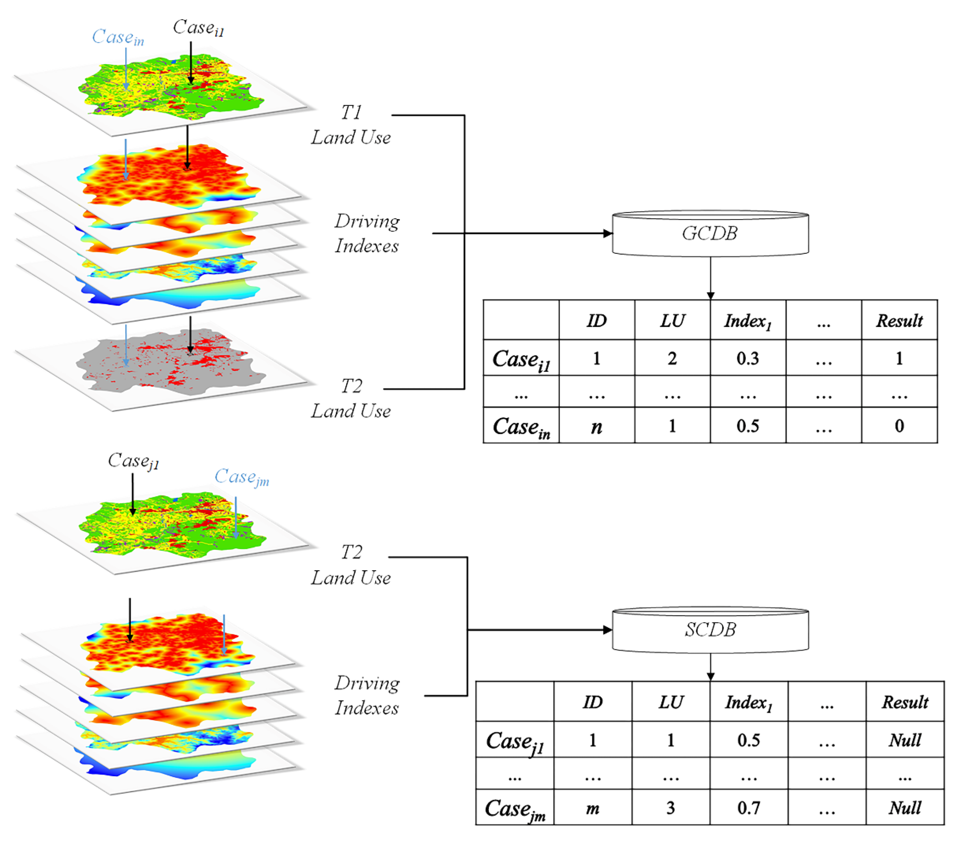
Case i = { L U i ,   I n d e x 1 i ,   I n d e x 2 i ,   ,   I n d e x n i ,   R e s u l t i }
where i is the case number, LUi is the “initial state” of case i, Resulti is the “result,” which is a Boolean variable with an urbanization result of “1” and a non-urbanization result of “0”. Index1i, Index2i, …, Indexni represent the multidimensional “geographical features” index of case i, with a total number of n. Taking a case describing the change process of a land raster from 2005 to 2010 as an example, the “initial state” (LU) is the land use type of the case in 2005, the “geographical features” (Indexn) is geographical feature index of the case in 2005, and the “result” is the urban growth result of the case in 2010.
(3)
Case Collection
In order to study changes in urban growth in different periods, the land use change data of at least two or more periods should be used as the data source when collecting cases. According to their different uses, urban growth cases can be divided into geographical cases and simulated cases, as shown in Figure 2. As they express historical changes in urban growth processes, geographical cases should be constructed based on historical experience, and their “result” should be the basis of the model’s reasoning. Regarding a case being simulated with an unknown “result”, the simulated case should be constructed with known base period data. The simulated case database (SCDB) and the geographical case database (GCDB) are constructed by collecting simulated and geographical cases in a geographical space, respectively.

2.3.2. Case Retrieval

The simulated cases can be matched with the most similar geographical cases through case retrieval; the land use change results can then be obtained. Case retrieval plays a key role in the CBR model and the quality of the retrieval strategy directly affects the efficiency and quality of CBR. [37] The nearest neighbor method is the most commonly used retrieval method in GIS. In order to effectively integrate this method with the CBR model of urban growth, this study first proposes a basic strategy of urban growth case retrieval based on the CBR retrieval mechanism. It then develops an improved comprehensive retrieval strategy.
(1)
Basic Case Retrieval Strategy
The similarity between the two cases can be determined by the similarity of their “geographical features”. It can be concluded that the closer the “geographical characteristics” of the two cases, the higher the similarity between the two cases will be. In addition, considering the effect of the land use type (initial state) of the case on the result, this study proposes a retrieval strategy that classifies cases according to their “initial state”. It then carries out similarity calculations according to their “geographical features”. The detailed retrieval process is as follows.
Firstly, the case base is divided into n sub-case bases according to the “initial state” (“n” is the number of land use types). The GCDB and SCDB with the same “initial state” are classified into the same group, and case retrieval is performed within the same group only. For example, a simulated case with an “initial state” of arable land only needs to be retrieved from geographical cases with an “initial state” of arable land.
Secondly, for each simulated case, all of the geographical cases in the same group are retrieved, based on the “geographical features”, and the nearest neighbor method is used to calculate the similarity coefficient between the cases. The following equation describes this similarity:
S I M l ( P ,   Q i ) = k = 1 n ω k 2 ( p k q k , i ) 2
where l represents the initial land use type of the case, P is the simulated case, Qi is the ith geographical case, SIMl (P, Qi) is the similarity coefficient between the simulated and geographical cases under the land use type l, k is the driving index (geographical features) number, pk is the k of the simulated case, qk,i is the k of the geographical case, wk is the weight assigned to k, and n is the index quantity. The smaller the coefficient value calculated by this method, the higher the similarity between the cases.
Finally, each simulated case selects the most similar geographical case with the minimum similarity coefficient. The “result” of the geographical case is then determined to be the “result” of the simulated case. The following equation describes this process:
R e s u l t j   = R e s u l t i ,   w h e n   S I M j i = S I M m i n
where Resultj represents the result of simulated case j, Resultj represents the result of geographical case i, and SIMji represents the similarity coefficient between cases i and j.
To further illustrate the case retrieval process, Figure 3 introduces an example in detail. Here, a simulated case with an “initial state” of n retrieves all geographical cases with an “initial state” of n. The similarity coefficients (SIMj1, SIMj2 …) are then calculated. If the minimum value (SIMmin) is SIMj2, the “result” of the simulated case j will be inferred to be the “result” of geographical case No. 2.
(2)
Comprehensive Case Retrieval Strategy
Although the nearest neighbor method can retrieve the most similar geographical case, it cannot comprehensively analyze the historical experience. Therefore, the inferred results obtained using the nearest neighbor method are unreliable. To address this, this study improved the basic retrieval strategy and developed a comprehensive one based on multiple geographical cases.
This paper proposes to consider the combined effect of geographical cases with the “results” of 1 and 0. When the role of the urbanization geographical case is stronger (the similarity between the simulated case and the geographical case with a “result” of 1 is higher than that with a “result” of 0), the simulated case will be transformed into urbanization; otherwise, no transformation will occur.
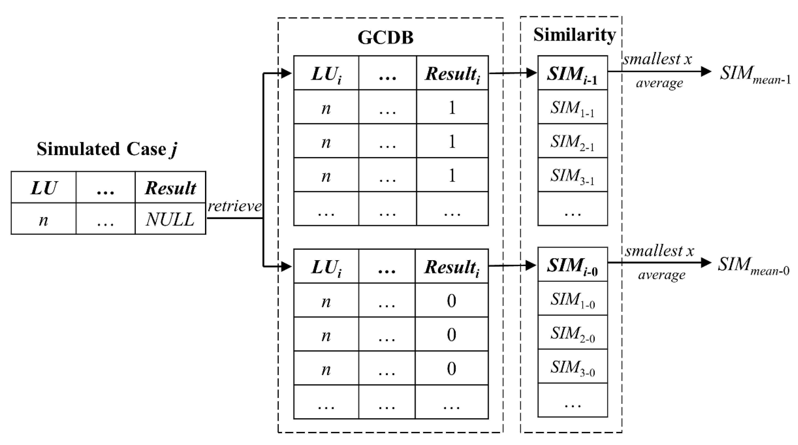
On this basis, we can use the basic retrieval strategy to retrieve geographical cases with “results” of 1 and 0 that are most similar to the simulated case, respectively. By comparing the similarities of the two kinds of case retrieval, the simulated case is determined to be transformed into the “result” of a more similar case. However, when this method is used for simulation, the basis for determining the case result is insubstantial. Therefore, this paper proposes to retrieve multiple geographical cases with two “results” and compare their averaged similarities to determine the “result” of the simulated cases. The retrieval process for simulation case j was as follows (Figure 4):
Firstly, Equation (2) was used to calculate SIMi between the simulated case and each geographical case in the same group.
Secondly, according to the “result” type of the geographical case, SIMi was further classified and represented by SIMi−1 and SIMi−0.
Thirdly, the retrieval quantity, x, was established, and the minimum x values for SIMi−1 and SIMi−0 were taken as the reasoning basis.
Finally, the mean values of the similarity coefficients were calculated as the basis of inference. They were recorded as SIMmean−1 and SIMmean−0, and the result of simulated case j can be inferred according to the following equation:
R e s u l t j = {   1 ,   S I M m e a n - 1     S I M m e a n - 0 0 ,   S I M m e a n - 1   <   S I M m e a n - 0

2.3.3. Case Constraint

Although the results of all simulated cases can be inferred through the above process, the timing of the results of the cases cannot be determined due to a lack of time factor control. This study proposes using the quantity of urban growth over a period of time (quantity demand, QD) to constrain the simulation results. This introduces a time factor in an indirect way to solve the above problems. The specific method is shown in Figure 5: it sorts the average similarity coefficient (SIMmean−1) of all simulated cases with a “result” of “1” from small to large. The top cases are prioritized to be transformed into urban land, and the number of transformations is determined by QD. If the number of simulated cases with a “result” of “1” cannot meet the demand, the remaining simulation cases will be sorted according to SIMmean−1, and a certain number of additional cases will be transformed into urban land until they can meet the needs of urban growth.

2.4. Parameters Preparation and Implementation of Model

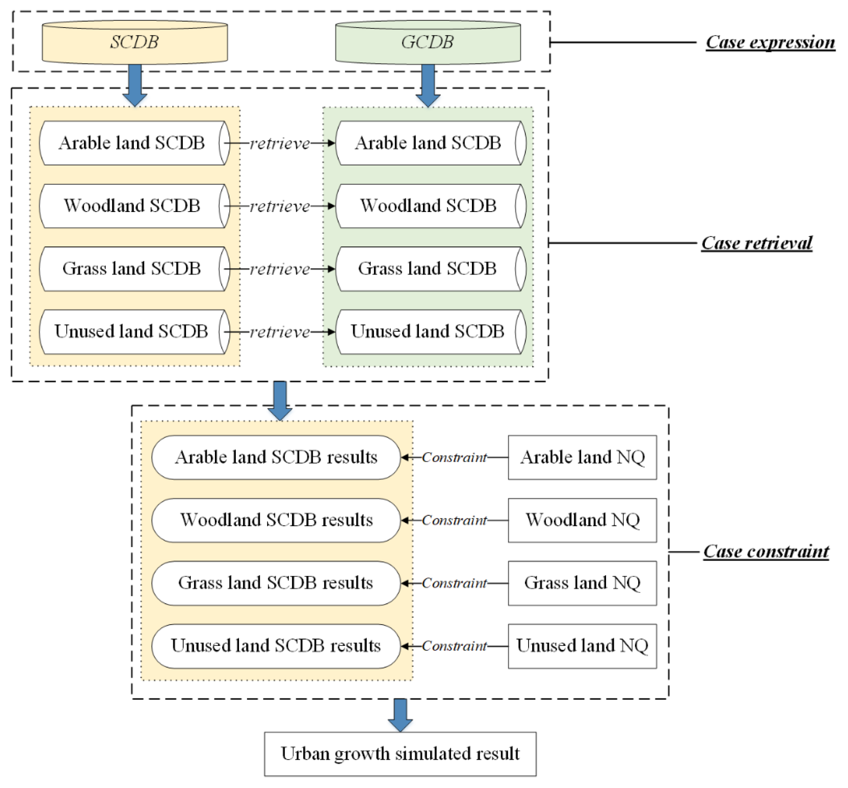
When combined with the case expression, case retrieval, and case constraint processes, a CBR simulation model for urban growth can be constructed (Figure 6). Firstly, the model expresses the simulated and geographical cases of urban growth and constructs SCDB and GCDB, respectively. Secondly, the comprehensive retrieval strategy is adopted to retrieve each simulated case in SCDB and all geographical cases in GCDB in the same group, and the preliminary simulation results are obtained by determining the retrieval results. Finally, through further constraint of the case, the transformation of the cases is further controlled by constraints, and the final simulation results are obtained. This study introduces the implementation process of the model in detail through an experimental approach.

2.4.1. The Implementation of Case Expression

The purpose of this experiment is as follows: the urban growth of Jixi in 2015 was simulated based on land use data from 2005 and 2010. According to this objective, the description periods of the geographical and simulated cases were 2005–2010 and 2010–2015, respectively. According to the urban growth CBR model’s case mode (see Section 2.3.1), the geographical and simulated cases were respectively expressed as follows:
Geographical   c a s e i = { L U 2005 - i ,   D E M ,   D c e n t e r 1 ,   D c e n t e r 2 ,   D e d g e ,   D m i n i n g ,   D w a t e r ,   D r a i l w a y ,   D r o a d ,   R e s u l t 2010 - i }  
Simulated   c a s e j = { L U 2010 - j ,   D E M ,   D c e n t e r 1 ,   D c e n t e r 2 ,   D e d g e ,   D m i n i n g ,   D w a t e r ,   D r a i l w a y ,   D r o a d ,   R e s u l t 2015 - j }
where LU2005−i and LU2010−j separately represent the “initial state”, which are the land use types of each case in 2005 and 2010; DEM, Dcenter1, Dcenter2, Dedge, Dmining, Dwater, Drailway, and Droad represent the various indices, and the year of indices are same as the “initial state”; Result2010−i and Result2015−j separately represent the urban growth “result” in 2010 and 2015.
As the GCDB needs to be classified according to the “initial state” and water areas are not considered to be transformable into urban land, this experiment constructed a GCDB that included four groups: “arable land GCDB”, “woodland GCDB”, “grass land GCDB”, and “unused land GCDB”. To ensure the reliability of model simulation and the efficiency of operation, the experiment randomly and uniformly collected 15,000 cases with “results” of 1 and 0 from each GCDB group. When the total number of cases was insufficient, all the cases of this type were collected. The collection quantity of each group’s GCDB is shown in Table 2.
As with the groupings of the GCDB, the SCDB also included four types: “arable land SCDB”, “woodland SCDB”, “grass land SCDB”, and “unused land SCDB”. The construction of each SCDB required the collection of all simulated cases of each type. The numbers of simulated cases collected in each group are shown in Table 3.

2.4.2. The Implementation of Case Retrieval

According to the process presented in Section 2.3.2, Equation (2) was used for retrieval, and a certain number of geographical cases (including cases with “results” of 0 and 1) were retrieved from each simulated case (the “retrieval quantity” parameter x). The mean SIMmean−1 and SIMmean−0 of the similarity coefficients were calculated, respectively, and the preliminary results of the simulation cases were obtained according to Equation (4).
During the retrieval process, the weight of each index was calculated using the entropy weight method [38]. As case retrieval was only conducted between the simulated and geographical cases in the same group, a set of weights needed to be obtained for each group of each case base (Table 4). In the retrieval process, x determines the reasoning basis. In order to select the appropriate x value, x was set as two, five, ten, 20, 50, and 100 to analyze the influence of x on the simulation accuracy. The implementation of the retrieval process was developed using Python 2.7.

2.4.3. The Implementation of Case Constraint

In this experiment, the QD (Table 5) for urban growth during 2010–2015 was obtained through the spatial overlay analysis function in ArcGIS 10.2. After ranking the simulated cases according to the averaged similarity coefficient (SIMmean−1) from small to large, the number of urbanization cases was controlled to be the same as the QD (in Section 2.3.3), and urban growth was simulated for Jixi in 2015.

3. Results and Discussion

3.1. Evaluation of Authenticity of Simulation Result

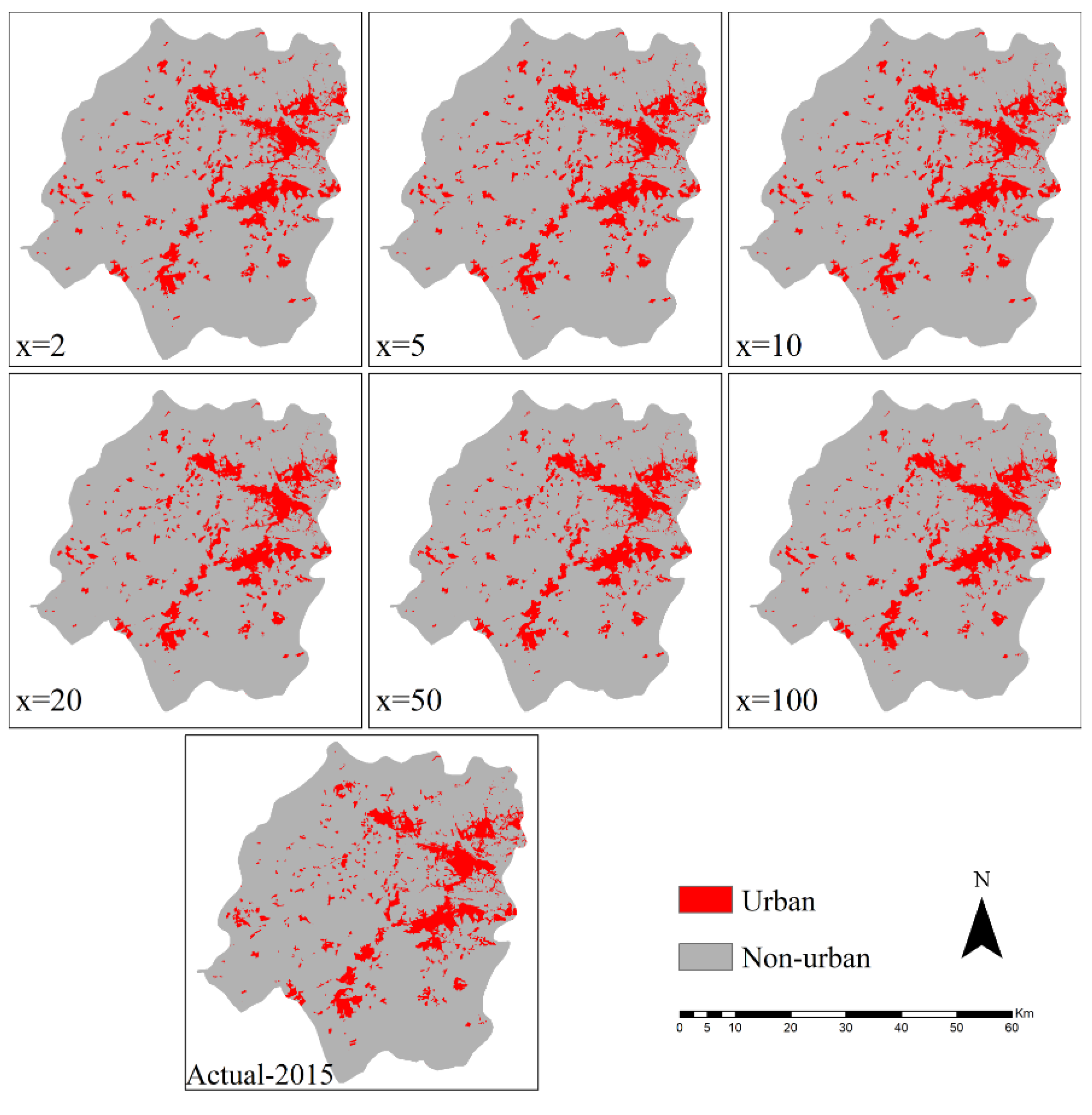
The simplest verification method for the model’s accuracy is to intuitively compare the simulation results with actual results [34]. Through visual inspection, the simulated urban pattern of Jixi in 2015 was compared with the actual urban pattern (Figure 7); the simulated pattern was basically similar to the real pattern. A confusion matrix of the concordance between the simulated and actual situations was then obtained to conduct quantitative analysis (Table 6), and the results show that the simulation accuracy reaches more than 96% and the kappa coefficient is also above 85% (Table 7). In addition, since figure of merit (FoM) is better than kappa with regards to the accuracy of evaluating the simulation changes [39], this paper adopts FoM to further evaluate the accuracy. The calculation formula is:
F o M = B / ( A + B + D )  
In this formula, A is the area of non-urban land that is transformed into urban land in the actual scenario, but not in the simulation scenario. B is the area of non-urban land transformed into urban land in both scenarios (the correctly transformed area). D is the area of non-urban land that is not transformed into urban land in the actual scenario, but is in the simulation scenario.
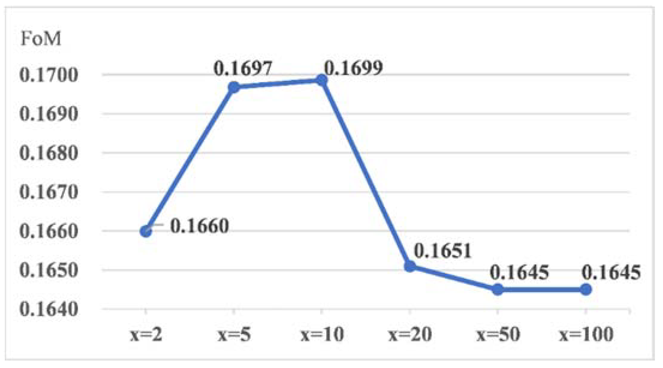
Table 7 shows the calculated results of FoM, and it can be found that the FoM reaches more than 0.1600, reflecting the high accuracy of the simulation results. In order to further analyze the relationship between the simulation results and the retrieved quantity x, as can be seen from Figure 8, the simulation accuracy first increased and then decreased as x increased; it reached its highest value when x was ten.
CBR is based on the similarity between the cases to reason; the higher the similarity, the higher the reliability of the reasoning basis. Here, it was experimentally demonstrated that the comprehensive retrieval takes into account the role of multiple geographical cases with the highest similarity. In the x geographical cases retrieved, the simulation accuracy was effectively improved when the similarity between each geographical case and the simulated case was high. However, as x increased, the similarity between the retrieved geographical cases and the simulated cases gradually decreased. Therefore, the accuracy of the inference results also decreased.

3.2. Evaluation of Effectiveness of Comprehensive Retrieval Strategy

The effectiveness of the comprehensive retrieval strategy can be analyzed by comparing the simulation accuracy of comprehensive retrieval with that of single retrieval. Using the same data, the simulation results of CBR urban growth based on a single retrieval strategy were obtained. The cases with different results under the two retrieval strategies were counted (Table 8), revealing a total of 1383 cases with different “results”. Among these, 319 correct and 1064 incorrect cases were simulated by the comprehensive retrieval strategy; 134 correct and 1249 incorrect cases were simulated by the single retrieval strategy. The accuracy of the simulation was therefore increased by 13.38% by using comprehensive retrieval. This shows that the comprehensive retrieval strategy is effective.

3.3. Contrast with the CA Model

In this paper, the CA model was compared to the CBR model to further evaluate the latter.
The CA model is a grid dynamic model that is controlled by local rules. It has no established mathematical expression. It can simulate the evolution process of the spatial patterns of urban land by setting the parameters and initial values of the simulation rules [40]. Many studies have shown that CA is not only very useful for simulating complex systems [41,42], but is also commonly used to simulate land use change. It can also effectively represent the nonlinear spatial random change process [43].
CA consists of five parts: the cell, cell space, neighborhood, time, and transformation rules. Among these, the cell is the basic unit of CA. A regular square cell is also commonly used; it can be easily combined with the raster data of a remote sensing image. Cellular space refers to the space of cellular distribution; it is mostly concentrated in two-dimensional space. Neighborhood refers to the cell that is adjacent to the current cell. In the two-dimensional square cell space, most of the surrounding eight cells are used as the cell space (molar type). The change in time is discrete, and is an important condition for triggering the change of cellular state. The cellular state at the next moment is only related to the cellular state at the current moment. The transformation rule is the core of CA [42]; this rule is used to describe the conditions or methods of cellular changes in the time domain. It can be calculated as follows:
S ( t + 1 ) = f ( S ( t ) , N x )
where S(t+1) is the state of the cell at the time t + 1, S(t) is the state of the cell at time t, and Nx is the state of the cell in the neighborhood range of cell x × x.
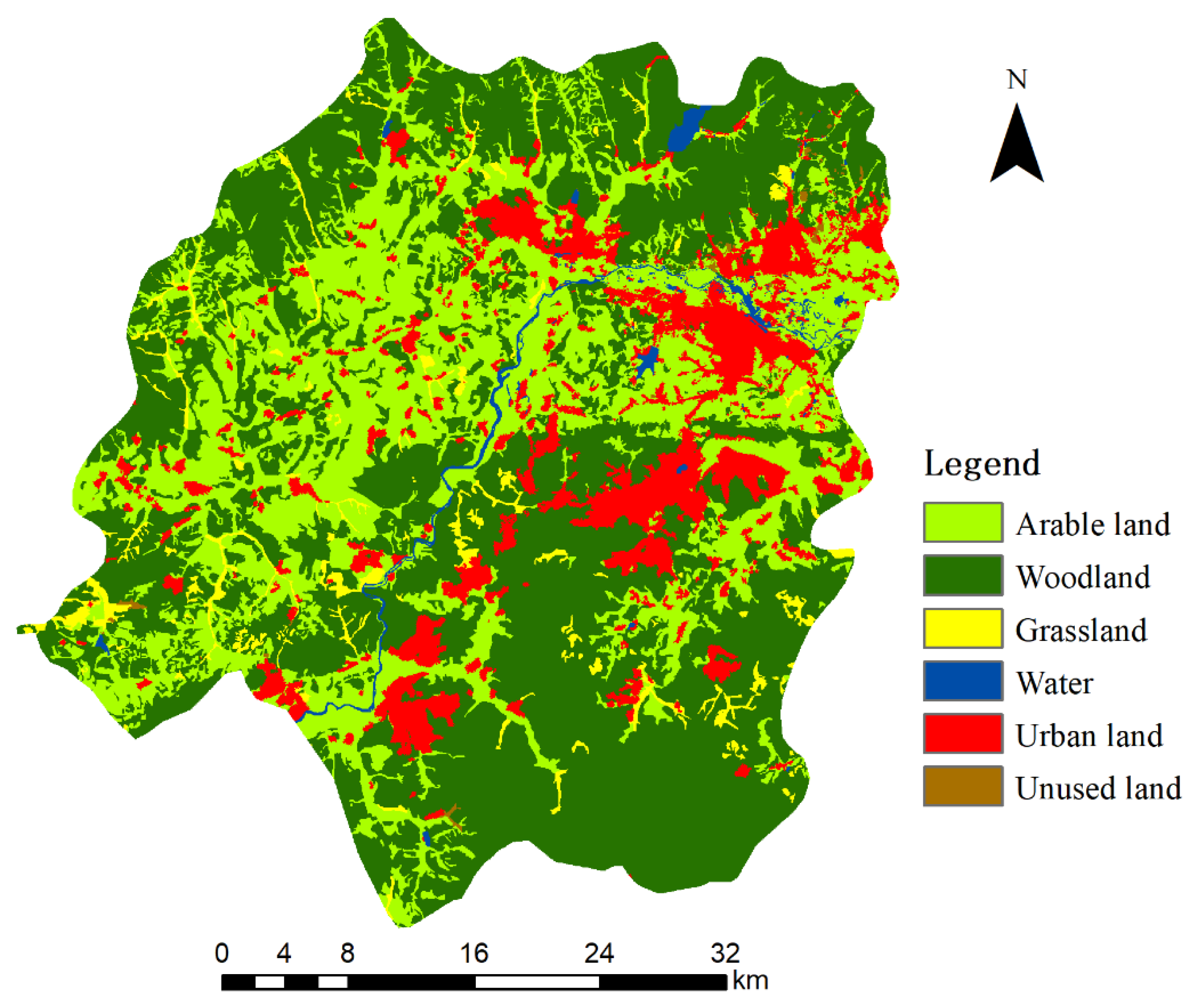
In this study, CA simulation was implemented by the Geographical Simulation and Optimization System (GeoSOS), which was proposed and developed by Professor Li Xia and their team [44]. This system is a coupled model of geographic simulation and spatial optimization; it can be used to simulate and spatially optimize changes in global land use and urban growth. The Logistic-CA module is suitable for modelling the conversion of non-urban to urban land for a single type of land use. This model uses the logistic regression method to extract rules and apply them to the simulation [45]. Using the research data mentioned above, in this study the rules were set such that arable land, woodland, grass land, and unused land could be transformed into urban land. The CA urban growth simulation result of Jixi in 2015 was obtained after 200 iterative calculations (Figure 9). Table 9 shows that the total accuracy of the CA simulation result was 96.91, and that the simulation accuracies of the urbanized and non-urbanized cases were 86.99% and 98.31%, respectively. In addition, the kappa coefficient was 84.98% and the FoM indicator was 0.148.
Comparing the CA simulation results with the urban growth CBR simulation results (Table 10) reveals that the simulation accuracy of the urban growth CBR model was higher. Further analysis of the driving mechanisms and simulation processes of these two models shows that they have the following characteristics:
(1)
CA simulation is a process based on neighborhood evolution, meaning that new urban growth land is inevitably adjacent to existing urban land. Thus, the simulation result is often affected by the cluster effect, which makes it difficult to simulate the enclave growth process and leads to a certain deviation from the actual urban pattern. Urban growth CBR simulation only considers the background conditions of each case and is not restricted by neighborhood conditions. Therefore, it can better reflect the spatial distribution trends of urban growth.
(2)
The effectiveness of CA greatly depends on the mining of transformation rules; if the rules are expressed in a too simple or too complex way, then this is not conducive to model simulation. Urban growth CBR is a kind of black-box reasoning process; it can effectively avoid the problems caused by rule mining, and its process for creating the case base is easier than CA’s process for constructing rules. From this point of view, the urban growth CBR model is simpler and easier to understand than CA.
(3)
Urban growth CBR is an empirical reasoning method, meaning that its simulation accuracy will be restricted by experience. If the number of geographical cases is too small, then it will be difficult to guarantee the model’s accuracy. At the same time, the number of cases also affects the model’s operation speed. Collecting a large number of geographical cases to improve the accuracy will decrease the model’s operation efficiency. However, CA requires less computation than urban growth CBR, and so simulation results can be obtained more quickly.

4. Conclusions

Simulating urban growth patterns is a necessary step for sustainable land use management. The major contribution of this study is that it improves the CBR model traditionally used to simulate land use changes, thereby developing a CBR model for simulating urban growth. It redefined the case expression mode, developed the idea of case comprehensive retrieval, and proposed the introduction of a method to constrain the time factor.
This model was evaluated by taking the municipal district of Jixi as the research area. It was found that when the parameter x = 10, the simulation accuracy was 97.02%, kappa was 85.51, and FoM was 0.1699. The experimental results showed good simulation effects. In addition, the influences of different parameters and the validity of the model were discussed, and the effective categories for a comprehensive retrieval strategy were outlined. Compared with the CA model, the urban growth CBR model demonstrated higher accuracy, a simpler model construction, and a better ability to reflect trends in urban growth. However, the model requires a large amount of computation and has a slow running speed, but we will mostly solve this problem in the future.
In summary, the proposed model provides a flexible, simple, and easy to understand method for studying the evolution mechanisms of urban patterns. The research results presented here can help us to understand the evolution characteristics of urban spatial patterns, provide support for scientific urban regional planning decisions, guide reasonable increases in land for construction, and promote the sustainable and healthy development of cities.

Author Contributions

Conceptualization, X.Y.; methodology, X.Y.; formal analysis, X.Y. and W.Y.; resources, X.Y. and L.L.; data curation, L.L.; writing-original draft preparation, X.Y.; writing-review & editing, X.Y.; visualization, X.Y. and W.Y.; and validation, S.Z. and H.N. All authors have read and agreed to the published version of the manuscript.

Funding

This research was funded by the Philosophy and Social Sciences Research Program of Heilongjiang Province of China (Grant No. 19JLC116), the Natural Science Foundation of Heilongjiang Province of China (Grant No. YQ2019D006), and the Fundamental Research Funds for the Provincial Universities of Heilongjiang Province of China (Grant No. 2018-KYYWF-1178, 2018-KYYWF-1179).

Institutional Review Board Statement

Not applicable.

Informed Consent Statement

Not applicable.

Data Availability Statement

Not applicable.

Acknowledgments

We thank the reviewers for their insightful and intelligent suggestions for the manuscript.

Conflicts of Interest

The authors declare no conflict of interest.

References

  1. Angel, S.; Parent, J.; Civco, D.L.; Blei, A.; Potere, D. The dimensions of global urban expansion: Estimates and projections for all countries, 2000–2050. Prog. Plann. 2011, 75, 53–107. [Google Scholar] [CrossRef]
  2. Xia, H.; Qin, Y.; Feng, G.; Meng, Q.; Cui, Y.; Song, H.; Ouyang, Y.; Liu, G. Forest Phenology Dynamics to Climate Change and Topography in a Geographic and Climate Transition Zone: The Qinling Mountains in Central China. Forests 2019, 10, 1007. [Google Scholar] [CrossRef] [Green Version]
  3. Zhou, H.; Xu, M.; Hou, R.; Zheng, Y.; Chi, Y.; Ouyang, Z. Thermal acclimation of photosynthesis to experimental warming is season-dependent for winter wheat (Triticum aestivum L.). Environ. Exp. Bot. 2018, 150, 249–259. [Google Scholar] [CrossRef] [Green Version]
  4. Yu, S.; Zhang, Z.; Liu, F.; Wang, X.; Hu, S. Urban expansion in the megacity since 1970s: A case study in Mumbai. Geocarto. Int. 2019, 1–19. [Google Scholar] [CrossRef]
  5. Seto, K.C.; Guneralp, B.; Hutyra, L.R. Global forecasts of urban expansion to 2030 and direct impacts on biodiversity and carbon pools. Proc. Natl. Acad. Sci. USA 2012, 109, 16083–16088. [Google Scholar] [CrossRef] [Green Version]
  6. Zhang, T. Land market forces and government’s role in sprawl: The case of China. Cities 2000, 17, 123–135. [Google Scholar] [CrossRef]
  7. Han, L.; Zhou, W.; Li, W. Increasing impact of urban fine particles (PM2.5) on areas surrounding Chinese cities. Sci. Rep. 2015, 5, 12467. [Google Scholar] [CrossRef] [Green Version]
  8. You, H.; Yang, X. Urban expansion in 30 megacities of China: Categorizing the driving force profiles to inform the urbanization policy. Land Use Policy 2017, 68, 531–551. [Google Scholar] [CrossRef]
  9. Meng, L.; Sun, Y.; Zhao, S. Comparing the spatial and temporal dynamics of urban expansion in Guangzhou and Shenzhen from 1975 to 2015: A case study of pioneer cities in China’s rapid urbanization. Land Use Policy 2020, 97, 104753. [Google Scholar] [CrossRef]
  10. Wu, R.; Li, Z.; Wang, S. The varying driving forces of urban land expansion in China: Insights from a spatial-temporal analysis. Sci. Total Environ. 2020, 142591. [Google Scholar] [CrossRef]
  11. Li, X.; Fan, W.; Wang, L.; Luo, M.; Yao, R.; Wang, S.; Wang, L. Effect of urban expansion on atmospheric humidity in Beijing-Tianjin-Hebei urban agglomeration. Sci. Total Environ. 2021, 759, 144305. [Google Scholar] [CrossRef]
  12. Liu, J.; Jiao, L.; Zhang, B.; Xu, G.; Yang, L.; Dong, T.; Xu, Z.; Zhong, J.; Zhou, Z. New indices to capture the evolution characteristics of urban expansion structure and form. Ecol. Indic. 2021, 112, 107302. [Google Scholar] [CrossRef]
  13. Jafari, M.; Majedi, H.; Monavari, S.M.; Alesheikh, A.A.; Zarkesh, M.K. Dynamic simulation of urban expansion through a CA-Markov model Case study: Hyrcanian region, Gilan, Iran. Eur. J. Remote Sens. 2016, 49, 513–529. [Google Scholar] [CrossRef] [Green Version]
  14. Yao, Y.; Ma, L.; Che, X.; Dou, H. Simulation study of urban expansion under ecological constraint—Taking Yuzhong County, China as an example. Urban. For. Urban. Green 2021, 57, 126933. [Google Scholar] [CrossRef]
  15. Cheng, J.; Masser, I. Understanding Spatial and Temporal Processes of Urban Growth: Cellular Automata Modelling. Environ. Plann. B Plann. Des. 2004, 31, 167–194. [Google Scholar] [CrossRef]
  16. Firozjaei, M.K.; Sedighi, A.; Argany, M.; Jelokhani-Niaraki, M.; Arsanjani, J.J. A geographical direction-based approach for capturing the local variation of urban expansion in the application of CA-Markov model. Cities 2019, 93, 120–135. [Google Scholar] [CrossRef]
  17. Liang, X.; Liu, X.; Li, X.; Chen, Y.; Tian, H.; Yao, Y. Delineating multi-scenario urban growth boundaries with a CA-based FLUS model and morphological method. Landsc. Urban. Plan. 2018, 177, 47–63. [Google Scholar] [CrossRef]
  18. Tian, G.; Ouyang, Y.; Quan, Q.; Wu, J. Simulating spatiotemporal dynamics of urbanization with multi-agent systems—A case study of the Phoenix metropolitan region, USA. Ecol. Modell 2010, 222, 1129–1138. [Google Scholar] [CrossRef]
  19. Zhang, H.; Jin, X.; Wang, L.; Zhou, Y.; Shu, B. Multi-agent based modeling of spatiotemporal dynamical urban growth in developing countries: Simulating future scenarios of Lianyungang city, China. Stoch Environ. Res. Risk Assess. 2015, 29, 63–78. [Google Scholar] [CrossRef]
  20. He, X.; Mai, X.; Shen, G. Delineation of Urban Growth Boundaries with SD and CLUE-s Models under Multi-Scenarios in Chengdu Metropolitan Area. Sustainability 2019, 11, 5919. [Google Scholar] [CrossRef] [Green Version]
  21. Luo, G.; Yin, C.; Chen, X.; Xu, W.; Lu, L. Combining system dynamic model and CLUE-S model to improve land use scenario analyses at regional scale: A case study of Sangong watershed in Xinjiang, China. Ecol. Complex. 2010, 7, 198–207. [Google Scholar] [CrossRef]
  22. Liu, Z.; Yang, Y.; He, C.; Tu, M. Climate change will constrain the rapid urban expansion in drylands: A scenario analysis with the zoned Land Use Scenario Dynamics-urban model. Sci. Total Environ. 2019, 651, 2772–2786. [Google Scholar] [CrossRef]
  23. Du, Y.; Wen, W.; Cao, F.; Ji, M. A case-based reasoning approach for land use change prediction. Expert Syst. Appl. 2010, 37, 5745–5750. [Google Scholar] [CrossRef]
  24. De Mantaras, R.L.; McSherry, D.; Bridge, D.; Leake, D.; Smyth, B.; Craw, S.; Faltings, B.O.I.; Maher, M.L.; Cox, M.T.; Forbus, K.; et al. Retrieval, reuse, revision and retention in case-based reasoning. Knowl. Eng. Rev. 2005, 20, 215–240. [Google Scholar] [CrossRef] [Green Version]
  25. Du, Y.; Ge, Y.; Lakhan, V.C.; Sun, Y.; Cao, F. Comparison between CBR and CA methods for estimating land use change in Dongguan, China. J. Geogr. Sci. 2012, 22, 716–736. [Google Scholar] [CrossRef]
  26. Karen, K. Case-Based Reasoning: An Introduction. Expert Syst. Appl. 1993, 6, 3–8. [Google Scholar] [CrossRef]
  27. Liao, Z.; Zhou, C.; Tian, W.; Hu, T.; Guo, R. CBR-based integration of a hydrodynamic and water quality model and GIS-a case study of Chaohu City. Environ. Sci. Pollut. Res. 2019, 26, 6436–6449. [Google Scholar] [CrossRef] [PubMed] [Green Version]
  28. Huang, K.; Nie, W.; Luo, N. Scenario-Based Marine Oil Spill Emergency Response Using Hybrid Deep Reinforcement Learning and Case-Based Reasoning. Appl. Sci. 2020, 10, 5269. [Google Scholar] [CrossRef]
  29. Somi, S.; Gerami, S.N.; Fayek, A.R. Framework for Risk Identification of Renewable Energy Projects Using Fuzzy Case-Based Reasoning. Sustainability 2020, 12, 5231. [Google Scholar] [CrossRef]
  30. Liu, W.; Wang, S.; Zhou, Y.; Wang, L.; Zhu, J.; Wang, F. Lightning-caused forest fire risk rating assessment based on case-based reasoning: A case study in DaXingAn Mountains of China. Nat. Hazards 2015, 81, 347–363. [Google Scholar] [CrossRef]
  31. Machado, D.; de Menezes, M.D.; Silva, S.; Curi, N. Transferability, accuracy, and uncertainty assessment of different knowledge-based approaches for soil types mapping. Catena 2019, 182, 104134. [Google Scholar] [CrossRef]
  32. Dou, J.; Chang, K.-T.; Chen, S.; Yunus, A.; Liu, J.-K.; Xia, H.; Zhu, Z. Automatic Case-Based Reasoning Approach for Landslide Detection: Integration of Object-Oriented Image Analysis and a Genetic Algorithm. Remote Sens. 2015, 7, 4318–4342. [Google Scholar] [CrossRef] [Green Version]
  33. Du, Y.; Wu, D.; Liang, F.; Li, C. Integration of case-based reasoning and object-based image classification to classify SPOT images: A case study of aquaculture land use mapping in coastal areas of Guangdong province, China. GIsci. Remote Sens. 2013, 50, 574–589. [Google Scholar] [CrossRef]
  34. Liu, X.; Ma, L.; Li, X.; Ai, B.; Li, S.; He, Z. Simulating urban growth by integrating landscape expansion index (LEI) and cellular automata. Int. J. Geogr. Inf. Sci. 2014, 28, 148–163. [Google Scholar] [CrossRef]
  35. Liang, X.; Liu, X.; Li, D.; Zhao, H.; Chen, G. Urban growth simulation by incorporating planning policies into a CA-based future land-use simulation model. Int. J. Geogr. Inf. Sci. 2018, 32, 2294–2316. [Google Scholar] [CrossRef]
  36. Holt, A. Applying case-based reasoning techniques in GIS. Int. J. Geogr. Inf. Sci. 1999, 13, 9–25. [Google Scholar] [CrossRef]
  37. McSherry, D. The inseparability problem in interactive case-based reasoning. Knowl. Based Syst. 2002, 15, 293–300. [Google Scholar] [CrossRef]
  38. Dong, Q.; Ai, X.; Cao, G.; Zhang, Y.; Wang, X. Study on risk assessment of water security of drought periods based on entropy weight methods. Kybernetes 2010, 39, 864–870. [Google Scholar] [CrossRef]
  39. Pontius, R.G.; Huffaker, D.; Denman, K. Useful techniques of validation for spatially explicit land-change models. Ecol. Model. 2004, 179, 445–461. [Google Scholar] [CrossRef]
  40. Tong, X.; Feng, Y. A review of assessment methods for cellular automata models of land-use change and urban growth. Int. J. Geogr. Inf. Sci. 2020, 34, 866–898. [Google Scholar] [CrossRef]
  41. Wolfram, S. Cellular automata: A model of complexity. Nature 1984, 31. [Google Scholar] [CrossRef]
  42. Li, X.; Liu, X. An extended cellular automaton using case--based reasoning for simulating urban development in a large complex region. Int. J. Geogr. Inf. Sci. 2006, 20, 1109–1136. [Google Scholar] [CrossRef]
  43. Liu, X.; Liang, X.; Li, X.; Xu, X.; Ou, J.; Chen, Y.; Li, S.; Wang, S.; Pei, F. A future land use simulation model (FLUS) for simulating multiple land use scenarios by coupling human and natural effects. Landsc. Urban. Plan. 2017, 168, 94–116. [Google Scholar] [CrossRef]
  44. Li, X.; Shi, X.; He, J.; Liu, X. Coupling Simulation and Optimization to Solve Planning Problems in a Fast-Developing Area. Ann. Assoc. Am. Geogr. 2011, 101, 1032–1048. [Google Scholar] [CrossRef]
  45. Wu, F. Calibration of stochastic cellular automata: The application to rural-urban land conversions. Int. J. Geogr. Inf. Sci. 2002, 16, 795–818. [Google Scholar] [CrossRef]
Figure 1. Location map of the study area.
Sustainability 13 06146 g001
Figure 2. Case expression and collection.
Sustainability 13 06146 g002
Figure 3. Basic case retrieval strategy.
Sustainability 13 06146 g003
Figure 4. Comprehensive case retrieval strategy.
Sustainability 13 06146 g004
Figure 5. Case constraint process.
Sustainability 13 06146 g005
Figure 6. The urban growth case-based reasoning (CBR) model procedure.
Sustainability 13 06146 g006
Figure 7. Simulated and actual urban development of Jixi in 2015.
Sustainability 13 06146 g007
Figure 8. The relationship between x and FoM.
Sustainability 13 06146 g008
Figure 9. Simulation result of urban growth based on cellular automata (CA).
Sustainability 13 06146 g009
Table 1. Urban growth indicators and process mode.
IndexProcess Mode
DEMASTER GDEMV2 digital elevation products, grid size of 30 m × 30 m
Distance to the city center
(Dcenter1)
Taking Jixi Municipal Government as the center, the distance between all grid cells and the center is obtained by using “Euclidean distance” function
Distance to the district center of gravity
(Dcenter2)
Obtain the nearest distance of all grid cells to the center of gravity of each district using “Euclidean distance” function
Distance to the city edge
(Dedge)
Obtain the distance of all grid cells to the nearest urban land using “Euclidean distance” function
Distance to the mining area
(Dmining)
Obtain the distance of all grid cells to the nearest mining area using “Euclidean distance” function
Distance to the water
(Dwater)
Obtain the distance of all grid cells to the nearest water using “Euclidean distance” function
Distance to the railway
(Drailway)
Obtain the distance of all grid cells to the nearest railway using “Euclidean distance” function
Distance to the highway
(Droad)
Obtain the distance of all grid cells to the nearest highway using “Euclidean distance” function
Table 2. Collection numbers of geographical case database (GCDB) groups (cells).
Initial StateArable LandWoodlandGrass LandUnused Land
urbanized15,09614,1452248286
Non-urbanized15,04615,05415,0157007
Cases30,14229,19917,2637293
Table 3. Collection numbers of simulated case database (SCDB) groups (cells).
Initial StateArable LandWoodlandGrass LandUnused Land
Cases631,7171,224,34062,1684419
Table 4. Index weights for each group of cases.
IndexDEMDcenter1Dcenter2DedgeDminingDwaterDrailwayDroad
Arable land0.04510.04580.03490.13580.05700.12110.10910.1027
Woodland0.01930.02550.03270.10310.06610.08600.08020.0907
Grass land0.02230.02410.02010.10230.07790.12200.06280.0679
Unused land0.03880.09740.04610.16560.03730.09810.11990.0988
Table 5. Quantity demand for urban growth during 2010−2015 (cells).
Initial StateArable LandWoodlandGrass LandUnused Land
QD37,38210,897838391
Table 6. Simulation accuracies of the CBR model.
x = 2
Simulated Non-UrbanSimulated UrbanAccuracy
Actual non-urban2,063,87335,41298.31%
Actual urban35,831240,33487.03%
Total accuracy 97.00%
x = 5
Simulated non-urbanSimulated urbanAccuracy
Actual non-urban2,064,14135,14498.33%
Actual urban35,563240,60287.12%
Total accuracy 97.02%
x = 10
Simulated non-urbanSimulated urbanAccuracy
Actual non-urban2,064,15435,13198.33%
Actual urban35,550240,61587.13%
Total accuracy 97.02%
x = 20
Simulated non-urbanSimulated urbanAccuracy
Actual non-urban2,063,80835,47798.31%
Actual urban35,896240,26987.00%
Total accuracy 97.00%
x = 50
Simulated non-urbanSimulated urbanAccuracy
Actual non-urban2,063,76735,51898.31%
Actual urban35,937240,22887.00%
Total accuracy 96.99%
x = 100
Simulated non-urbanSimulated urbanAccuracy
Actual non-urban2,063,78935,49698.31%
Actual urban35,915240,25087.00%
Total accuracy 96.99%
Table 7. The kappa and figure of merit (FoM) of the CBR model simulation.
Retrieval Quantityx = 2x = 5x = 10x = 20x = 50x = 100
Kappa85.39%85.50%85.51%85.37%85.35%85.35%
FoM0.16600.16970.16990.16510.16450.1645
Table 8. Accuracy comparison between comprehensive retrieval and single retrieval.
Retrieval StrategyComprehensiveSingle
Correct319134
Incorrect10641249
Accuracy23.07%9.69%
Table 9. Simulation accuracies of the CA model.
Simulated UrbanSimulated Non-UrbanAccuracy
Actual urban240,12436,04186.99%
Actual non-urban35,6222,063,66398.31%
Total accuracy 96.99%
Table 10. Comparison of accuracy of urban growth CBR and CA simulation results.
AccuracyKappaFoM
CBR (x = 10)97.02%85.51%0.170
CA96.91%84.98%0.148
Publisher’s Note: MDPI stays neutral with regard to jurisdictional claims in published maps and institutional affiliations.