Abstract
Total height is one of the basic morphometric tree variables included in all forest management inventories, because it is connected with several forest processes and functions related to the estimation of the woody tree volume and sustainable forest yield. The current research, based on a total sample of 1059 measured Black pine (Pinus nigra Arn.) trees from Cyprus, is an attempt to explore the biological processes related to the tree height allometry of this species and develop a generalized mixed-effects model for tree height prediction. The proposed model, with three additional basic covariates and two random parameters, explained almost 96% of the height variance. The model results showed that although competition and site-connected variables affected the total height, it was the crown base height that explained, to a large degree, the height expression. Through the mixed-effects modeling approach it was possible to explore the complex biological processes related to the tree allometry of Black pine and depict those within a mathematical formulation. The proposed generalized model decreased the error significantly, and therefore it can be used for operational forest management purposes. However, for marginal predictions, use of only the fixed part of the basic model could suffice, since this also provided unbiased parameter estimates.
1. Introduction
Total height is one of the basic morphometric tree variables. It directly affects the woody tree volume and sustainable forest yield, and it is currently included in all forest management inventories and plans. It has been connected to the site index [1], light capture [2], growth dynamics and succession [3], carbon sequestration [4] and tree stability [5]. From an ecological perspective, total height is a fundamental component of processes and functions at a tree or at an ecosystem level [6]. It reflects the outcome of the combined effect of several endogenous and exogenous variables that may be expressed through complex models for height prediction.
The diameter at breast height is a key element in forest inventories [7] and the main covariate in linear or nonlinear basic models for height prediction. However, the height–diameter relationship deviates between different forest stands [8]. In order to solve this problem, additional covariates were introduced in the proposed models, thus leading to the development of models suitable for regional use [9]. Temesgen and von Gadow [10] introduced the term “generalized” to describe the height–diameter curve with additional variables at the stand level. The generalized models have improved the height prediction accuracy for large forests, and they have allowed the description of the ecological connections between the variables included in the models. Through this, the researchers managed to explore the ecological processes behind the height expression at various levels, providing ecological explanations for the largest part of height variations [11].
The development of generalized models is currently based on two approaches [12]. According to the first approach, the parameters of the basic models are expressed using mathematical forms of the stand variables [13]. Usually, a preliminary comparison between the height and the independent variable(s) is performed prior to the model fitting. The second approach recommends the direct input of the additive covariates into the model [12]. However, regardless of the approach followed, the implementation of the generalized models is not fully adequate due to the fact that similar stand characteristics assume similar height–diameter curves [14]. Moreover, the inclusion of a large number of independent variables may lead to over-parameterization problems.
The mixed-effects approach provided new perspectives on height modeling procedures [15]. These types of models are recommended when analysis should be carried out on nested data from tree height observations obtained from installed sample plots, which usually present a lack of independence between them [16]. Mixed-effects models are mainly composed of two parts, the fixed-effects part that refers to the properties of the entire population and the random-effects part that is associated with the individual properties of separate sample plots [17]. Their random part may also capture the effect of independent variables that are not included in the fitted model [18]. Thus, the mixed-effects modeling technique is a powerful tool for the development of generalized models and the ecological exploration of processes and functions behind the tree height allometry.
The basic aims of the current study were as follows: (i) the development of a generalized mixed-effects model for the tree height prediction of Black pine (Pinus nigra Arn.) and (ii) the exploration of the ecological process of each covariate included in the proposed model of Black pine height allometry. For the model development and evaluation in terms of fitting ability, field data derived from the natural even-aged Black pine forests of Troodos National Forest Park in Cyprus were used. In this region, Black pine forms a separate population and is characterized by geographical isolation. Despite the fact that it has been studied both in Turkey [19] and in Greece [20], the Cyprus populations have never been studied before and they constitute the focus of the current study.
2. Materials and Methods
Black pine, a native pine species of the Troodos Mountains in Cyprus, is often characterized as a mountain pine in the wider region. At lower altitudes it is intermingled with Calabrian pine (Pinus brutia Ten.) and dominates above 1400 m of elevation [21], forming pure and naturally regenerated even-aged stands. These types of forests cover a total area of 9147 hectares at the center of the south and south-west parts of the island (Figure 1).
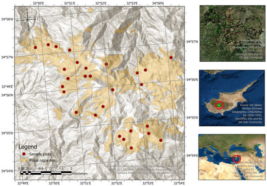
Figure 1.
The Troodos Mountains study area and the spatial distribution of the sample plots.
In higher locations, the Black pine is intermingled with Juniper (Juniperus foetidissima Willd.) as a secondary species. The soil is shallow, residual and skeletal from the underlying diabase and gabbro, becoming stiffer in mild slopes [22]. The meteorological data from the nearest station in Prodromos area indicate that the mean annual precipitation is about 790 mm, and the mean annual temperature is 13 °C.
2.1. Sampling
The spatial information on the Black pine distribution in the Troodos Mountains was provided by the Department of Forests of the Cyprus Ministry of Agriculture, Rural Development and Environment in a GIS file format (shapefile). Using the “create random points” module in a GIS environment, 30 potential locations for field measurements were identified. However, only 28 sample plots were installed in the field, since access in two of the locations was not feasible due to physical obstacles. The sample units (plots) were circular, with a radius of 12.62 m in a horizontal projection, covering a total area of 500 m2 each. Within each plot, the diameter at breast height (1.30) (dbh) was measured with a caliper.
The total height (h) and the crown base height (cbh) were measured using a LaserAce hypsometer (Trimble, Sunnyvale, CA, USA). The crown width (cw) was measured using the “canopy spread” module of the same instrument in two vertical directions. The total sample included 1059 Black pine trees and the descriptive statistics of the main measured variables are presented in Table 1. Trees with damaged or broken tops were excluded from the sample.

Table 1.
Descriptive statistics of the data used for model development.
Based on the measurements at tree level, several stand-based indexes were estimated covering basic aspects of the soil productivity and competition regimes within the forests stands. The dominant height (hdom) and the dominant diameter (ddom) were calculated from the mean values of the 100 thickest trees per hectare or equally proportional to the plot size [23]. The estimated density indexes included the basal area per hectare (m2·ha−1), the number of trees (stems) per hectare (N·ha−1), the quadratic mean diameter (qmd), the stand density index (sdi) [24], the relative spacing index (rsi) [25] and the spacing coefficient (sc) [26,27]. Their mathematical expressions are as follows:
where n is the number of the estimated stems per hectare at plot level. The crown competition factor (ccf) [28] was calculated using a quantile regression for a nonlinear mixed- effects model of the maximum crown width from the 95th percentile points, based on the qrNLMM package [29] in the R (cran) environment. The fitted model was of the simple power form y = axb according to the findings of Raptis et al. [18] for Black pine in Greece, where y is the maximum crown width, x is the diameter and a, b are the fixed parts of the mixed-effects model.
2.2. Statistical Analysis
2.2.1. Basic Model Selection
For the basic model selection, 5 fundamental nonlinear models for height–diameter allometry were selected for evaluation.
The selected models (Table 2) included only 2-parameter nonlinear forms due to convergence problems experienced during model fitting. Taking into consideration the hierarchical nested structure of the available data, an OLS fitting would lead to underestimates of the covariance matrix of the parameter estimates and the residual variance of the regression equation [16]. Due to this limitation, instead of an OLS fitting procedure, it was decided mixed-effects modeling at two different levels would be used, for the simple model selection and for the generalized expanded form. A detailed description of the nonlinear mixed-effects modeling technique is provided by Calama and Montero [30]. All the model parameters were assumed to contain a random part and their variances were reported. On condition of almost zero variance, the parameter was regarded as fixed. In case of convergence problems, the mixed parameters were reduced gradually [17].
Table 2.
2-Parameter models and mathematical forms of mixed-effects.
The selection of the basic model was based on the following five criteria of good fit: (i) the Root Mean Square Error (RMSE); (ii) the Fitting Index (FI) that was based on the R squared mathematical expression [36]; (iii) the Akaike information criterion [37], which penalizes the number of the model’s parameters; (iv) the Bayesian information criterion, which also penalizes the total number of the model’s parameters [38] and (v) the mean prediction bias. Their mathematical expressions are as follows:
where hj, and represent the measured, estimated and mean values of the total height variable of the jth observation, respectively, n represents the number of observations forming the total sample, p represents the number of estimated model parameters and L represents the likelihood of the fitted model.
In case of an unequal error variance, a function to regulate it was applied in a power, exponential or constant/power mathematical form by linking the variance with a predictor. Assuming that the i indicator represents the different plots and the j indicator each tree within the plot, the variance functions that were tested were the following:
where δ, δ1 and δ2 are the parameters to be estimated and is the independent predictor to stabilize the variance of the within-plot heteroscedasticity. Since dbh has been successfully used as an independent predictor to regulate the variance in relevant research works for Black pine [18,39], it was decided that the same method would be followed. The most suitable function along with the most appropriate predictor was determined by visual inspection of the residuals and the results of the likelihood ratio test (LTR), [40] the AIC and the BIC criteria, as these have been incorporated in the anova function for nested models [17]. According to the same authors [17], the anova function, when two or more arguments of fitted models are used, produces likelihood ratio tests, which compare the models and provide the p value from the distribution, for k2−k1 degrees of freedom, with ki representing the number of parameters to be estimated in model i. In order to test the normality assumption of the residuals, the graphical Q–Q plot method was used.
2.2.2. Generalized Model Expansion
The selected model was the basis for developing a reliable generalized model and explaining height allometry on an ecological basis in the second phase. The development of the generalized model was based on the correlation between the plot-specific parameters of the simple model and the variables at stand level [23]. The estimation of the plot-specific parameters was based on the nlsList function of the nlme library. It is an alternative method for model expansion, closely linked to mixed-effects modeling. Through this procedure, specific covariates at tree and stand level were incorporated in the expanded generalized model in order to reduce the random variance of the simple model parameters.
At the final stage, the generalized form was expanded to a generalized mixed-effects model in order to explain the largest possible portion of height variance. Again, all the parameters were assumed to contain a random part [41] as long as convergence was attainable. Otherwise, the number of the mixed parameters was reduced gradually until convergence was achieved. In a case of convergence, the mixed parameters were further reduced, and the nested models were compared using the anova function. In a case of no significant difference between the nested models (likelihood ratio statistic p-value > 0.05), the simplest form was selected [17]. Finally, the graphical solution was preferred to evaluate the fitting performance of the selected model against the total dataset of height–diameter observations, for both types of models.
2.2.3. Ecological Explanations
The effect of each covariate of the generalized model was evaluated graphically, using five equal intervals between the covariate bounds from Table 1, while using the mean values of the other in two-dimensional charts [42]. Based on the chart form, ecological explanations were attempted in order to investigate the processes behind tree height expression, along with the other competition or productivity-related independent variables.
2.2.4. Analysis
For the statistical analysis, open-source R software was used [43]. For the mixed-effects model fitting along with the nlsList and the anova functions, the nlme library [17] was implemented. The residual analysis was based on the lmfor package [14] and the graphical illustrations on the ggplot2 package.
3. Results
The scatterplot of the height against the diameter is presented in Figure 2. During model fitting, serious convergence problems were detected when all of the parameters were assumed to be mixed in 3-parameters models. The mixed-effects parameters were reduced but still convergence problems were detected in two sample plots, despite the different combinations of the initial parameter estimates, which were further confirmed by the nlsList function. Hence, the 2-parameter models were preferred since they presented an increased convergence ability.
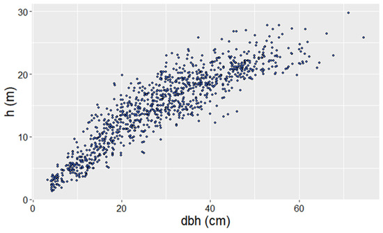
Figure 2.
Scatterplot of the diameter (dbh) against height (h), Pinus nigra Arn. National Forest Park of Troodos, Cyprus.
The Naslund’s M1 model managed to converge when both parameters were assumed to include a random part and it presented the best fittings compared to the other models (Table 3).
Table 3.
Fitting performance of the 2-parameter mixed models.
The M1 model managed to predict almost 92% of the height variance according to the reported Fitting Index and it presented the lowest error between the tested models (Table 3). However, convergence problems emerged when other 2-parameter models were tested, such as Curtis’ [3] model. Figure 3 depicts the 95% confidence intervals on the coefficients of the M1 model fitted to 28 sample plots.
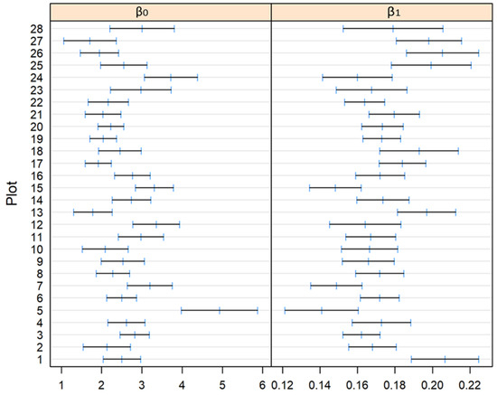
Figure 3.
The 95% confidence intervals on the coefficients (β0,1) of the Näslund’s model (M1) fitted to the total number of sample plots, Pinus nigra Arn. National Forest Park of Troodos, Cyprus.
Based on those coefficients, the M1 graphical representation (“spaghetti” chart) (Figure 4) confirms the good fitting performance of the M1 mixed-effects model.
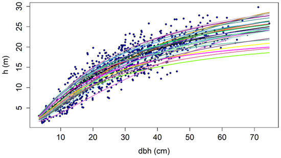
Figure 4.
“Spaghetti” chart of the Näslund’s model (M1) fitting performance against the observations of the total sample, where h is the total height and dbh is the diameter at breast height, Pinus nigra Arn. National Forest Park of Troodos, Cyprus.
The total sample and the within-group predictions against the height–diameter observations per plot (Figure 5) further configure the good performance of the suggested model, since the within-group predictions are in close agreement with the observed concentrations.
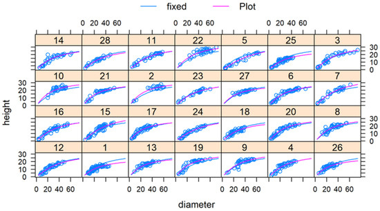
Figure 5.
Total sample predictions (fixed lines), within-group predictions (plot lines) and height–diameter observations per plot. The numbers on top correspond to the plot number, Pinus nigra Arn. National Forest Park of Troodos, Cyprus.
In addition, the visual inspection of the residuals revealed no obvious heteroscedastic trends. However, when an exponential-function form was used for residual regulation (Table 4 and Figure 6), the model was improved significantly according to the anova function (p < 0.01).
Table 4.
Comparison of variance functions with M1 mixed model.
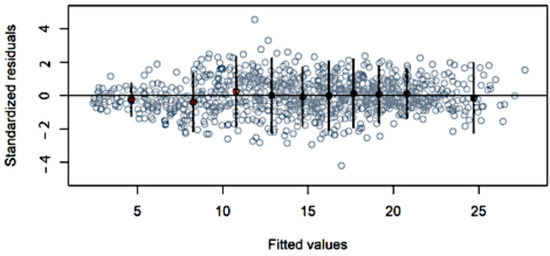
Figure 6.
Standardized residual plot for the M1 mixed-effects model after weighting. The large dots represent the mean values of the residuals according to ten classes. The thick and thin vertical lines represent the 95% confidence interval of the class mean and of one observation (mean ± SD), respectively. The red color indicates the lines that do not cross the base line at y = 0, Pinus nigra Arn. National Forest Park of Troodos, Cyprus.
Hence, the final form of the basic model was as follows:
The graphical interpretation of the Q–Q plot (Figure 7) revealed that the residuals did not decline significantly from a straight line, and the normality assumption holds.
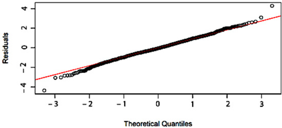
Figure 7.
Normal Q–Q plot of the weighted M1 mixed-effects model, Pinus nigra Arn. National Forest Park of Troodos, Cyprus.
The final M1 model’s parameters and fitting statistics are presented in Table 5. Assuming independence between the observations, the error of the corresponding OLS model was equal to 2.325 m, and while using only the fixed part of the model, the error was slightly increased to 2.752 m, which was expected. However, the mixed-effects models can be adjusted to each sample plot using a small sample of trees per plot, reducing the prediction error to a large extent.
Table 5.
Estimated parameters and fitting statistics of the basic mixed model (M1).
The 95th quantile regression for nonlinear mixed-effects modeling of the maximum crown width to estimate the ccf, provided the following equation:
Figure 8 presents the correlation between the model (M1) parameters and the basic variables at the plot level.
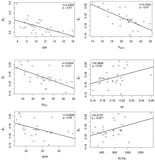
Figure 8.
Correlations between stand-level parameters (β0,1) and basic variables at the plot level. The cbh is the mean crown base height, the hdom and the ddom are the dominant height and diameter, correspondingly, the rsi is the relative spacing index, the qmd is the quadratic mean diameter and N/ha is the number of stems, Pinus nigra Arn. National Forest Park of Troodos, Cyprus.
The β0 parameter was negatively correlated with cbh (r = −0.539, p < 0.01), whereas the β1 parameter was negatively correlated with hdom (r = −0.703, p < 0.01), ddom (r = −0.650, p < 0.01) and qmd (r = −0.465, p < 0.01), and positively correlated with rsi (r = 0.385, p < 0.05) and N/ha (r = 0.417, p < 0.05). However, the ccf did not correlate with any of the two parameters.
For the development of the generalized form, the correlated variables were introduced into the model and their effect was assessed using the significance of the associated parameter (approximate t-statistic). Furthermore, the number of the inherent variables was intently tested to avoid any overfitting that could possibly occur. The hdom and the ddom at the stand level, along with the cbh at the tree level, improved the model’s performance significantly and they are proposed as additional covariates for Black pine height predictions. Despite the fact that the cbh at the plot level was correlated with β0, the inclusion of cbh at the tree level provided more accurate predictions and it was retained. The other variables were not associated with a significant parameter within the model, and they were not included in its final form. The relationships of the response variable and the covariates in the final model are presented in Figure 9, Figure 10 and Figure 11 and the form of the generalized model (G1) is as follows:
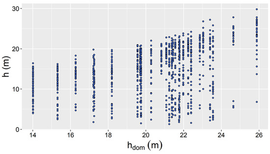
Figure 9.
Scatterplot of the dominant height (hdom) against height (h), Pinus nigra Arn. National Forest Park of Troodos, Cyprus.
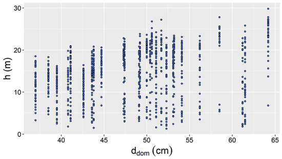
Figure 10.
Scatterplot of the dominant diameter (ddom) against height (h), Pinus nigra Arn. National Forest Park of Troodos, Cyprus.
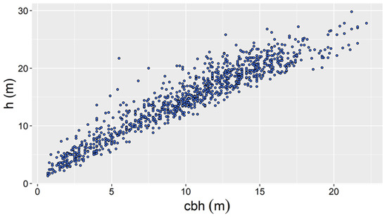
Figure 11.
Scatterplot of the crown base height (cbh) against height (h), Pinus nigra Arn. National Forest Park of Troodos, Cyprus.
In the second phase, two of the five total parameters were expanded as mixed-effects and the model was checked for heteroscedasticity by linking variance with one candidate function. The model converged when β0 and β1 were assumed as mixed and the final form was (GM1), as follows:
Table 6 presents the comparison of variance functions with the generalized mixed model (GM1). The power function presented the best results, and it was selected to regulate GM1 error’s variance.
Table 6.
Comparison of variance functions with GM1 mixed model.
Hence, the final model becomes the following:
The model’s parameter estimates, along with the fitting statistics, are shown in Table 7.
Table 7.
Estimated parameters and fitting statistics of the generalized mixed model (GM1).
The residual and the Q–Q plot are presented in Figure 12 and Figure 13, respectively. From a visual inspection, no heteroscedastic trends were detected; neither was a significant deviation from the straight line observed.
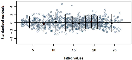
Figure 12.
Standardized residual plot for the generalized mixed-effects model GM1 after weighting with power function, Pinus nigra Arn. National Forest Park of Troodos, Cyprus.
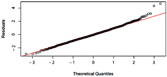
Figure 13.
Normal Q–Q plot of the weighted GM1 mixed-effects model, Pinus nigra Arn. National Forest Park of Troodos, Cyprus.
Figure 14, Figure 15 and Figure 16 depict the separate contribution of each covariate of the model in a total height allometry of Black pine trees in Cyprus. The curves were placed on a two-dimensional chart for evaluation.
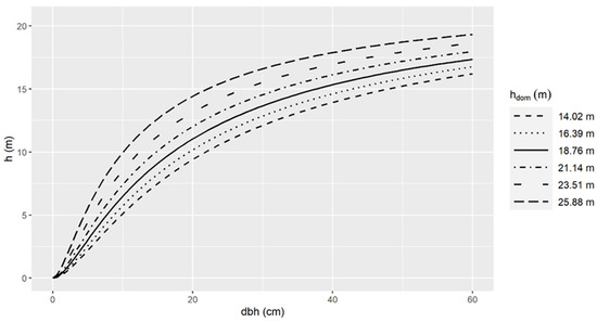
Figure 14.
Graphical representation of the effect of the dominant height (hdom) on the total tree height (h), Pinus nigra Arn. National Forest Park of Troodos, Cyprus.
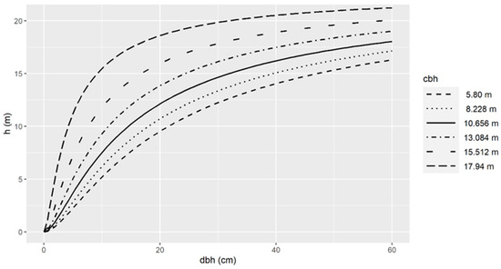
Figure 15.
Graphical representation of the effect of the crown base height (cbh) on the total tree height (h) Pinus nigra Arn. National Forest Park of Troodos, Cyprus: The effect is valid when h ≤ cbh.
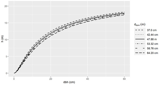
Figure 16.
Graphical representation of the effect of the dominant diameter (ddom) on the total tree height (h), Pinus nigra Arn. National Forest Park of Troodos, Cyprus.
4. Discussion
The Näslund function, which has been used for several other species due to its adequate flexibility [1], presented good fitting ability for Black pine height predictions too. Mehtätalo et al. [14] suggested the Näslund function as the best among other 2-parameter models for height–diameter mixed-effects modeling, while Sharma et al. [44] used it for height predictions of conifer and broadleaved species in the central Czech Republic. Schmidt et al. [45] also used the linear transformation of M1 model for height predictions of Scots pine (Pinus sylvestris) in Estonia. Due to the shade-intolerance and the even-aged structure of the Black pine forest stands, special conditions have been generated in the Troodos Mountains that reflect the absence of small diameter trees in the understory of some of the stands. This actually prevented some models from converging, while the Näslund function managed to converge mainly due to its parsimony and ability to be linearized from a mathematical perspective. Overall, the suggested generalized model (GM1) explained almost 96% of the height variance (Table 7). This can be attributed to the flexibility of the basic model, the introduced additional covariates and the random effect of the two model parameters. The remaining 4% of unexplained height variance can be attributed to variables or factors that are not included in the proposed model. Further improvements using additional covariates may lead to overfitting conditions due to an increased complexity. Therefore, the unexplained portion was judged to be quite small and the height allometry well captured by the GM1 generalized mixed-effects model.
From a modeling process perspective, the additional covariates are critical as far as the model’s biological validity is concerned. In a relevant study, Sharma and Zhang [46] used the stand basal area (m2·ha−1) and the stand density (n·ha−1) to explain the height allometry of both Jack pine (Pinus banksiana) and Black spruce (Picea mariana) in Canada. Gómez-García et al. [47] incorporated the dominant height, the number of stems and the dominant diameter in a mixed-effect model to develop a generalized model for the height estimation of maritime pine (Pinus maritima) stands in Portugal, while Sharma and Breidenbach [1] introduced dominant height and diameter into Näslund’s function to model the height variable of Scots pine (Pinus sylvestris), Norway spruce (Picea abies) and downy birch (Betula pubescens) in Norway. In general terms, the proposed covariates in each of the forming modeling procedures were related to the site productivity, the competition status and the development stage of forest stands and explained effectively the height variance for different tree species, which is in agreement with the current study.
The Site Index (SI) reflects the combined effect of physical and ecological factors, which are expressed though the site’s ability to support tree growth [48]. It is closely linked with the hdom, since it is estimated from the mean height of the largest trees at a reference age [49]. The effect of hdom on the height expression of Black pine trees suggests that the height of trees with an equal height to crown base height, grown in similar competition conditions (dominant diameter) is larger in sites where the height of the dominant trees is higher (Figure 14). From an ecological perspective, this was expected, since dominant height also reflects the development stage of the stand (Figure 9). In this sense, the highest dominant height implies higher individual heights due to the older stand age [50]. On the other hand, a higher dominant height may be attributed to better site quality and, consequently, better growth conditions. The overall positive effect of hdom is consistent with the findings from other authors and it has been included in the height modeling procedure [30,51,52,53]. From an operational perspective, the inclusion of the hdom variable as a covariate for the development of generalized models is advantageous, because it can be easily estimated in the field by measuring only a few trees per stand [54].
The ddom has the lowest effect on height allometry compared to the other two covariates (Figure 10 and Figure 16). Moreover, a negative impact on tree heights can be observed, which was expected, implying that the largest dominant trees in stands of the same development stage lead to lower individual tree heights. This outcome complies with the findings of Castredo-Dorado et al. [52] and Castaño-Santamaría et al. [55], who incorporated the effect of ddom into their proposed generalized models. This impact may be attributed to the effect of the competition status within the stand reflected through the ddom. Under this hypothesis, sparse stands lead to the thickest dominant trees in sites where lower tree heights occur due to lower competition levels within the stand. The competition level and the effect on tree heights have been already well established in forest science [52].
The cbh at the tree level has the largest impact on Black pine tree height (Figure 15). The chart interpretation leads to the hypothesis that trees of same stage development, which grow under similar competition conditions, present a positive relationship between cbh and total height. The isolated positive relationship between the two variables is further verified in Figure 11. The ecological explanation behind the observed impact may be attributed to the self-pruning capacity of the specific species and the light availability at the crown base status within each stand. Dense stands favor height development by creating shade conditions at the lower part of the tree crowns where self-pruning may occur, thus resulting in increased height to live crowns. A similar hypothesis has been also expressed by Sharma et al. [42], who introduced the competitive stress caused by the crowding of the trees in order to explain the cbh allometry. Overall, the increased crowding of trees leads to taller trees, thinner stem diameters and larger cbhs due to the crown recession [56].
5. Conclusions
A generalized mixed-effects model for height predictions of Black pine trees has been developed. The model explains almost 96% of height variance, incorporating site, competition and tree-level variables. Through the mixed-effects modeling approach, it was possible to explain complex ecological processes behind the Black pine tree allometry and express those within a mathematical formulation. For operational and marginal predictions of the standing woody volume in the frame of sustainable forest management, the fixed part of the M1 model is suggested for use, since it provides unbiased parameter estimates, despite the slightly increased prediction error, when compared to the corresponding OLS model. The generalized model decreased errors significantly and it is also recommended for operational sustainable forest management purposes, especially when data for crown base height at tree level are available for processing. The future prospects of the current research will include the validation of the proposed models in different regions through mixed-effect modeling, using a small sample of trees to localize the random part.
Author Contributions
Conceptualization, D.I.R.; methodology, D.I.R.; validation, D.I.R.; formal analysis, D.I.R., V.K., C.S. and A.K.; investigation, D.I.R., V.K., C.S. and A.K.; resources, D.I.R. and V.K.; data curation, N.O.; writing—original draft preparation, D.I.R.; writing—review and editing, V.K. and A.K.; visualization, C.S. All authors have read the term explanation and agreed to the published version of the manuscript.
Funding
This research received no external funding.
Institutional Review Board Statement
Not applicable.
Informed Consent Statement
Not applicable.
Data Availability Statement
The data are available on reasonable request.
Acknowledgments
We thank greatly the Department of Forests of the Cyprus Ministry of Agriculture, Rural Development and Environment for providing the spatial information of the Black pine distribution in the Troodos Mountains. We also thank greatly the three anonymous reviewers for providing valuable comments on improving the quality of our paper.
Conflicts of Interest
The authors declare no conflict of interest.
References
- Sharma, R.P.; Breidenbach, J. Modeling height-diameter relationships for Norway spruce, Scots pine, and downy birch using Norwegian national forest inventory data. For. Sci. Technol. 2015, 11, 44–53. [Google Scholar] [CrossRef]
- Moles, A.T.; Warton, D.I.; Warman, L.; Swenson, N.G.; Laffan, S.W.; Zanne, A.E.; Pitman, A.; Hemmings, F.A.; Leishman, M.R. Global patterns in plant height. J. Ecol. 2009, 97, 923–932. [Google Scholar] [CrossRef]
- Curtis, R.O. Height–diameter and height–diameter–age equations for second growth Douglas-fir. For. Sci. 1967, 13, 365–375. [Google Scholar]
- Peng, C. Developing and validating nonlinear height–diameter models for major tree species of Ontario’s boreal forest. North J. Appl. For. 2001, 18, 87–94. [Google Scholar] [CrossRef]
- Niklas, K. The allometry of safety-factors for plant height. Am. J. Bot. 1994, 81, 345–351. [Google Scholar] [CrossRef]
- Hulshof, C.M.; Swenson, N.G.; Weiser, M.D. Tree height-diameter allometry across the United States. Ecol. Evol. 2015, 5, 1193–1204. [Google Scholar] [CrossRef]
- Aishan, T.; Halik, U.; Betz, F. Modeling height-diameter relationship for Populus euphratica in the Tarim riparian forest ecosystem, Northwest China. J. For. Res. 2016, 27, 889–900. [Google Scholar] [CrossRef]
- Jayaraman, K.; Lappi, J. Estimation of height–diameter curves through multilevel models with special reference to even-aged teak stands. For. Ecol. Manag. 2001, 142, 155–162. [Google Scholar] [CrossRef]
- Soares, P.; Tomé, M. Height-diameter equation for first rotation eucalypt plantation in Portugal. For. Ecol. Manag. 2002, 166, 99–109. [Google Scholar] [CrossRef]
- Temesgen, H.; von Gadow, K. Generalized height-diameter models–An application for major tree species in complex stands of interior British Columbia. Eur. J. For. Res. 2004, 123, 45–51. [Google Scholar] [CrossRef]
- Sharma, R.P.; Vacek, Z.; Vacek, S.; Kučera, M. Modelling individual tree height–diameter relationships for multi-layered and multi-species forests in central Europe. Trees 2019, 33, 103–119. [Google Scholar] [CrossRef]
- Staudhammer, C.; LeMay, V. Height prediction equations using diameter and stand density measures. For. Chron. 2000, 76, 303–309. [Google Scholar] [CrossRef]
- Clutter, J.L.; Fortson, J.C.; Pienaar, L.V.; Brister, G.H.; Bailey, R.L. Timber Management: A Quantitative Approach; Wiley: Hoboken, NJ, USA, 1983; p. 333. [Google Scholar]
- Mehtätalo, L.; de-Miguel, S.; Gregoire, T.G. Modeling height diameter curves for prediction. Can. J. For. Res. 2015, 45, 826–837. [Google Scholar] [CrossRef]
- Kalbi, S.; Fallah, A.; Bettinger, P.; Shataee, S.; Yousefpour, R. Mixed-effects modeling for tree height prediction models of Oriental beech in the Hyrcanian forests. J. For. Res. 2018, 29, 1195–1204. [Google Scholar] [CrossRef]
- West, P.; Ratkowsky, D.A.; Davis, A.W. Problems of hypothesis testing of regressions with multiple measurements from individual sampling units. For. Ecol. Manag. 1984, 7, 207–224. [Google Scholar] [CrossRef]
- Pinheiro, J.C.; Bates, D.M. Mixed-Effects Models in S and S-PLUS; Springer: New York, NY, USA, 2000. [Google Scholar]
- Raptis, D.; Kazana, V.; Kazaklis, A.; Stamatiou, C. A crown width-diameter model for natural even-aged black pine forest management. Forests 2018, 9, 610. [Google Scholar] [CrossRef]
- Özçelik, R.; Yavuz, H.; Karatepe, Y.; Gürlevik, N.; Kiriş, R. Development of ecoregion-based height–diameter models for 3 economically important tree species of southern Turkey. Turk. J. Agric. For. 2014, 38, 399–412. [Google Scholar] [CrossRef]
- Raptis, D.; Kazana, V.; Kazaklis, A.; Stamatiou, C. Mixed-effects height–diameter models for black pine (Pinus nigra Arn.) forest management. Trees 2021. [Google Scholar] [CrossRef]
- Fall, P.L. Modern vegetation, pollen and climate relationships on the Mediterranean island of Cyprus. Rev. Palaeobot. Palynol. 2012, 185, 79–92. [Google Scholar] [CrossRef]
- Foggie, A. Some notes on the troodos pine of Cyprus. Bull. Misc. Inf. 1933, 5, 228–231. [Google Scholar] [CrossRef]
- Gómez-García, E.; Diéguez-Aranda, U.; Castedo-Dorado, F.; Crecente-Campo, F. A comparison of model forms for the development of height-diameter relationships in even-aged stands. For. Sci. 2014, 60, 560–568. [Google Scholar] [CrossRef]
- Reineke, L.M. Perfecting a stand-density index for even aged forests. J. Agric. Res. 1933, 46, 627–638. [Google Scholar]
- Burkhart, H.E.; Tomé, M. Modeling Forest Trees and Stands; Springer: Cham, Switzerland, 2012; p. 457. [Google Scholar]
- Natividade, J.V. Subericultura; Direcção Geral dos Serviços Florestais e Aquicolas: Lisbon, Portugal, 1950; p. 387. [Google Scholar]
- Paulo, J.A.; Tomé, J.; Tomé, M. Nonlinear fixed and random generalized height-diameter models for Portuguese cork oak stands. Ann. For. Sci. 2011, 68, 295–309. [Google Scholar] [CrossRef]
- Krajicek, J.E.; Brinkmann, K.A.; Gingrich, S.F. Crown competition–A measure of density. For. Sci. 1961, 7, 35–42. [Google Scholar]
- Galarza, C.E.; Castro, L.M.; Louzada, F.; Lachos, V.H. Quantile regression for nonlinear mixed effects models: A likelihood based perspective. Stat. Pap. 2018, 61, 1281–1307. [Google Scholar] [CrossRef]
- Calama, R.; Montero, G. Interregional nonlinear height-diameter model with random coefficients for stone pine in Spain. Can. J. For. Res. 2004, 34, 150–163. [Google Scholar] [CrossRef]
- Näslund, M. Skogsförsöksanstaltens gallringsförsök i tallskog. Medd. Statens Skogsförsöksanst. 1937, 29, 1–169, (In Swedish with German Summary). [Google Scholar]
- Tang, S.Z. Self-adjusted height–diameter curves and one entry volume model. For. Res. 1994, 7, 512–518, (In Chinese with English Abstract). [Google Scholar]
- Meyer, W. A mathematical expression for height curves. J. For. 1940, 38, 415–420. [Google Scholar]
- Larson, B.C. Development and growth of even-aged stands of Douglas-fir and grand fir. Can. J. For. Res. 1986, 16, 367–372. [Google Scholar] [CrossRef]
- Stage, A.R. Prediction of Height Increment for Models of Forest Growth; USDA Forest Service: Ogden, UT, USA, 1975. [Google Scholar]
- Saud, P.; Lynch, T.B.; Anup, K.C.; Guldin, J.M. Using quadratic mean diameter and relative spacing index to enhance height-diameter and crown ratio models fitted to longitudinal data. Forestry 2016, 89, 215–229. [Google Scholar] [CrossRef]
- Akaike, H. Information theory and an extension of the maximum likelihood principle. In Second International Symposium on Information Theory; Petrovand, B.N., Csàki, F., Eds.; Akademiai Kiàdo: Budapest, Hungary, 1973; pp. 267–281. [Google Scholar]
- Schwarz, G. Estimating the dimension of a model. Ann. Stat. 1978, 6, 461–464. [Google Scholar] [CrossRef]
- Raptis, D.; Kazana, V.; Kazaklis, A.; Stamatiou, C. Development and testing of volume models for Pinus nigra Arn., Fagus sylvatica L., and Quercus pubescens Willd. South. For. J. For. Sci. 2020, 82, 331–341. [Google Scholar] [CrossRef]
- Saunders, M.R.; Wagner, R.G. Long-term spatial and structural dynamics in Acadian mixed wood stands managed under various silvicultural systems. Can. J. For. Res. 2008, 38, 498–517. [Google Scholar] [CrossRef]
- Pinheiro, J.C.; Bates, D.M. Model building for nonlinear mixed effects model. J. Soc. Fr. Stat. 2002, 143, 79–101. [Google Scholar]
- Sharma, R.P.; Bíllek, L.; Vacek, Z.; Vacek, S. Modelling crown width–Diameter relationship for Scots pine in the central Europe. Trees 2017, 31, 1875–1889. [Google Scholar] [CrossRef]
- R Development Core Team. R: A Language and Environment for Statistical Computing; R Foundation for Statistical Computing: Vienna, Austria, 2012. [Google Scholar]
- Sharma, R.P.; Vacek, Z.; Vacek, S. Nonlinear mixed effect height-diameter model for mixed species forests in the central part of the Czech Republic. J. For. Sci. 2016, 62, 470–484. [Google Scholar]
- Schmidt, M.; Kiviste, A.; Gadow, V.K. A spatially explicit height–diameter model for Scots pine in Estonia. Eur. J. For. Res. 2011, 130, 303–315. [Google Scholar] [CrossRef]
- Sharma, M.; Zhang, S.Y. Height-diameter models using stand characteristics for Pinus banksiana and Picea mariana. Scand. J. For. Res. 2004, 19, 442–451. [Google Scholar] [CrossRef]
- Gómez-García, E.; Fonseca, T.F.; Crecente-Campo, F.; Almeida, L.R.; Diéguez-Aranda, U.; Huang, S.; Marques, C.P. Height-diameter models for maritime pine in Portugal: A comparison of basic, generalized and mixed-effects models. iForest 2015, 9, 72–78. [Google Scholar] [CrossRef]
- Skovsgaard, J.P.; Vanclay, J.K. Forest site productivity: A review of the evolution of dendrometric concepts for even-aged stands. Forestry 2008, 81, 13–31. [Google Scholar] [CrossRef]
- Weiskittel, A.R.; Hann, D.W.; Kershaw, J.A., Jr.; Vanclay, J.K. Forest Growth and Yield Modeling; Wiley: Hoboken, NJ, USA, 2011. [Google Scholar]
- Huang, S.; Wiens, D.P.; Yang, Y.; Meng, S.X.; Vander Schaaf, C.L. Assessing the impacts of species composition, top height and density on individual tree height prediction of quaking aspen in boreal mixed woods. For. Ecol. Manag. 2009, 258, 1235–1247. [Google Scholar] [CrossRef]
- Larsen, D.R.; Hann, D.W. Height-Diameter Equations for Seventeen Tree Species in Southwest Oregon; Oregon State University Forest Research Laboratory: Corvallis, OR, USA, 1987. [Google Scholar]
- Castedo-Dorado, F.; Diéguez-Aranda, U.; Barrio-Anda, M.; Sánchez, M.; von Gadow, K. A generalized height-diameter model including random components for radiata pine plantations in northeastern Spain. For. Ecol. Manag. 2006, 229, 202–213. [Google Scholar] [CrossRef]
- Adame, P.; del Rio, M.; Cañellas, I. A mixed nonlinear height–diameter model for pyrenean oak (Quercus pyrenaica Willd.). For. Ecol. Manag. 2008, 256, 88–98. [Google Scholar] [CrossRef]
- López, C.A.; Gorgoso, J.J.; Castedo, F.; Rojo, A.; Rodríguez, R.; Álvarez, J.G.; Sánchez, F. A height-diameter model for Pinus radiata D. Don in Galicia (Northwest Spain). Ann. For. Sci. 2003, 60, 237–245. [Google Scholar] [CrossRef]
- Castaño-Santamaría, J.; Crecente-Campo, F.; Fernández-Martínez, J.L.; Barrio-Anta, M.; Obeso, J.R. Tree height prediction approaches for uneven-aged beech forests in northwestern Spain. For. Ecol. Manag. 2013, 307, 63–73. [Google Scholar] [CrossRef]
- Power, H.; LeMay, V.; Berninger, F.; Sattler, D.; Kneeshaw, D. Differences in crown characteristics between black (Picea mariana) and white spruce (Picea glauca). Can. J. For. Res. 2012, 42, 1733–1743. [Google Scholar] [CrossRef]
Publisher’s Note: MDPI stays neutral with regard to jurisdictional claims in published maps and institutional affiliations. |
© 2021 by the authors. Licensee MDPI, Basel, Switzerland. This article is an open access article distributed under the terms and conditions of the Creative Commons Attribution (CC BY) license (https://creativecommons.org/licenses/by/4.0/).