Modeling Alternative Approaches to the Biodiversity Offsetting of Urban Expansion in the Grenoble Area (France): What Is the Role of Spatial Scales in ‘No Net Loss’ of Wetland Area and Function?

Abstract

It is increasingly common for developers to be asked to manage the impacts of their projects on biodiversity by restoring other degraded habitats that are ecologically equivalent to those that are impacted. These measures, called biodiversity offsets, generally aim to achieve ‘no net loss’ (NNL) of biodiversity. Using spatially-explicit modeling, different options were compared in terms of their performance in offsetting the impacts on wetlands of the planned urban expansion around Grenoble (France). Two implementation models for offsetting were tested: (a) the widespread bespoke permittee-led restoration project model, resulting in a patchwork of restored wetlands, and (b) recently-established aggregated and anticipated “banking” approaches whereby larger sets of adjacent parcels offset the impacts of several projects. Two ecological equivalence methods for sizing offsets were simulated: (a) the historically-prevalent area-based approach and (b) recently introduced approaches whereby offsets are sized to ensure NNL of wetland functions. Simulations showed that a mix of functional methods with minimum area requirements was more likely to achieve NNL of wetland area and function across the study area and within each subwatershed. Our methodology can be used to test the carrying capacity of a landscape to support urban expansion and its associated offsetting in order to formulate more sustainable development plans.

1. Introduction

In an increasing number of countries, the mitigation of development impacts on biodiversity and ecosystems includes compensating for any unavoidable impacts through ecological conservation or restoration actions in the field [1]. Ecological compensation should remain the last resort, after all other avoidance and reduction measures have been implemented to minimize the residual impact of a development project on the environment. Developers are required to apply the aforementioned mitigation hierarchy. Biodiversity offsetting is a “specific and rigorously quantified type of compensation measure” [2] (p. 1690) with the stated objective of achieving ‘no net loss’ (NNL) of biodiversity—in other words, an ecological equivalence between the impacted and the compensated biodiversity. France has tended to favor restoration offsets, along with many other European countries [3,4]. However, there are many limitations to how these are currently implemented (e.g., [5,6]). The design, location and timing of adequate offsets is a technical and organizational challenge that is driving innovation. In this paper, we explore two key challenges: implementation models and ecological equivalence methods.

Regarding implementation models, the literature has regularly mentioned that case-by-case permittee-led offsets (i.e., single restoration actions for each impact) have important limitations [7,8,9,10,11]. The main one is the lack of ecological effectiveness due to the small size of often unambitious restoration actions, as well as their poor integration into larger landscape scale conservation programs that provide the enabling conditions for long-term outcomes. The cost to regulators of monitoring and auditing many isolated projects also leads to high rates of noncompliance. Local governments have therefore struggled to find ways to achieve NNL at the landscape level [1,12,13,14,15,16,17,18]. Consequently, anticipated and aggregated approaches to biodiversity offsetting, such as mitigation or habitat banking, are now being put forward in an increasing number of countries [19,20,21,22,23,24]. The main strength of these approaches is their supposed capacity to improve the organizational and ecological performance of biodiversity offsetting. In theory, fewer—but larger and more ambitious—actions are easier for regulators to control and monitor and are therefore more likely to be successful. In practice, there is plenty of room for mixed approaches, offering different levels of anticipation and aggregation according to the institutional constraints in play (see [25] for France). For example, local government might identify parcels with high ecological restoration potential and reserve this land for the offsetting of future urban development, but without anticipating any ecological restoration. This is part of a more general trend to integrate biodiversity conservation and restoration objectives into land-use planning, sectorial policies e.g., [26], and strategic environmental assessments (SEAs), rather than into project environmental impact assessments (EIAs) e.g., [27]. This is central to the ‘development by design’ approaches promoted by The Nature Conservancy and others for over a decade [16].

Another key topic is the ecological equivalence methods used to size offsets. These methods address the critical question of determining ‘how much is enough’ to achieve NNL [17,28,29,30,31,32]. Initial area-based approaches aimed at securing the same amount of land for offsetting because the area impacted has been widely used, sometimes with multipliers to reflect the conservation status of the impacted land or other criteria of interest [2]. Growing criticism of the limitations of such approaches has led to more explicit considerations of ecological losses and gains using suitable metrics and exchange rules (see [32] for a review). In the case of wetlands, these metrics are generally based on proxies of ecosystem functions. We therefore have labeled these newer approaches as ‘functional’.

In this paper, we use spatially explicit scenario-based modeling to investigate the consequences of both improvement pathways (implementation models and ecological equivalence methods) on the ecological performance of biodiversity offsetting, as measured by the achievement of NNL. Implementation models and equivalence methods were combined into four biodiversity offsetting models, which we used to investigate offsetting scenarios in response to planned urban expansion within the Grenoble region in the French Alps. Our case study deals with wetlands, which, despite being particularly important from a biodiversity conservation and ecosystem services supply point of view, face more rapid degradation and disappearance than other ecosystems [33]. Our hypothesis is that modeling makes it possible to test the carrying capacity of a landscape to support economic development and the associated offsetting of its environmental impacts under several offsetting scenarios. The aim of this study is thus to provide methodological assistance, in the form of analyses of carrying capacity, to reveal constraints on development initiatives and guide decisions makers in formulating alternative, more sustainable, development plans.

Previous studies have used scenario-based modeling to compare the results of different combinations of offset implementation models and equivalence methods, among other design criteria. For example, Sonter et al. [34] investigated in multiple case studies the location of offsets (outside, near and within protected areas), exchange rules (out-of-kind, in-kind, and trading-up with a focus on additional gains or rarity), and the nature of offset gains (averted loss vs. restoration). They found that two factors limit the achievement of NNL: the land available for protection or restoration, and the extent of unregulated biodiversity losses. This is consistent with previous studies in Queensland, Australia [35] and Brazil’s iron quadrangle [36]. Thébaud et al. [37] also highlighted the constraint of available area of habitat in relation to offset success, in a case of marine development. Gordon et al. [38] modeled how biodiversity offsets would perform in Melbourne, Australia. They found that a policy of strategically purchasing areas for offsets at the earliest possible stage out-performed the other policies examined. Similar conclusions were reached by Gordon [39] for Sydney, Australia: an adequate and enforced offset policy is a viable way to meet a target of retaining 60% of the current woodland distribution in 50 years.

In France, recent modeling work on biodiversity offsets in the context of urban expansion has focused on methodological developments. Calvet et al. [40] and Bigard et al. [14] showcased the potential for landscape-level and SEA approaches to offsetting in Montpellier, implying the need to go beyond a case-by-case permittee-led compensation approach. A similar approach was applied to the city of Toulouse by Tarabon et al. [41]. In Lyon, Tarabon et al. [42] also showed that offsetting could be used to generate an overall increase in interconnected habitats and thus to increase landscape-level carrying capacity. These studies have shown the importance of strategically locating offsets, which raises the question of the enabling environment and institutions needed for such strategies to emerge [43].

2. Materials and Methods

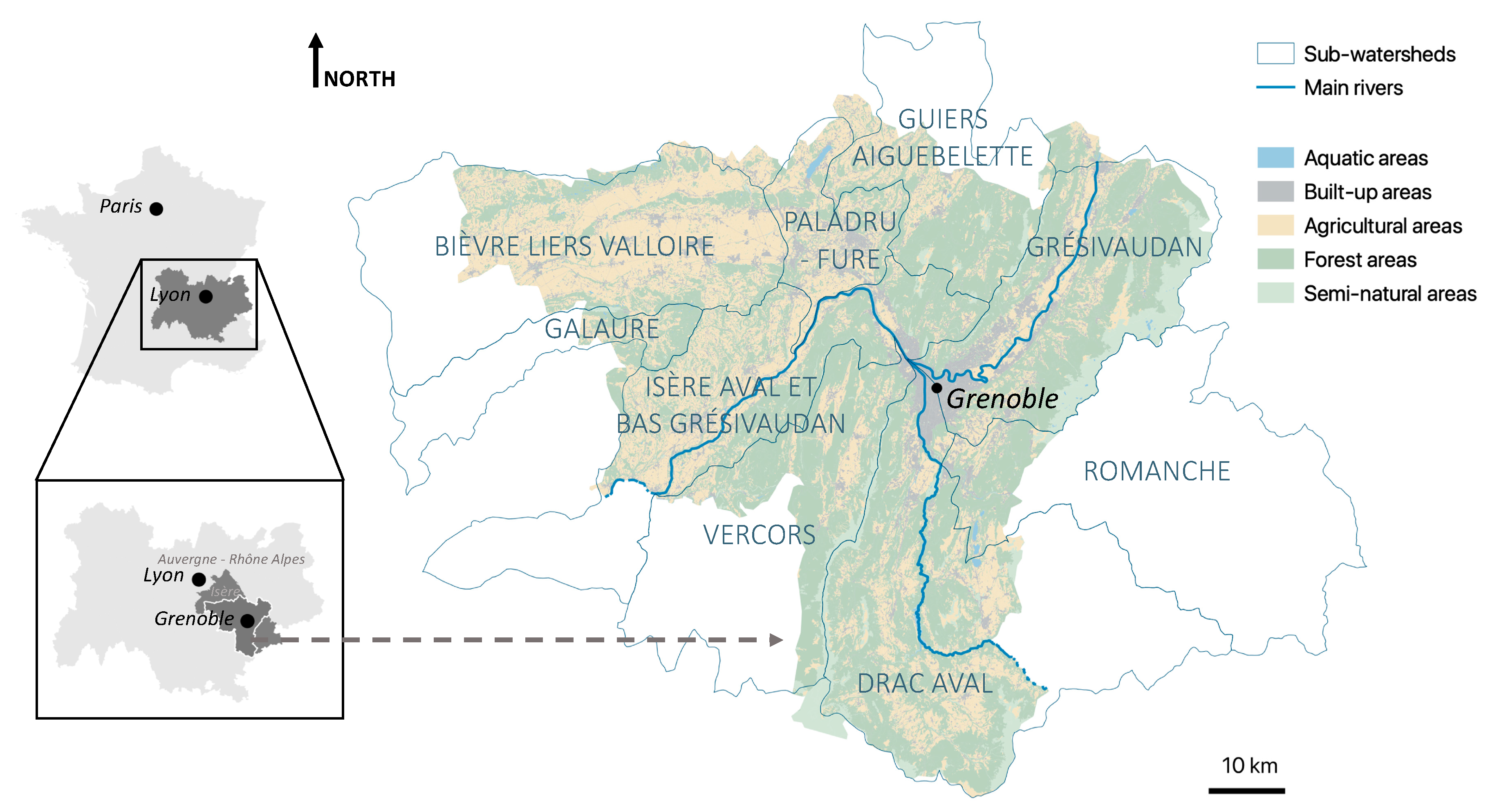
2.1. The Case Study and General Principle

Grenoble is a metropolitan area of approximately half a million people in southeastern France, at the meeting point of three Alpine valleys (Figure 1), in the Rhone and Isère river watersheds. Although the study area includes large areas of natural and seminatural habitats (forests, shrublands and woody heaths, open spaces with little or no vegetation etc.), urban sprawl and intensive agriculture occupy most of the valleys and lowlands. High-resolution Land Use and Land Cover (LULC) maps of the Grenoble region were simulated for 2009–2040 under various socioeconomic scenarios using a spatially explicit statistical model combining a GIS deterministic approach and the probabilistic platform Dinamica EGO [44,45]. Our analysis focused on the conversion of wetlands under a “business as usual” scenario, under which LULC change occurs as set out in existing zoning regulations such as the 2011 Schéma de COhérence Territorial (SCOT) [46,47]. The offsetting of the impacts of urbanization on 170 ha of wetlands was added to the model.

We used existing planning rules and recommendations to guide the location of offsets. Impacts to wetlands trigger the mitigation hierarchy in France under articles L. 211–1 and L. 212–1 of the French environmental code, with operational details laid out in watershed specific regulations such as the Schéma Directeur d’Aménagement et de Gestion des Eaux Rhône Méditerranée Corse (SDAGE RMC), in application of the European Water Framework Directive [48,49].

The definition and delimitation of wetlands in France has been the subject of much controversy in recent years, particularly in relation to the requirements they trigger in relation to development projects. Strictly speaking, wetlands are “land, whether exploited or not, usually flooded or gorged with fresh, salt or brackish water in a permanent or temporary manner; the vegetation, when it exists, is dominated by hygrophilic plants for at least part of the year” (Article L.211–1 of the Environment Code, our translation). According to this definition, a wetland can therefore be alternatively delimited according to its hydromorphic soil or to the presence of hygrophilic vegetation. A cultivated plot with a typical wetland soil profile is therefore subject to the same mitigation hierarchy requirements as a wetland that supports native wetland vegetation. These specific definitions of wetlands in France are further discussed in Gaucherand et al. [50] and Gayet et al. [51]. The wetland data we used were produced by the most recent update of the wetland atlas of Isère and the 2013 regional ‘ecological corridors’ map (Schéma régional de cohérence écologique).

We focused on wetlands located on agricultural land. This is because mountainous terrain largely constrains the potential for urban expansion and offsetting to wetlands in valleys and lowlands, where the agriculture is the dominant LULC: annual crops (cereals such as maize), perennial crops (including some vineyards and orchards, such as walnut) and some permanent grasslands. The following areas and land cover types were not considered as potential offsetting zones: (1) wetlands located in natural habitats and forests because they are in good condition overall and provide limited opportunities for ecological gain, (2) bodies of water and other aquatic habitats that are not readily restorable as wetlands, (3) wetlands in urban areas because they would probably not be accepted by regulators as offset sites due to continued pressures and unfavorable ecological contexts, and because we cannot change urban sprawl projections by Vannier et al. [44] (post-treatment of the outputs).

The general method specifically designed for this study includes three main steps described in more detail in the following subsections:

• Step 1—Identifying the offsetting need based on the planned development (map 1 in Figure 2);
• Step 2—Identifying the potential offsetting capacity (map 2 in Figure 2);

The offsetting need and the potential offsetting capacity are described both in terms of area and using an ecological condition score developed for the purposes of this analysis.

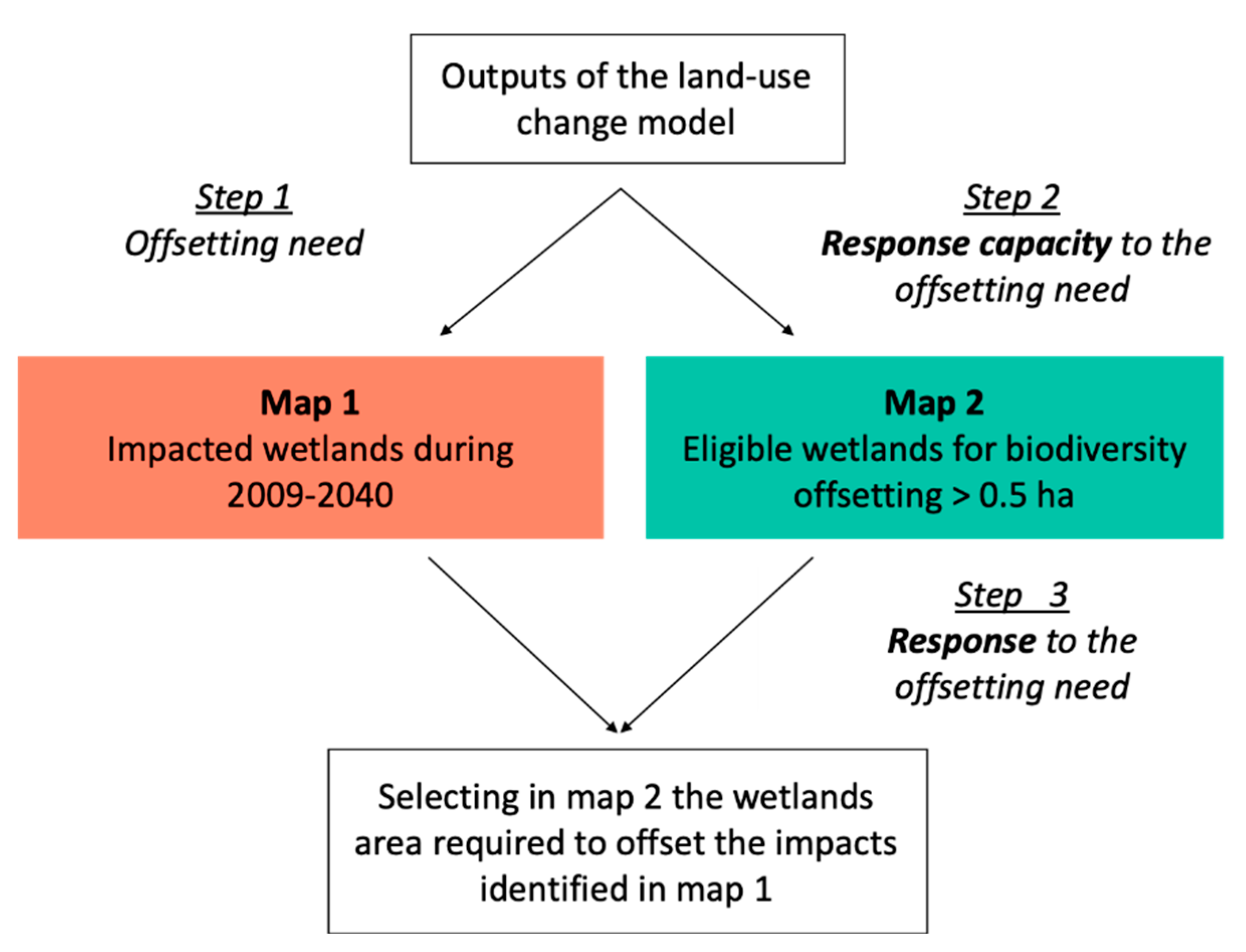
• Step 3—Modeling the offsetting response obtained: selecting in map 2 the wetland area required to offset the impacts identified in map 1, using four different biodiversity offsetting models.

2.2. Calculating the Theoretical Ecological Score for Wetlands in This Study

In order to measure variations in the ecological functions of wetlands, we determined an ecological condition score, ranging from 1 to 7/ha, based on the agricultural practices on the wetland assessed according to expert opinion (agronomists and ecologists with field experience in the study area wetlands). Vannier et al. [45] provide a detailed description of agricultural practices: 11 different classes of agricultural practices are reported at the parcel scale. Examples include “spring monocrop” or a crop rotation including “3 or 4 winter crops and a temporary grassland” [52]. The crop successions were built from the analysis of an orthophotography of the territory combined with altitudinal and climate information. A map of the major crop types (winter, spring or grassland) was produced at an annual time step between 2008 and 2012, then aggregated over 5 years, which ultimately identified the prevalent crop successions in the study area [52].. Based on the expert assessments, we proposed two different scoring systems for agricultural areas (see

Table 1. The ecological score and restoration potential scoring system.

Agricultural Practice	Ecological Score/ha Score from 1 to 7 Loss if Impacted		Ecological Restoration Potential/ha Score from 0 to 6 Gain if Restored as an Offset
Type of zone of agriculture	Intensive	Less intensive	Intensive	Less intensive
Permanent grasslands	7	7	0	0
Hedgerow	7	7	0	0
3 or 4 grasslands + 1 or 2 other land use	5	6	2	1
3 grasslands and 2 SC */3 SC et 2 grasslands	4	5	3	2
3 grasslands and 2 WC **/3 WC and 2 grasslands	4	5	3	2
2 grasslands, 2 WC, 1 other	3	4	4	3
2 grasslands, 1 SC, 1 other	3	4	4	3
Poplar	3	4	4	3
3 or 4 WC with 1 grassland	2	3	5	4
3 or 4 SC with 1 grassland	2	3	5	4
Arboriculture	2	3	5	4
SC monocropping	1	1	6	6
WC monocropping	1	1	6	6
3 or 4 SC without grassland	1	1	6	6
3 or 4 WC without grassland	1	1	6	6
3 SC and 2 WC/3 WC and 2 SC	1	1	6	6
2 WC, 2 SC, 1 other	1	1	6	6
Market gardening; horticulture	1	1	6	6
Permanent crop (orchard, wine)	1	1	6	6
Other agricultural practice	1	1	6	6

* Spring crops (SC), ** Winter crops (WC).

) linked to two altitudinal zones: intensive agriculture in lowlands and valleys, and less intensive agricultural practices in hills and mountains, mostly with livestock systems.

Wetlands that are categorized as permanent grasslands and hedgerows are generally considered to be of high environmental quality and therefore score the maximum value (7). Parcels with no grassland during a crop rotation are considered of lowest quality; however, they still trigger an offsetting need because they have some wetland features; they score the minimum value (1 not 0). These scores do not vary with the altitudinal zone. For all other agricultural practices, the higher the proportion of grassland cover in a crop rotation, the higher the ecological score. Because grasslands are much rarer in the lowland cropping systems, ecological scores for rotations with grasslands were increased to reflect their higher value in landscapes dominated by such systems (See Supplementary Material 1 for details).

We used the ecological score to assess losses and gains in wetland function and biodiversity: building on wetland leads to the loss of that area’s score, while offsetting on a wetland restores it to a maximum score of 7. The gain corresponds to the difference compared to the wetland’s initial score. No net loss is achieved if the total ecological score lost is offset by restoring an equivalent ecological score. This can be done across multiple parcels of land, with each parcel scored separately.

2.3. Three steps to Model Biodiversity Offsetting at the Landscape Scale

2.3.1. Step 1: Identifying the Offsetting Need, Map of the Impacted Wetlands

Using the development scenario outputs, we created a map of the wetlands impacted by urban expansion (map 1 of Figure 2). We selected all the urban polygons in 2040 with agricultural land in 2009 and gave them an ecological score using the scoring system described in Section 2.2. We then weighted this score according to their area to determine the total loss of wetland area and function under the planned development, for each subwatershed.

2.3.2. Step 2: Identifying Potential Offsetting Capacity, Map of the Eligible Wetlands

We then created a map of wetlands eligible for biodiversity offsetting (map 2 of Figure 2). We selected the remaining wetlands (only within agricultural land) in 2040. We removed parcels smaller than 0.5 ha that would have little chance of successful ecological restoration. In order to satisfy the additionality principle, we also removed wetlands designated as protected areas: Arrêtés de Protection de Biotope (APB), Parcs Nationaux (PN), Réserves Naturelles Nationales (RNN), Réserves Naturelles Régionales (RNR), Réserves de Biosphère (RB) of the Office National des Forêts (ONF), and areas with an existing management plan such as the Espaces Naturels Sensibles (ENS) identified by the Isère Département (see [53]). Integral reserves in the Parcs Nationaux and RAMSAR wetlands should be removed but the Grenoble area does not include any of these protected areas. We applied an ecological restoration potential score to each polygon retained using the scoring system described in Section 2.2 and weighted it by the area of the polygon to obtain the total potential ecological gain for each subwatershed.

2.3.3. Step 3: Identifying the Response to the Offset Need, Allocation Rules for Biodiversity Offsets

In order to match the impacts on wetlands identified in the first step to eligible parcels identified in the second step, in map 2 we selected as much wetland area as necessary to offset the impacts identified in map 1. We applied our approach to nine subwatersheds in the study area. The choice of offsetting wetlands was made according to the following criteria: (1) the offsetting wetlands must be located within the same subwatershed as the impacts, as required by the 2016–2021 SDAGE RMC regulations, and (2) priority is given to wetlands located within identified ecological corridors (Trames Vertes et Bleues—TVB), as suggested by current research and local government initiatives e.g., [54,55]. In addition to the above, we applied specific criteria to each of the four offsetting models (old way, local river basin plan, prospective and landscape scale) described in

Table 2. The four wetland offsetting scenarios.

Name of the Offsetting Model	Implementation Model	Ecological Equivalence Method	Type of Allocation of the Polygons *	Additional Constraint for Eligible Wetlands (Map 2)	Rationale
Old way	Permittee-led	Area based (200% area)	Automated, random	All types of parcels can be used	The way offsets have been carried out until recent changes in French policy on wetlands and mitigation hierarchy
Local river basin plan	Permittee-led	Step 1: function based (until at least 100% of the impacted area is offset)	Automated, random by decreasing ecological score To simulate the requirement to restore the most degraded wetlands (i.e., the most intensively cultivated).	Remove parcels with permanent grasslands and hedgerows Because they do not provide any ecological gain if restored, which would contradict the intention of the scenarios.	The closest to existing official local guidance and applicable regulations [56].
		Step 2: area based (until 200% of impacted area is offset)	Automated, random
Prospective	Permittee-led	Step 1: function based (100% of functions)	Automated, random by decreasing ecological score		This model is a potential improvement on current regulations and closer to other French guidelines and applicable regulations for species and other natural habitat types.
		Step 2: if area < 100%, continue with area based (until 100% of the impacted area is offset)	Automated, random
Landscape-scale	Aggregated	Function based (100% of functions) and area based (until at least 100% of impacted area is offset)	Manual, fostering high ecological restoration potential, location in ecological corridors or near a network of permanent grasslands or hedgerows, a body of water, forest or semi-natural area, not isolated in an urbanized area, contiguous parcels that would recreate ecological corridors, one single large mitigation bank rather than many small ones	All types of parcels can be used.	Similar to mitigation banking (Sites Naturels de Compensation in France) or other emerging landscape-scale approaches being developed by local governments [25].

* Shared constraints: impacts and offsets remain in the same subwatershed, priority selection of parcels located in ecological corridors when they exist.

. These include the two main challenges explored in this paper:

• Implementation models:

  ○

  an area-based method whereby a coefficient is applied to the impacted area to determine offset size, and

  ○

  a method where losses and gains of ecological function are calculated and offsets sized so as to generate enough gains to achieve functional NNL.

• Ecological equivalence methods:

  ○

  case-by-case permittee-led compensation where each developer compensates its impacts, resulting in many restored wetlands of various sizes distributed across available land, and

  ○

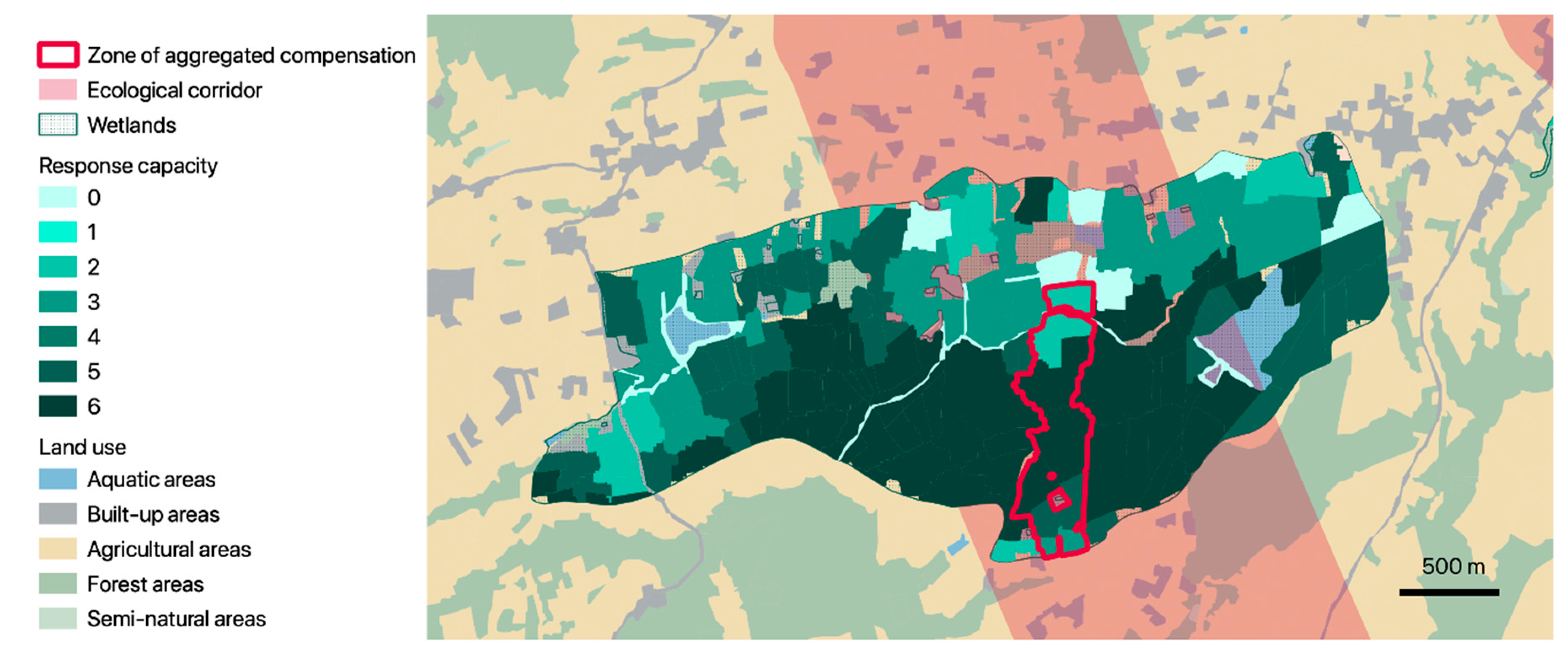
  an aggregated approach where larger sets of adjacent parcels of land are used to compensate for several projects at once, generating larger wetland units.

We used QGIS 3.10 to manage the spatial database. The allocation of offsetting parcels is the result of simulations for the first three scenarios (5000 simulations by scenario, see Box 1). The computer code is available in Supplementary Material 2 (Step 1 in the “offsetting needs” section, Step 2 in the “wetlands eligible for biodiversity offsetting” section) and Supplementary Material 3 (Step 3). The fourth scenario (landscape scale) is applied “manually” in order to model the work that would have been carried out by a mitigation banker in prioritizing wetlands for restoration and selling offset ‘credits’.

Box 1. How does the script work?

How does the script manage the preference for polygons in ecological corridors and the random selection of polygons in descending order of ecological restoration potential?

The script looks for the polygons with the highest ecological restoration potential in the subwatershed. It first selects those located in ecological corridors (if possible) and then continues with those outside of ecological corridors. When switching to the next level of ecological restoration potential, it again begins by selecting those inside the ecological corridors.

How does the script stop when the objectives are reached?

When the script selects the last polygon that exceeds the scenario objective, different procedures are applied according to the scenario. A 0.5 ha margin of error compared to area objectives is tolerated, but full compliance with the ecological score objectives is required. According to the situation, the last polygon may be kept as it is, dropped or cut to precisely fit the area or ecological score required (provided it is equal to or larger than 0.5 ha). This aspect is described in the section entitled “#Dealing with the last pick” in the computer code available in the document Supplementary Material 3.

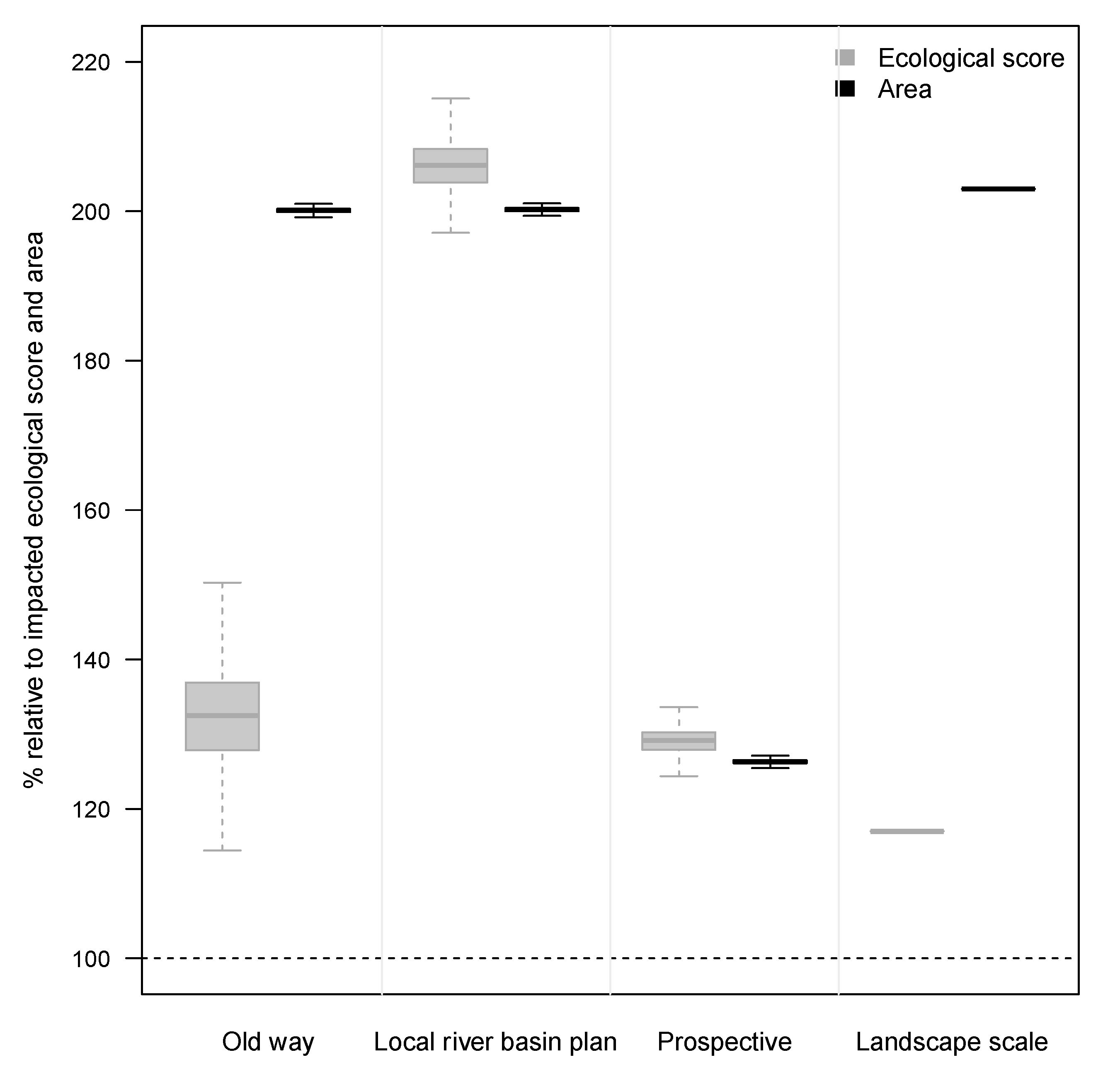
2.4. Monitored Indicators

For each offsetting scenario, we collected information on the distribution of the following indicators throughout the 5000 simulations (except for the landscape-scale scenario that was manually implemented once only):

• Area: ratio of offset area to impacted area;
• Ecological score: ratio of the restored ecological score (biodiversity offsets) to the impacted ecological score;
• Transactions: number of selected polygons that could be proxies for the number of transactions required to acquire or lease the offsetting land, and to control and monitor for regulators;
• Area for reaching NNL: area (in hectares) where 100% of the ecological score (offsetting need) is reached for the first time (for the prospective scenario only).

2.5. Supplementary Sensitivity Analyses for the Three Automated Scenarios

In addition to comparing the performance of the offsetting scenarios, we also tested two other effects. Firstly, the effect of prioritizing wetlands located in ecological corridors. Secondly, the effect of removing parcels with no grassland (those with an ecological restoration potential of 6) from the possible offsetting parcels, in order to model the potential reluctance of farmers to give up their best agricultural land to an offsetting scheme (see [57]. We did not test the effect of removing parcels with permanent grasslands and hedgerows (those with an ecological restoration potential of 0) in the old way scenario because it would contradict the aims of this area based scenario and set unlikely conditions. To conduct these supplementary analyses, we ran 5000 simulations per modified scenario.

We did not carry out supplementary tests for the landscape-scale scenario because they would set improbable conditions (in terms of eligible parcels and location prioritization) and the land tenure aspects are supposed to have been anticipated.

3. Results

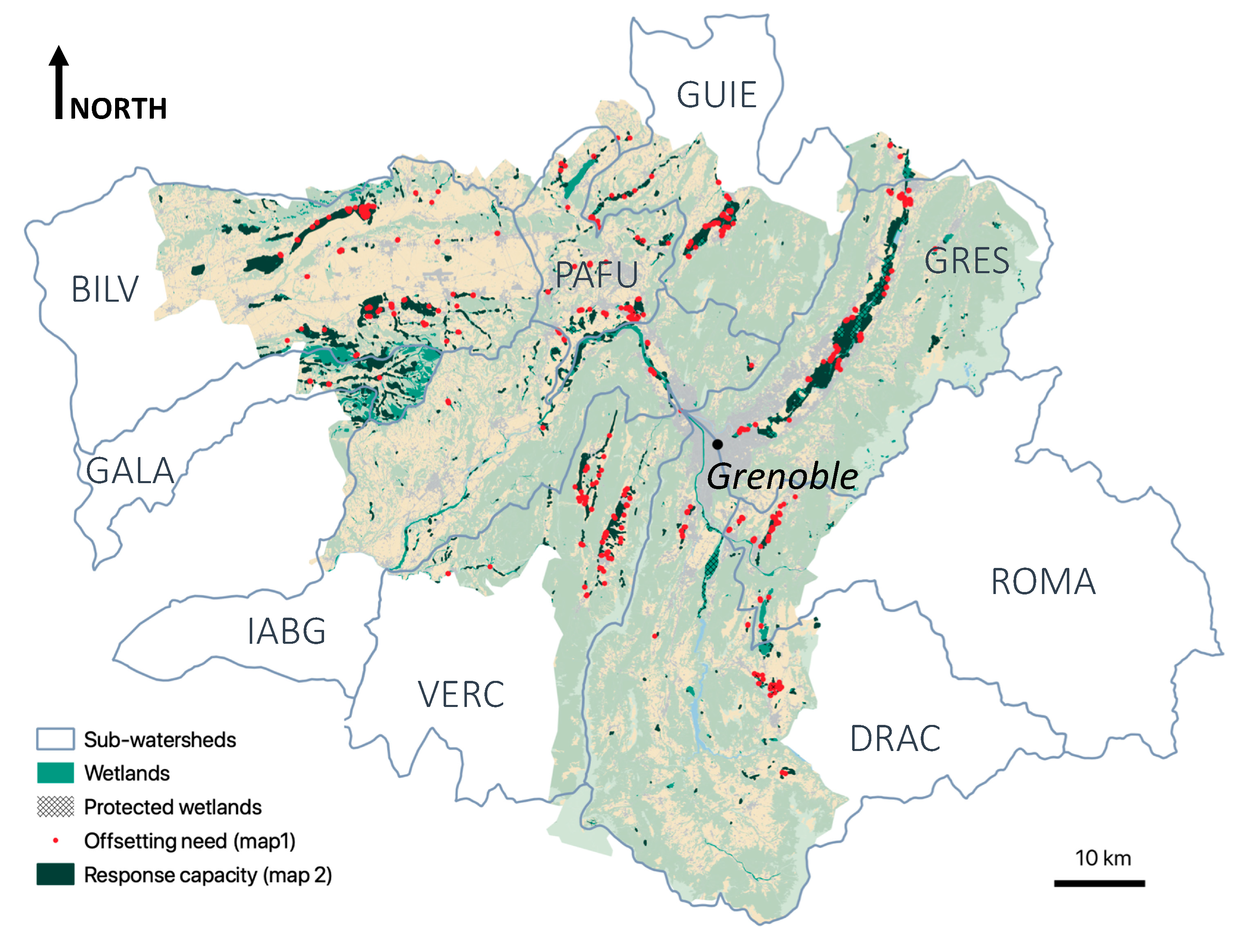
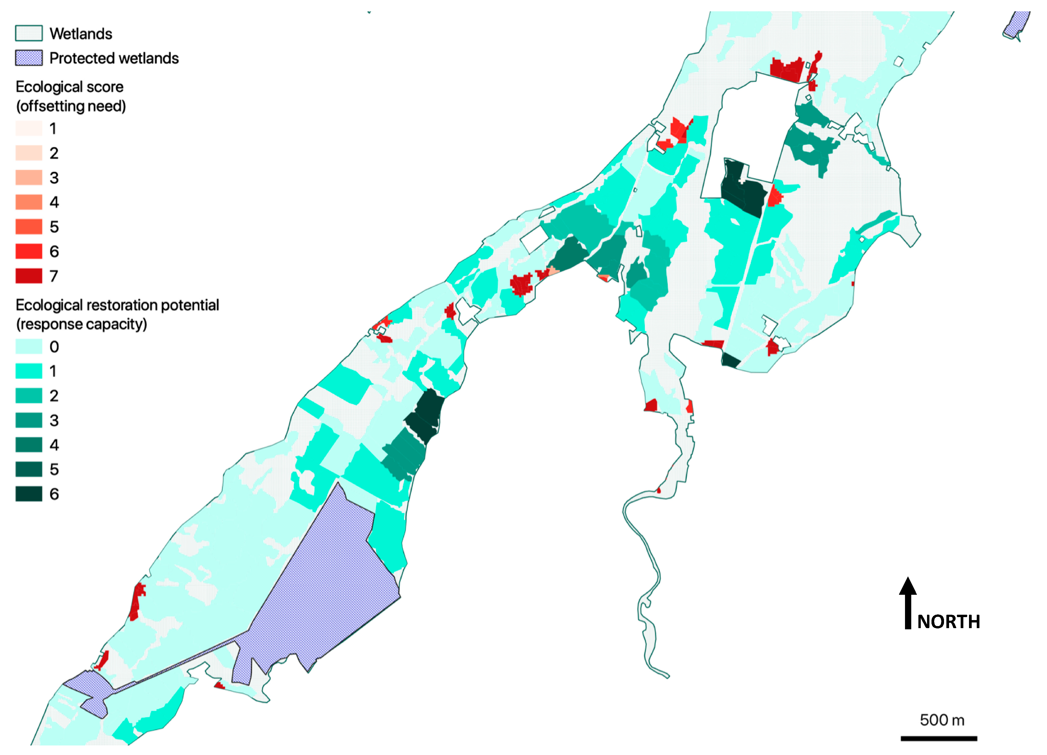
3.1. Offsetting Need and Offsetting Response Capacity (Steps 1 and 2)

In Figure 3, the red dots represent impacts on wetlands, and thus the offsetting needs (map 1). They have been magnified to make them visible at this scale.

At the study area scale (445,000 ha), 5300 ha (1.2%) are impacted by urban sprawl between 2009 and 2039, representing an 11.4% increase in built-up area (

Table 3. Evolution of the land use in the study area from 2009 to 2040.

Land Use	Area in 2009 (ha)	Evolution 2009–2040 (ha)	Evolution 2009–2040 (% of area)
Aquatic areas	4100	0	0
Built-up areas	46,800	+5300	+11.4
Agricultural areas	149,800	−6610	−4.4
Forest areas	215,600	+430	+0.2
Semi-natural areas	29,300	+138	+0.5
Fallow grounds	0	+728	N/A

). These impacts include the conversion of 170 ha of wetlands (0.7% of the wetlands in the study area), representing a loss of around 800 units of ecological score (

Table 4. Offsetting needs and potential offsetting response for wetlands, per subwatershed.

Subwatershed (Code)	Offsetting Needs		Potential Offsetting Response
	Ecological Score	Area (ha)	Ecological Score	Area (ha)
Bièvre Liers Valloire (BILV)	169	33	8910	2914
Drac aval (DRAC)	144	24	571	293
Galaure (GALA)	10	2	977	839
Grésivaudan (GRES)	83	43	8491	1786
Guiers Aiguebelette (GUIE)	159	24	448	601
Isère aval et Bas Grésivaudan (IABG)	24	5	1680	401
Paladru—Fure (PAFU)	52	12	1565	447
Romanche (ROMA)	35	11	526	131
Vercors (VERC)	114	17	173	810
TOTAL	789	170	23,343	8221

). During the same thirty-year period, the study area lost agricultural areas (−6610 ha, −4.4%), gained additional forest (+430 ha, +0.2%) and seminatural areas (+138 ha, +0.5%) and saw fallow land develop from abandoned agricultural areas (+728 ha) (Table 3).

Our analysis reveals that more than 8000 ha of wetlands (36% of the wetlands in the study area) could be eligible for biodiversity offsetting, giving an ecological restoration potential of more than 23,000 units of ecological score (Table 4). We removed around 2800 ha of wetlands designated as protected, leaving a total of 92 wetlands. The surface area of these wetlands was between 0.2 and 558 ha, with an average area of 30 ha and a median area of 8 ha (some of these wetlands are actually made up of non-adjacent parcels within a protected area).

Subwatersheds differ greatly in terms of area and total ecological scores for impacted wetlands and for potential wetlands for offsetting. For instance, the ecological score per hectare of impacted wetlands is higher in VERC than in BILV, while the opposite is true for the ecological score per potential wetland for offsetting. Moreover, while BILV and VERC have a similar impacted ecological score, the response capacity in terms of ecological score is much higher for BILV than for VERC. It is therefore necessary to express the results, both in terms of area and ecological score, using ratios to take into account the diverse situations across the subwatersheds.

The map in Figure 4 summarizes one example of offsetting needs and response capacity for an example zone within the study area.

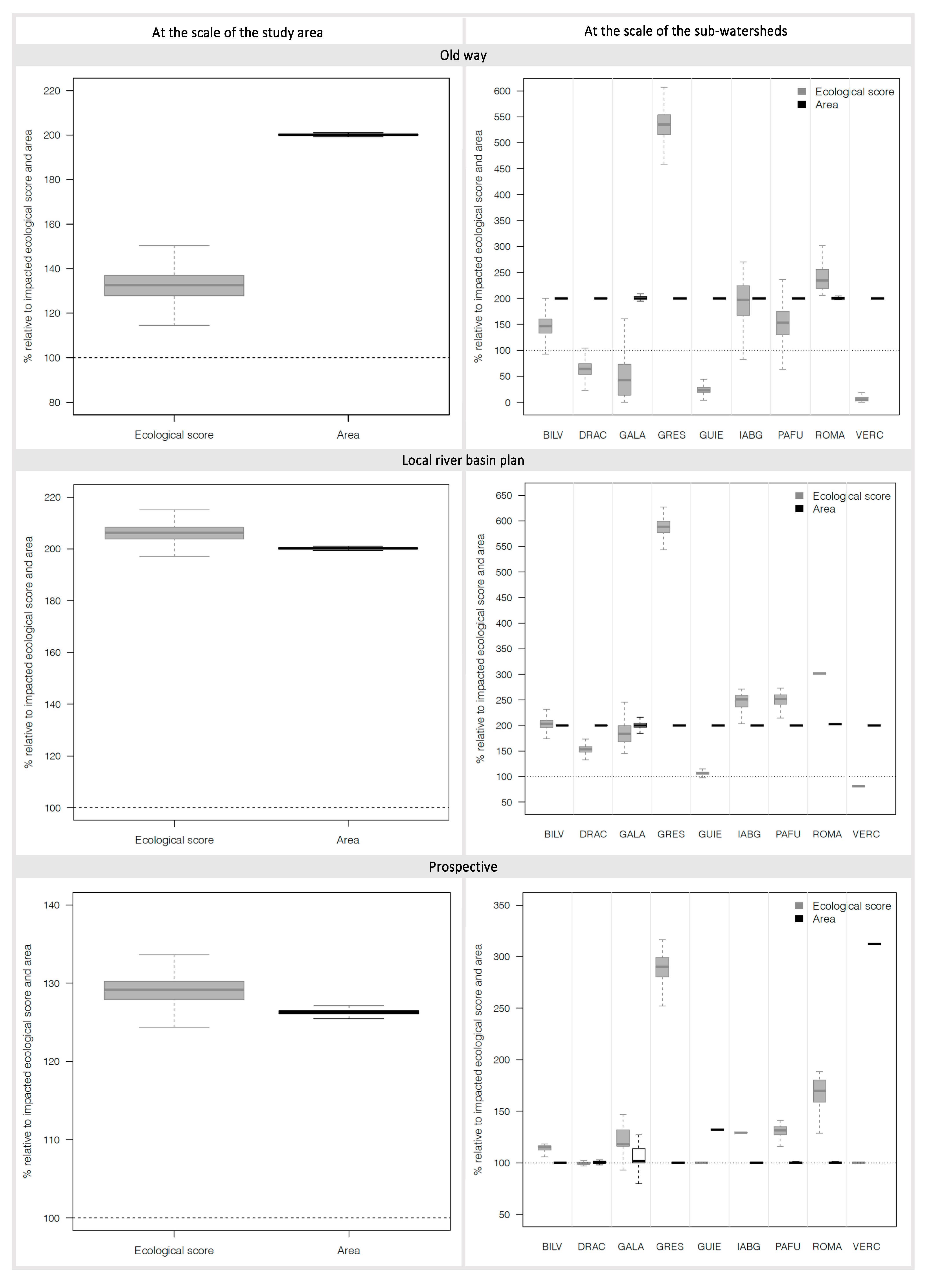
3.2. Results of the Modeling of Wetland Offsetting Scenarios (Step 3)

A general overview of the results (

Table 5. Comparison of the results at the study area scale, with ranges at subwatershed scale where applicable * for the four scenarios.

	Old Way	Local River Basin Plan	Prospective	Landscape-Scale
Area
Targeted area (% of impacted area = 170 ha)	200%	200%	<100%	<100%
Area of compensation (ha)	340 [4; 87]	340 [4; 87]	215 [2; 54]	346
Area of compensation (% of impacted area)	200% [200%; 201%]	200% [200%; 203%]	126% [100%; 312%]	203%
Area of compensation (% of the response capacity in area)	4.1% [0.4%; 16.3%]	4.1% [0.4%; 16.4%]	2.6% [0.2%; 8.2%]	4.1%
Ecological score
Targeted ecological score (% of impacted ecological score = 800)	-	-	100%	100%
Ecological score of compensation (ecological score)	1 045 [4; 444]	1 630 [18; 488]	1 020 [11; 240]	926
Ecological score of compensation (% of impacted ecological score)	132% [6%; 534%]	206% [82%; 587%]	129% [100%; 289%]	117%
Ecological score of compensation (% of the response capacity in ecological score)	4.5% [0.4%; 16.3%]	7% [1.8%; 53.6%]	4.4% [1.2%; 65.7%]	3.9%
Transactions
Number of parcels	175	166	108	150 (16 groups)

* shown in square brackets: range of values at the subwatershed scale.

, Figure 5) shows that each scenario was feasible and achieved its set objectives. The compensation area only requires a small proportion of the potential offsetting capacity (with considerable excess wetlands available in some subwatersheds). The ecological gain from offsetting represents a small proportion of the total potential restoration capacity (less than 10%), but in some subwatersheds, more than 50% of the potential response capacity is required to implement the local river basin plan and prospective offsetting scenarios. Figure 6 details the results for the automated scenarios at the subwatershed scale.

Under the old way scenario, when 200% of the impacted area is targeted (340 ha), the resulting ecological gain is 132% (1045 ecological score) of the loss at the study area scale (Table 5). However, at the subwatershed scale, four of the nine subwatersheds obtained an ecological gain of less than 100% and hence a net loss of wetland function and biodiversity (Figure 6). Our theoretical results show that this old way scenario achieves NNL of biodiversity overall, but this conceals situations of net biodiversity loss in nearly half of the region’s subwatersheds.

Under the local river basin plan scenario, when 200% of the impacted area is targeted (340 ha) with the constraint of choosing the offsetting parcels with the best ecological restoration potential for at least 100% of the impacted area, the resulting ecological gain is 206% (1630 score) of the loss, at the study area scale (Table 5). Compared to the old way scenario, it requires more overall surface area, but only one subwatershed (Vercors) fails to achieve NNL (Figure 6).

Under the prospective scenario, when NNL of ecological score and at least 100% of impacted area is targeted (170 ha), with the constraint of choosing parcels with the best ecological restoration potential, the resulting ecological gain is 129% (1020 score) of the loss, across the entire study area (Table 5). Compared to the first two scenarios, only 126% of the impacted area is enough to ensure the offsetting of an area equivalent to 100% of impacted area, as well as NNL of wetland function and biodiversity, which is achieved in all the subwatersheds (Figure 6).

Table 6. Area required to reach NNL.

Subwatershed (CODE)	Offsetting Area for Reaching NNL of Wetland Function and Biodiversity	Offsetting Area Required to Achieve Both NNL and An Area at Least Equal to the Area Impacted
	(% of Impacted Area, Mean Value for the 5000 Simulations)
Bièvre Liers Valloire (BILV)	93%	100%
Drac aval (DRAC)	101%	101%
Galaure (GALA)	104%	104%
Grésivaudan (GRES)	37%	100%
Guiers Aiguebelette (GUIE)	132%	132%
Isère aval et Bas Grésivaudan (IABG)	95%	100%
Paladru—Fure (PAFU)	88%	100%
Romanche (ROMA)	71%	100%
Vercors (VERC)	312%	312%
All the subwatersheds	106%	126%

shows that, on average, 106% of the impacted area would be enough to obtain NNL. Five of the nine subwatersheds reach NNL with an offset area of less than 100% of the impacted area, but in some cases, a much greater surface area is needed. For instance, while 37% of the impacted area is enough to offset the loss of ecological score in the GRES subwatershed, 312 is required for the VERC subwatershed.

The landscape-scale scenario achieves the desired objective (117% of the NNL target) with 16 mitigation banks covering a total of 346 ha, corresponding to 203% of the impacted area (

Table 7. Results in terms of area and ecological score per subwatershed and at the study area scale for the landscape-scale offsetting scenario.

Subwatershed (Code)	Result Relative to the Objective (Ecological Score)	Result Relative to the Objective (Area)	Number of Mitigation Banks	Size of the Mitigation Banks (ha)
Bièvre Liers Valloire (BILV)	103%	112%	1	37
Drac aval (DRAC)	104%	180%	3	29, 10, 4
Galaure (GALA)	101%	226%	1	4
Grésivaudan (GRES)	236%	105%	1	45
Guiers Aiguebelette (GUIE)	102%	377%	2	52, 37
Isère aval et Bas Grésivaudan (IABG)	101%	108%	1	6
Paladru—Fure (PAFU)	115%	120%	1	14
Romanche (ROMA)	102%	113%	1	12
Vercors (VERC)	100%	557%	5	35, 25, 24, 8, 4
TOTAL	117%	203%	16	346

). The need for a larger area than the impacted area is, in part, due to the fact that for some subwatersheds, selecting parcels with the highest ecological restoration potential would have led to an overshoot in terms of wetland function gains. Figure 7 illustrates this landscape-scale scenario with a 37 ha mitigation bank in one of the subwatersheds which reconnects previously fragmented wetlands within an ecological corridor.

The smallest mitigation banks cover 4 ha and the largest 52 ha, with a median value of approximately 20 ha. These values are lower than the 100 ha minimum proposed by Moreno-Mateos et al. [58] for successful wetland restoration, but they are consistent with the mean and median size of protected wetlands in the study area, albeit smaller. One can conclude that in our case study area, the offsetting need per subwatershed is too low to establish wetland mitigation banks that are large enough to be effective. One alternative could be a single mitigation bank covering the offsetting needs of the whole study area. This is indeed achievable, with contiguous parcels covering 170 ha, generating an ecological gain of 800 (ecological score) if restored. Although such a bank could potentially address the loss of biodiversity, it would largely ignore other lost local ecological functions such as flood regulation which are more relevant within a subwatershed. A more suitable option would be to embed mitigation banks into broader wetland restoration programs with blended funding mechanisms. Such as approaches have been developed around Chambéry (another Alpine city) and are discussed in Quétier et al. [55] and Vaissière and Meinard [59].

The number of potential transactions is slightly lower for the prospective (108) scenario compared to the other three offsetting scenarios (mean of 166 parcels). This can be explained by the fact that this scenario optimizes the number of hectares (prioritization of the parcels with the highest ecological restoration potential) needed to reach NNL in terms of ecological score. It does not systematically target 200% of the impacted area like the old way and local river basin plan scenarios. By design, the number of transactions is the lowest for the landscape-scale scenario for which 150 parcels would need to be acquired, leased or at least pre-identified to form 16 groups of parcels to be managed as units. This makes it the simplest scenario in terms of regulatory control and monitoring.

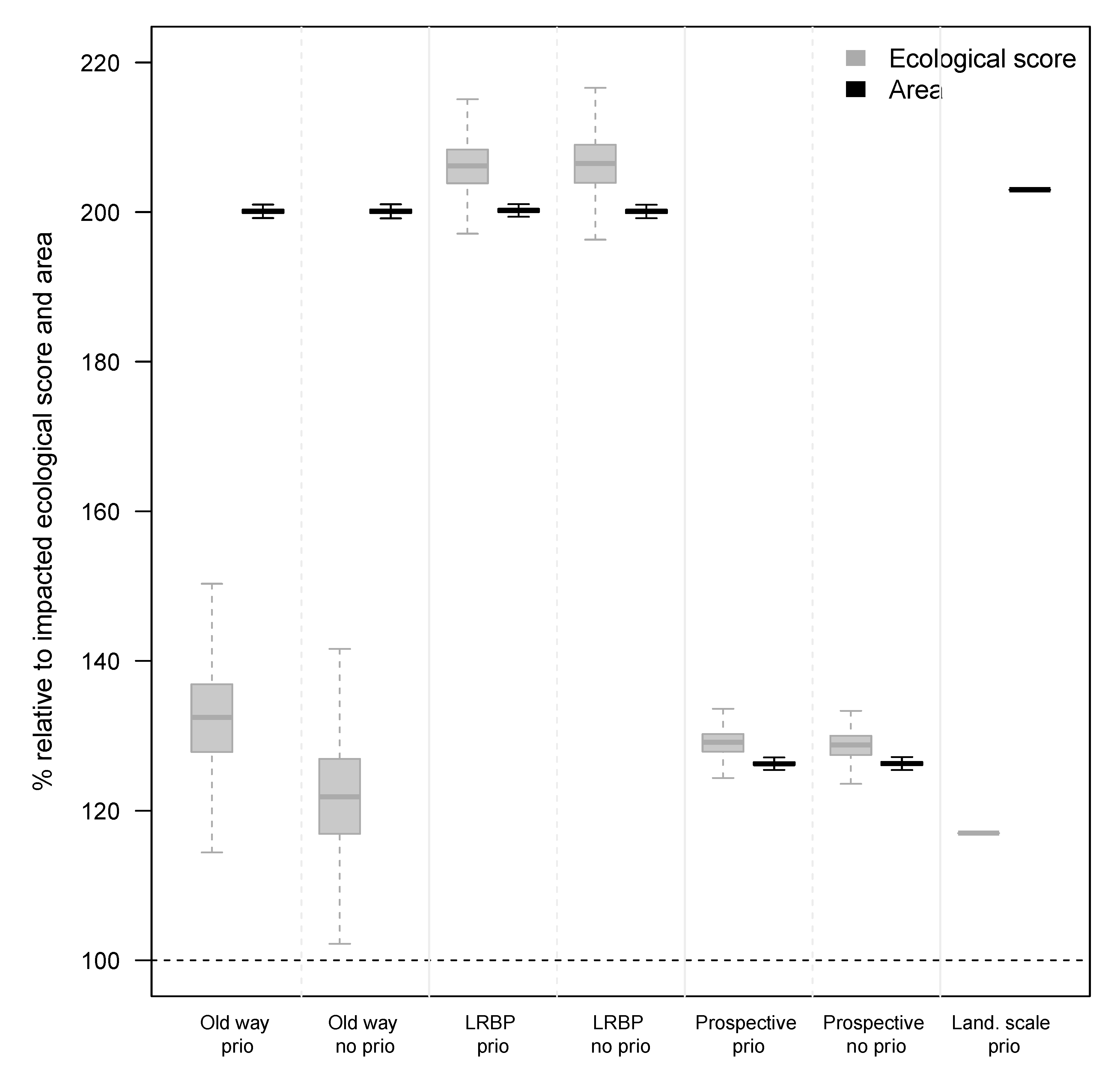
3.3. Results of the Supplementary Sensitivity Analyses

3.3.1. Effect of Prioritizing Wetlands Located in Ecological Corridors

Constraining the location of offsets to ecological corridors does not dramatically change the results of the three automated scenarios except for the old way scenario, under which additional ecological gains are achieved through this prioritization (Figure 8). However, our modeling does not reward the other likely ecological benefits obtained by improving the conservation status and functionality of corridors.

3.3.2. Effect of Removing Parcels with No Grassland from the Possible Offsetting Parcels

Taking into account the potential reluctance of farmers to sell or lease their best land diminishes the performance of the three automated offsetting scenarios (Figure 9). This was expected because the polygons with the best ecological score are removed from the pool of available offsetting land. The old way scenario even shifts to a global net loss, as one would expect under an averted-loss offsetting system.

Regarding the prospective scenario, when the best agricultural parcels were available, 126% of the impacted area was required to reach 129% in terms of ecological score (106% of the impacted area to reach at least NNL of biodiversity,

Table 8. Comparison of the area required to reach NNL under the prospective scenario and with the supplementary analysis.

Subwatershed (CODE)	Area for Reaching NNL (% of Impacted Area, Mean Value for the 5000 Simulations)
	Prospective Scenario	Prospective Scenario without the Best Agricultural Parcels
Bièvre Liers Valloire (BILV)	93%	102%
Drac aval (DRAC)	101%	147%
Galaure (GALA)	104%	104%
Grésivaudan (GRES)	37%	44%
Guiers Aiguebelette (GUIE)	132%	193%
Isère aval et Bas Grésivaudan (IABG)	95%	100%
Paladru—Fure (PAFU)	88%	98%
Romanche (ROMA)	71%	94%
Vercors (VERC)	312%	500%
All the subwatersheds	106%	146%

). When the best parcels are removed under the prospective scenario, 161% of the impacted area is required to achieve an ecological gain of 116%, compared to 126% and 129%, respectively, when the best agricultural land is available. To reach NNL in terms of ecological score, excluding the best land increases the area required from 106% to 146% of the impacted area (Table 8). These differences hit peaks of 500% for the VERC subwatershed. Only the GRES subwatershed produces results anywhere near this figure in the other three scenarios (Supplementary Material 4). To conclude, when the best agricultural parcels are removed, along with the highest potential for ecological gain, much more land is required to achieve NNL.

The full results for the three automated scenarios and the supplementary analyses (at the study and subwatershed scales) can be found in Supplementary Material 4.

4. Discussion

4.1. Lessons Learned Regarding the Performance of Offsetting Approaches

The old way scenario leads to NNL of ecological function and biodiversity at the scale of the whole case study landscape, but this conceals local net loss outcomes. This reflects the limits of the area-based approaches to offsetting that were widely used for many years in France, and still are in many countries [1]. Taking into account the likely reluctance of farmers to give up their best farmland for wetland restoration exacerbates this risk, leading to an overall net loss. However, this reluctance has been repeatedly highlighted, e.g., [57,60,61]. Although at present it is not common practice, prioritizing offsets in ecological corridors improves the ecological quality of offsetting

More recent practices based on functional approaches, as modeled in the local river basin plan and prospective scenario, perform better. NNL is achieved overall and in almost all subwatersheds under the local river basin plan scenario, even if no specific objectives are given in terms of ecological score. This is reassuring because it shows that the current local public policy in place will help achieve NNL more consistently than past practices. By design, the prospective scenario leads to NNL of wetland function and biodiversity at all scales, with a lower area requirement (and a lower net ecological score) than the local river basin plan scenario. This demonstrates that NNL can be achieved using less land for offsetting (while nevertheless aiming to offset at least 100% of the impacted area) and hence at a lower cost. This is consistent with recent changes in French government guidance and regulations which, since 2016, have shifted their focus towards measurable ecological outcomes from mitigation hierarchy.

Under the landscape-scale scenario, aggregated offsets also achieve NNL, but more land is needed due to the constraints of restoring neighboring parcels. Aggregated offsets are recommended more and more often and are used worldwide to achieve longer-lasting biodiversity gains from more ambitious and larger-scale restoration projects, and to enable the implementation of more robust governance, as it is much easier to monitor and enforce a smaller number of offset sites. However, these organizational benefits of a smaller number of larger management units are not directly apparent when comparing the ecological performance of the modeled scenarios. The reluctance of farmers to sell or lease their best agricultural land could, however, be more easily addressed in this scenario under which land can be secured in advance.

4.2. Cost-Effectiveness Implications

Overall, ignoring the organizational limitations of permittee-led approaches, which have been shown to be ineffective and costly [6,48], can mask the risk of offsets that are never actually implemented. The ecological performance of the corresponding scenarios may therefore be overestimated. Their economic performance also matters, and our analyses show that to achieve NNL, the most effective approach is to implement urban development projects on land which is used for intensive agriculture and to select the same type of land for offsetting to obtain the highest gains per unit area (more intensively used land has higher restoration potential). However, the cost of obtaining such land could be a barrier to implementation. Ecological restoration of larger areas of less intensively used, and therefore cheaper, farmland may be more cost-effective. Large land takes for ecological restoration go against other public policies aimed at maintaining agricultural potential, which developers may ignore when looking for the most cost-effective way to comply with NNL requirements. More costly offsets might also promote avoidance (less sprawl) and thereby densification, and brownfield over greenfield projects.

4.3. Wetland Condition Scoring and Its Limitations

The ecological scores used to assess losses and gains are imperfect proxies for the multiple values and functions of wetlands, and are biased towards wetland biodiversity.

Although our knowledge of agricultural practices is quite advanced and detailed compared to previous studies (e.g., our scoring is done at the parcel scale and takes crop rotation into consideration), some important criteria were not taken into account, such as the location of the parcel relative to other ecological features or environmentally friendly practices such as organic agriculture (no pesticides). Moreover, permanent grasslands might vary in their ecological condition depending on drainage, fertilization or species mix. Similarly, the value of poplar plantations may depend on the presence and characteristics of a herbaceous substratum. More generally speaking, although we do not have this information, there are many different types of wetlands and they are not all substitutable. However, as our models require the offsets to be located in the same subwatershed as the impacts this should limit these types of substitutions.

Several ecological functions of wetlands, such as their hydrological or biogeochemical functions, were not explicitly considered in the scoring system. Additional spatial information sources could be used to take into account the benefits of fully functional wetlands such as soil roughness (e.g., through Corine Land Cover), wetland slopes and proximity to hydrological network, but this would require complementary field investigations. Considering the dominant fertilizers and pesticide treatments, or tillage techniques, associated with each crop rotation could have provided a more nuanced scoring of such functions.

In practice, the assessment of wetland condition for mitigation and offsetting purposes tends to be based on vegetation, which lends credit to our approach. One such example is the MERCIe method by Mechin and Pioch [62], but many different scoring methods have been developed by consultancies. A national method was developed [51,63] with a view to obtaining a uniform approach. Under this method, scores are based on the calculation of a number of indicators (produced from spatial and field data) with a scientifically proven link to hydrological, biogeochemical and biological functions. The analysis of loss and gain is only produced indicator-by-indicator (no overall score) and makes it possible to take into account the overall functionality of wetlands when establishing NNL, rather than their biodiversity value alone.

It is also important to note that the uncertainties and time-lags associated with restoration potential were ignored when assessing scenario performance. In an improved version of the modeling, an uncertainty factor could be applied as a correction factor to areas of less than 100 ha or 30 ha, and/or through a bonus when these minimum area thresholds are reached, to reflect the likely increased restoration potential of larger wetlands. Such corrections would have increased the relative performance of the landscape-scale scenario. Other determinants of wetland restoration potential could also be included, if available, such as information on time-lags which can be lengthy when restoring peatlands or forested wetlands. In our modeling, we assumed that all restoration would be effective by 2040. An improved version of our modeling might look at performance over time (e.g., annual steps as in [33]), and at the exact timing of impact—offset exchanges, which Gordon et al. [37], among others, have shown is critical to the overall outcome. Our modeling also ignores the potential for some wetlands to increase their ecological score through natural (spontaneous) restoration, thereby overestimating offset gains.

Ecological outcomes may have also been underestimated by ignoring the ecological benefits of locating offsets in ecological corridors in need of restoration or reconnection. This could be rewarded in an improved version of the modeling with a bonus added if a polygon contributes to restoring an ecological corridor or if contiguous selected polygons create a path throughout an identified ecological corridor (as illustrated in Figure 7). The potential contribution of offsets to the restoration of landscape-scale ecological processes has been highlighted recently [41,54,64].

We focused on wetlands in a mountain landscape (Alpine biogeographical region). Applying our modeling approach to other types of biodiversity is not without challenges. While most offsets in France are triggered by impacts to protected species, a uniform scoring system would be irrelevant for endangered species [48]. The NNL goal is particularly complicated to describe and achieve for endangered species, for which available data is often patchy compared to habitats such as wetlands. Habitat or ecosystem-based approaches, however, are useful for obtaining umbrella metrics for numerous species and other ecological features [61].

4.4. Practical Applications: Assessing a Region’s Development Carrying Capacity

One practical application of our modeling approach is that it enables decision makers to compare offsetting scenarios and determine if, and how, a development decision or pathway/scenario can be made compatible with a NNL goal. This ‘carrying capacity’ can serve as the basis for feasibility studies for local development programs and should help anticipate potential situations of ‘saturation’ where there are no further offsetting options available. In our case study, all the scenarios require a small part of the area’s available wetlands for offsetting, in most of the subwatersheds. Compared to previous studies, we have focused on a rather small area (4450 km² and ~800,000 inhabitants), but this corresponds to the administrative level at which decisions on development and offsetting are actually made. Conducting the same analysis in other French contexts (e.g., with higher rates of urban expansion, less avoidance or more limited offsetting opportunities) could produce more dramatic results. In their analysis of Australia, Brazil, Indonesia and Mozambique, Sonter et al. [33] describe situations where there is not enough land available to respond to the biodiversity offsetting requirements triggered by development. The data needed for such analyses (high quality land use information), however, is only rarely available, which limits the scope of use of our approach.

In addition, our modeling approach is not a turnkey solution for selecting parcels for offsetting measures. There is a need for field analysis, when the final decision is made at the local level, in order to assess the current ecological quality of the parcels to be developed and the ecological restoration potentiality of compensation sites.

What happens if it is shown that the development carrying capacity of an area will be exceeded? Is the NNL goal unattainable? As our results show, part of the answer to this question lies in the scale at which NNL is to be achieved (e.g., the whole landscape or subwatersheds?). The point in time when NNL is achieved also matters, although we did not explicitly investigate this. Rather than trying to impose blanket NNL requirements, it makes more sense to first set conservation and restoration targets in time and space. Building on the suggestion by Simmonds et al. [17] to design and implement offsets so as to contribute to achieving such biodiversity targets, Vaissière and Meinard [59] suggested embedding biodiversity offsets into conservation programs. As such, offsetting is only one lever for a wider ambition that is easier to explain to project proponents and elected officials than the “quest for ecological neutrality”. The latter, in its current form, is not widely accepted and generally appears to be an inappropriate and technocratic goal, unable to withstand the pressure of development needs.

References

1. Ermgassen, Z.S.O.; Baker, J.; Griffiths, R.A.; Strange, N.; Struebig, M.J.; Bull, J.W. The ecological outcomes of biodiversity offsets under “no net loss” policies: A global review. Conserv. Lett. 2019, 12, e12664. [Google Scholar] [CrossRef] [Green Version]
2. Bull, J.W.; Lloyd, S.P.; Strange, N. Implementation gap between the theory and practice of biodiversity offset multipliers. Conserv. Lett. 2017, 10, 656–669. [Google Scholar] [CrossRef]
3. Wende, W.; Tucker, G.; Quétier, F.; Rayment, M.; Darbi, M. (Eds.) Biodiversity Offsets—European Perspectives on No Net Loss of Biodiversity and Ecosystem Services; Springer: Cham, Germany, 2018; ISBN 9783319725796. [Google Scholar]
4. Bas, A.; Imbert, I.; Clermont, S.; Reinert, M.E.; Calvet, C.; Vaissière, A.C. Approches anticipées et planifiées de la compensation écologique en Allemagne: Vers un retour d’expérience pour la France? Sci. Eaux Territ. 2020, 31, 44–49. [Google Scholar]
5. Schoukens, H. Habitat Restoration Measures as Facilitators for Economic Development within the Context of the EU Habitats Directive: Balancing No Net Loss with the Preventive Approach? J. Environ. Law 2017, 29, 47–73. [Google Scholar] [CrossRef]
6. Weissgerber, M.; Roturier, S.; Julliard, R.; Guillet, F. Biodiversity offsetting: Certainty of the net loss but uncertainty of the net gain. Biol. Conserv. 2019, 237, 200–208. [Google Scholar] [CrossRef]
7. Tucker, G.M.; Quétier, F.; Wende, W. Guidance on Achieving No Net Loss or Net Gain of Biodiversity and Ecosystem Services; Report to the European Commission; DG Environnement on Contract ENV.B.2/SER/2016/0018; IEEP: Brussels, Belgium, 2020. [Google Scholar]
8. Bull, J.W.; Suttle, K.B.; Gordon, A.; Singh, N.J.; Milner-Gulland, E.J. Biodiversity offsets in theory and practice. Oryx 2013, 47, 369–380. [Google Scholar] [CrossRef] [Green Version]
9. Walker, S.; Brower, A.L.; Stephens, R.T.; Lee, W.G. Why bartering biodiversity fails. Conserv. Lett. 2009, 2, 149–157, in press. [Google Scholar] [CrossRef]
10. Gardner, T.A.; Von Hase, A.; Brownlie, S.; Ekstrom, J.M.; Pilgrim, J.D.; Savy, C.E.; Stephens, R.T.; Treweek, J.O.; Ussher, G.T.; Ward, G.; et al. Biodiversity offsets and the challenge of achieving no net loss. Conserv. Biol. 2013, 27, 1254–1264. [Google Scholar] [CrossRef]
11. McKenney, B.A.; Kiesecker, J.M. Policy development for biodiversity offsets: A review of offset frameworks. Environ. Manag. 2010, 45, 165–176. [Google Scholar] [CrossRef]
12. BenDor, T.; Brozović, N. Determinants of spatial and temporal patterns in compensatory wetland mitigation. Environ. Manag. 2007, 40, 349–364. [Google Scholar] [CrossRef]
13. Bezombes, L.; Regnery, B. Séquence Éviter-Réduire-Compenser: Des enjeux écologiques aux considérations pratiques pour atteindre l’objectif d’absence de perte nette de biodiversité. Ingénieries 2020, 31, 4–9. [Google Scholar]
14. Bigard, C.; Thiriet, P.; Pioch, S.; Thompson, J.D. Strategic landscape-scale planning to improve mitigation hierarchy implementation: An empirical case study in Mediterranean France. Land Use Policy 2020, 90, 104286. [Google Scholar] [CrossRef]
15. Grimm, M.; Köppel, J.; Geißler, G. A Shift towards Landscape-Scale Approaches in Compensation-Suitable Mechanisms and Open Questions. Impact Assess. Proj. Apprais. 2019, 37, 491–502. [Google Scholar] [CrossRef]
16. Kiesecker, J.M.; Copeland, H.; Pocewicz, A.; McKenney, B. Development by design: Blending landscape-level planning with the mitigation hierarchy. Front. Ecol. Environ. 2010, 8, 261–266. [Google Scholar] [CrossRef]
17. Simmonds, J.S.; Sonter, L.J.; Watson, J.E.M.; Bennun, L.; Costa, H.M.; Edwards, S.; Grantham, H.; Griffiths, V.F.; Jones, J.P.G.; Kiesecker, J.; et al. Moving from biodiversity offsets to a target-based approach for ecological compensation. Conserv. Lett. 2020, 12, e12695. [Google Scholar] [CrossRef] [Green Version]
18. Underwood, J.G. Combining landscape-level conservation planning and biodiversity offset programs: A case study. Environ. Manag. 2011, 47, 121–129. [Google Scholar] [CrossRef] [PubMed]
19. Bennett, G.; Gallant, M.; Ten Kate, K. State of Biodiversity Mitigation 2017: Markets and Compensation for Global Infrastructure Development; Forest Trends’ Ecosystem Marketplace: Washington, DC, USA, 2017. [Google Scholar]
20. Vaissière, A.C.; Levrel, H. Biodiversity offset markets: What are they really? An empirical approach to wetland mitigation banking. Ecol. Econ. 2015, 110, 81–88. [Google Scholar] [CrossRef] [Green Version]
21. Poudel, J.; Zhang, D.; Simon, B. Estimating the demand and supply of conservation banking markets in the United States. Land Use Policy 2018, 79, 320–325. [Google Scholar] [CrossRef]
22. Poudel, J.; Zhang, D.; Simon, B. Habitat conservation banking trends in the United States. Biodivers. Conserv. 2019, 28, 1629–1646. [Google Scholar] [CrossRef]
23. Grimm, M. Conserving biodiversity through offsets? Findings from an empirical study on conservation banking. J. Nat. Conserv. 2020, 57, 125871. [Google Scholar] [CrossRef]
24. Kleining, B. Biodiversity protection under the habitats directive: Is habitats banking our new hope? Environ. Law Rev. 2017, 19, 113–125. [Google Scholar] [CrossRef]
25. Ollivier, C.; Spiegelberger, T.; Gaucherand, S. La territorialisation de la séquence ERC: Quels enjeux liés au changement d’échelle spatiale? Sci. Eaux Territ. 2020, 1, 50–55. [Google Scholar] [CrossRef]
26. Tulloch, A.I.; Gordon, A.; Runge, C.A.; Rhodes, J.R. Integrating spatially realistic infrastructure impacts into conservation planning to inform strategic environmental assessment. Conserv. Lett. 2019, 12, e12648. [Google Scholar] [CrossRef] [Green Version]
27. Whitehead, A.L.; Kujala, H.; Wintle, B.A. Dealing with cumulative biodiversity impacts in strategic environmental assessment: A new frontier for conservation planning. Conserv. Lett. 2017, 10, 195–204. [Google Scholar] [CrossRef]
28. Moilanen, A.; Van Teeffelen, A.J.; Ben-Haim, Y.; Ferrier, S. How much compensation is enough? A framework for incorporating uncertainty and time discounting when calculating offset ratios for impacted habitat. Restor. Ecol. 2009, 17, 470–478. [Google Scholar] [CrossRef]
29. Cole, S.G. Wind power compensation is not for the birds: An opinion from an environmental economist. Restor. Ecol. 2011, 19, 147–153. [Google Scholar] [CrossRef] [Green Version]
30. Quétier, F.; Lavorel, S. Assessing ecological equivalence in biodiversity offset schemes: Key issues and solutions. Biol. Conserv. 2011, 144, 2991–2999. [Google Scholar] [CrossRef]
31. Laitila, J.; Moilanen, A.; Pouzols, F.M. A method for calculating minimum biodiversity offset multipliers accounting for time discounting, additionality and permanence. Methods Ecol. Evol. 2014, 5, 1247–1254. [Google Scholar] [CrossRef] [Green Version]
32. Marshall, E.; Wintle, B.A.; Southwell, D.; Kujala, H. What are we measuring? A review of metrics used to describe biodiversity in offsets exchanges. Biol. Conserv. 2020, 241, 108250. [Google Scholar] [CrossRef]
33. IPBES. Global Assessment Report on Biodiversity and Ecosystem Services of the Intergovernmental Science-Policy Platform on Biodiversity and Ecosystem Services; Brondizio, E.S., Settele, J., Díaz, S., Ngo, H.T., Eds.; IPBES Secretariat: Bonn, Germany, 2019. [Google Scholar]
34. Sonter, L.J.; Simmonds, J.S.; Watson, J.E.; Jones, J.P.; Kiesecker, J.M.; Costa, H.M.; Bennun, L.; Edwards, S.; Grantham, H.S.; Griffiths, V.F.; et al. Local conditions and policy design determine whether ecological compensation can achieve No Net Loss goals. Nat. Commun. 2020, 11, 1–11. [Google Scholar] [CrossRef] [PubMed]
35. Sonter, L.J.; Tomsett, N.; Wu, D.; Maron, M. Biodiversity offsetting in dynamic landscapes: Influence of regulatory context and counterfactual assumptions on achievement of no net loss. Biol. Conserv. 2017, 206, 314–319. [Google Scholar] [CrossRef] [Green Version]
36. Sonter, L.J.; Barrett, D.J.; Soares-Filho, B.S. Offsetting the impacts of mining to achieve no net loss of native vegetation. Conserv. Biol. 2014, 28, 1068–1076. [Google Scholar] [CrossRef]
37. Thébaud, O.; Boschetti, F.; Jennings, S.; Smith, A.D.; Pascoe, S. Of sets of offsets: Cumulative impacts and strategies for compensatory restoration. Ecol. Model. 2015, 312, 114–124. [Google Scholar] [CrossRef] [Green Version]
38. Gordon, A.; Langford, W.T.; Todd, J.A.; White, M.D.; Mullerworth, D.W.; Bekessy, S.A. Assessing the impacts of biodiversity offset policies. Environ. Model. Softw. 2011, 26, 1481–1488. [Google Scholar] [CrossRef]
39. Gordon, A. Implementing backcasting for conservation: Determining multiple policy pathways for retaining future targets of endangered woodlands in Sydney, Australia. Biol. Conserv. 2015, 181, 182–189. [Google Scholar] [CrossRef]
40. Calvet, C.; Delbar, V.; Chapron, P.; Brasebin, M.; Perret, J.; Moulherat, S. La biodiversité à l’épreuve des choix d’aménagement: Une approche par la modélisation appliquée à la Région Occitanie. Sci. Eaux Territ. 2020, 1, 24–31. [Google Scholar]
41. Tarabon, S.; Calvet, C.; Delbar, V.; Dutoit, T.; Isselin-Nondedeu, F. Integrating a landscape connectivity approach into mitigation hierarchy planning by anticipating urban dynamics. Landsc. Urban Plan. 2020, 202, 103871. [Google Scholar] [CrossRef]
42. Tarabon, S.; Dutoit, T.; Isselin-Nondedeu, F. Pooling biodiversity offsets to improve habitat connectivity and species conservation. J. Environ. Manag. 2021, 277, 111425. [Google Scholar] [CrossRef]
43. Van Teeffelen, A.J.A.; Opdam, P.F.M.; Wätzol, F.; Hartig, F.; Johst, K.; Drechsler, M.; Vos, C.S.; Wissel, S.; Quétier, F. Ecological and economic conditions and associated institutional challenges for conservation banking in dynamic landscapes. Landsc. Urban Plan. 2014, 130, 64–72. [Google Scholar] [CrossRef]
44. Vannier, C.; Bierry, A.; Longaretti, P.Y.; Nettier, B.; Cordonnier, T.; Chauvin, C.; Bertrand, N.; Quétier, F.; Lasseur, R.; Lavorel, S. Co-constructing future land-use scenarios for the Grenoble region, France. Landsc. Urban Plan. 2019, 190, 103614. [Google Scholar] [CrossRef] [Green Version]
45. Vannier, C.; Lefebvre, J.; Longaretti, P.Y.; Lavorel, S. Patterns of landscape change in a rapidly urbanizing mountain region. Cybergeo Eur. J. Geogr. 2016. [Google Scholar] [CrossRef]
46. Communauté d’Agglomération Grenoble—Alpes Métropole Schéma de cohérence territoriale (SCoT) 2010–2030. Grenoble 2011, France. Available online: https://scot-region-grenoble.org (accessed on 26 December 2020).
47. Cremer-Schulte, D. With or Without You? Strategic spatial planning and territorial re-scaling in Grenoble Urban Region. Plan. Pract. Res. 2014, 29, 287–301. [Google Scholar] [CrossRef] [Green Version]
48. Quétier, F.; Regnery, B.; Levrel, H. No net loss of biodiversity or paper offsets? A critical review of the French no net loss policy. Environ. Sci. Policy 2014, 38, 120–131. [Google Scholar] [CrossRef] [Green Version]
49. Vaissière, A.C.; Quétier, F.; Bas, A.; Calvet, C.; Gaucherand, S.; Hay, J.; Jacob, C.; Kermagoret, C.; Levrel, H.; Malapert, A.; et al. France. In Biodiversity Offsets—European Perspectives on No Net Loss of Biodiversity and Ecosystem Services; Wende, W., Tucker, G.M., Quétier, F., Rayment, M., Darbi, M., Eds.; Springer: Cham, Germany, 2018; ISBN 9783319725796. [Google Scholar]
50. Gaucherand, S.; Schwoertzig, E.; Clément, J.C.; Johnson, B.; Quétier, F. The cultural dimensions of freshwater wetland assessments: Lessons learned from the application of US rapid assessment methods in France. Environ. Manag. 2015, 56, 245–259. [Google Scholar] [CrossRef]
51. Gayet, G.; Baptist, F.; Fossey, M.; Caessteker, P.; Clément, J.C.; Gaillard, J.; Gaucherand, S.; Isselin-Nondedeu, F.; Poinsot, C.; Quétier, F. Wetland assessment in France: Lessons learned from the development, validation and application of a new functions-based method. In Wetland and Stream Rapid Assessments: Development, Validation, and Application; Dorney, J., Savage, R., Tiner, R., Adamus, P., Eds.; Elsevier: Amsterdam, The Netherlands, 2018; p. 582. ISBN 9780128050910. [Google Scholar]
52. Lasseur, R.; Vannier, C.; Lefebvre, J.; Longaretti, P.-Y.; Lavorel, S. Landscape scale modelling of agricultural land use for the quantification of ecosystem services. J. Appl. Remote Sens. 2018, 12, 046024. [Google Scholar] [CrossRef]
53. Bierry, A.; Quétier, F.; Baptist, F.; Wegener, L.; Lavorel, S. Apports potentiels du concept de services écosystémiques au dialogue territorial. Sci. Eaux Territ. 2015. [Google Scholar] [CrossRef]
54. Chaurand, J.; Bigard, C.; Vanpeene-Bruhier, S.; Thompson, J. Articuler la politique Trame verte et bleue et la séquence Éviter-réduire-compenser: Complémentarités et limites pour une préservation efficace de la biodiversité en France. Vertigo Rev. Électron. Sci. Environ. 2019, 19, 1. [Google Scholar] [CrossRef]
55. Quétier, F.; Cozannet, N.; Boyer, E.; Rayé, G. Les corridors écologiques dans l’aménagement du territoire: Retours sur plus de 10 ans d’expérience dans les Alpes françaises. Sci. Eaux Territ. under review.
56. Schéma Directeur d’Aménagement et de Gestion des Eaux (SDAGE) Rhône-Méditerranée 2016–2021. Available online: https://www.rhone-mediterranee.eaufrance.fr/sites/sierm/files/content/migrate_documents/20151221-SDAGE-RMed-2016-2021.pdf (accessed on 26 December 2020).
57. Vaissière, A.C.; Tardieu, L.; Roussel, S.; Quétier, F. Preferences for biodiversity offset contracts on arable land: A choice experiment study with farmers. Eur. Rev. Agric. Econ. 2018, 45, 553–582. [Google Scholar] [CrossRef]
58. Moreno-Mateos, D.; Power, M.E.; Comin, F.A.; Yockteng, R. Structural and functional loss in restored wetland ecosystems. PLoS Biol. 2012, 10, e1001247. [Google Scholar] [CrossRef] [Green Version]
59. Vaissière, A.C.; Meinard, Y. A policy framework to accommodate both the analytic and normative aspects of biodiversity in ecological compensation. Biol. Conserv. 2021, 253, 108897. [Google Scholar] [CrossRef]
60. Etrillard, C.; Pech, M. Mesures de compensation écologique: Risques ou opportunités pour le foncier agricole en France ? Vertigo Rev. Électron. Sci. Environ. 2015, 15. [Google Scholar] [CrossRef]
61. Vaissière, A.-C.; Quétier, F.; Calvet, C.; Latune, J. Quelles implications possibles du monde agricole dans la compensation écologique ? Vers des approches territoriales. Sci. Eaux Territ. 2020, 31, 38–43. [Google Scholar] [CrossRef]
62. Mechin, A.; Pioch, S. Une Méthode Expérimentale Pour Evaluer Rapidement la Compensation en zone Humide, La Méthode MERCIe: Principes et Applications; Office Français de la Biodiversité (ex-ONEMA): Paris, France, 2016. [Google Scholar]
63. Gayet, G.; Baptist, F.; Baraille, L.; Caessteker, P.; Clément, J.-C.; Gaillard, J.; Gaucherand, S.; Isselin-Nondedeu, F.; Poinsot, C.; Quétier, F.; et al. Guide de la Méthode Nationale d’évaluation des Fonctions des Zones Humides—Version 1.0. Onema, Collection Guides et Protocoles, 186 p. 2016. Available online: https://professionnels.ofb.fr/fr/node/80 (accessed on 26 December 2020).
64. Berges, L.; Avon, C.; Bezombes, L.; Clauzel, C.; Duflot, R.; Foltête, J.C.; Gauch, S.; Girardet, X.; Spiegelberger, T. Environmental mitigation hierarchy and biodiversity offsets revisited through habitat connectivity modelling. J. Environ. Manag. 2020, 256, 109950. [Google Scholar] [CrossRef] [PubMed]
Figure 1. Grenoble region: location map, subwatersheds and land use.
Sustainability 13 05951 g001
Figure 2. General principle of the study.
Sustainability 13 05951 g002
Figure 3. Combined map of the offsetting needs (map 1) and the potential offsetting capacity (map 2).
Sustainability 13 05951 g003
Figure 4. Offsetting need (red) due to urban sprawl between 2009 and 2040 and potential offsetting capacity (green) in part of the study area.
Sustainability 13 05951 g004
Figure 5. Comparison of the distribution of the results for the four scenarios, at the study area scale.
Sustainability 13 05951 g005
Figure 6. Distribution of the results for the three automated scenarios, at the study area scale (left column) and at subwatershed scale (right column).
Sustainability 13 05951 g006
Figure 7. Zone of aggregated compensation (‘mitigation bank’) in part of the study area.
Sustainability 13 05951 g007
Figure 8. Analysis of the priority given to wetlands located in ecological corridors (with priority (prio) vs. without priority (no prio)) for the three automated scenarios (Old way, Local river basin plan (LRBP), Prospective). The prioritization is not tested for the Landscape scale (Land. scale) scenario as it is an integral part of the approach (prio).
Sustainability 13 05951 g008
Figure 9. Analysis of the removal of parcels with no grassland (parc. excl.) from the possible offsetting parcels for the three automated scenarios (Old way, Local river basin plan (LRBP), Prospective). The exclusion of parcels is not tested for the Landscape scale (Land. scale) scenario as it is an integral part of the approach.
Sustainability 13 05951 g009