
Landscape Connectivity Analysis and Optimization of Qianjiangyuan National Park, Zhejiang Province, China

Abstract
1. Introduction
2. Methods
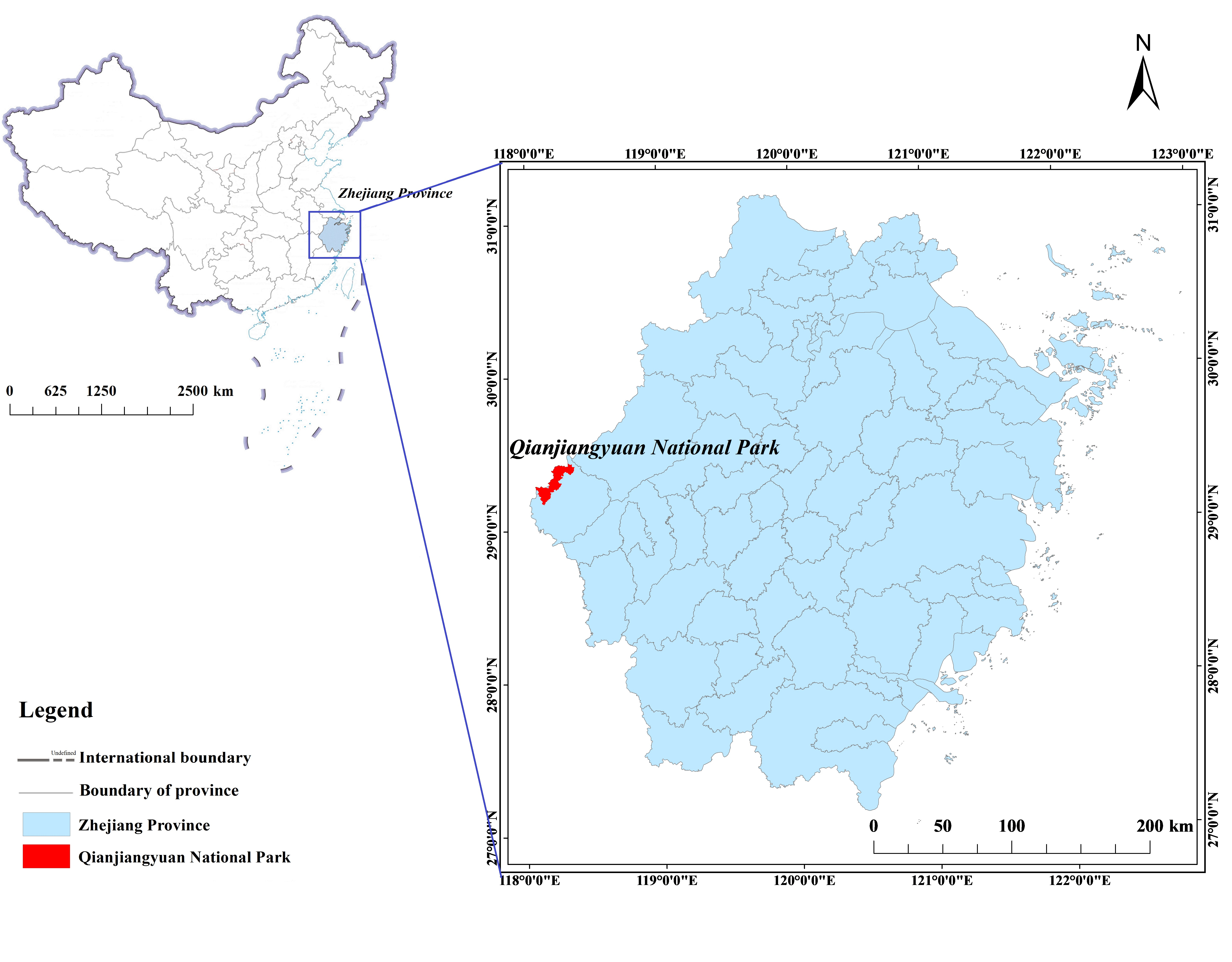
2.1. Study Area
2.2. Data Sources
2.2.1. Landscape Distribution Map of Qianjiangyuan National Park
2.2.2. Vegetation Type Distribution Map of Qianjiangyuan National Park
2.2.3. Habitat Identification and Dispersal Distance Threshold of Target Species
2.3. Data Processing
2.3.1. Landscape Fragmentation Analysis of Qianjiangyuan National Park
2.3.2. Key Habitat and Connectivity Analysis of Qianjiangyuan National Park
2.3.3. Potential Habitat Corridor Analysis of Qianjiangyuan National Park
3. Results
3.1. Analysis of Landscape Fragmentation
3.2. Morphological Spatial Pattern Analysis
3.3. The Delta of the Probability of Connectivity Analysis
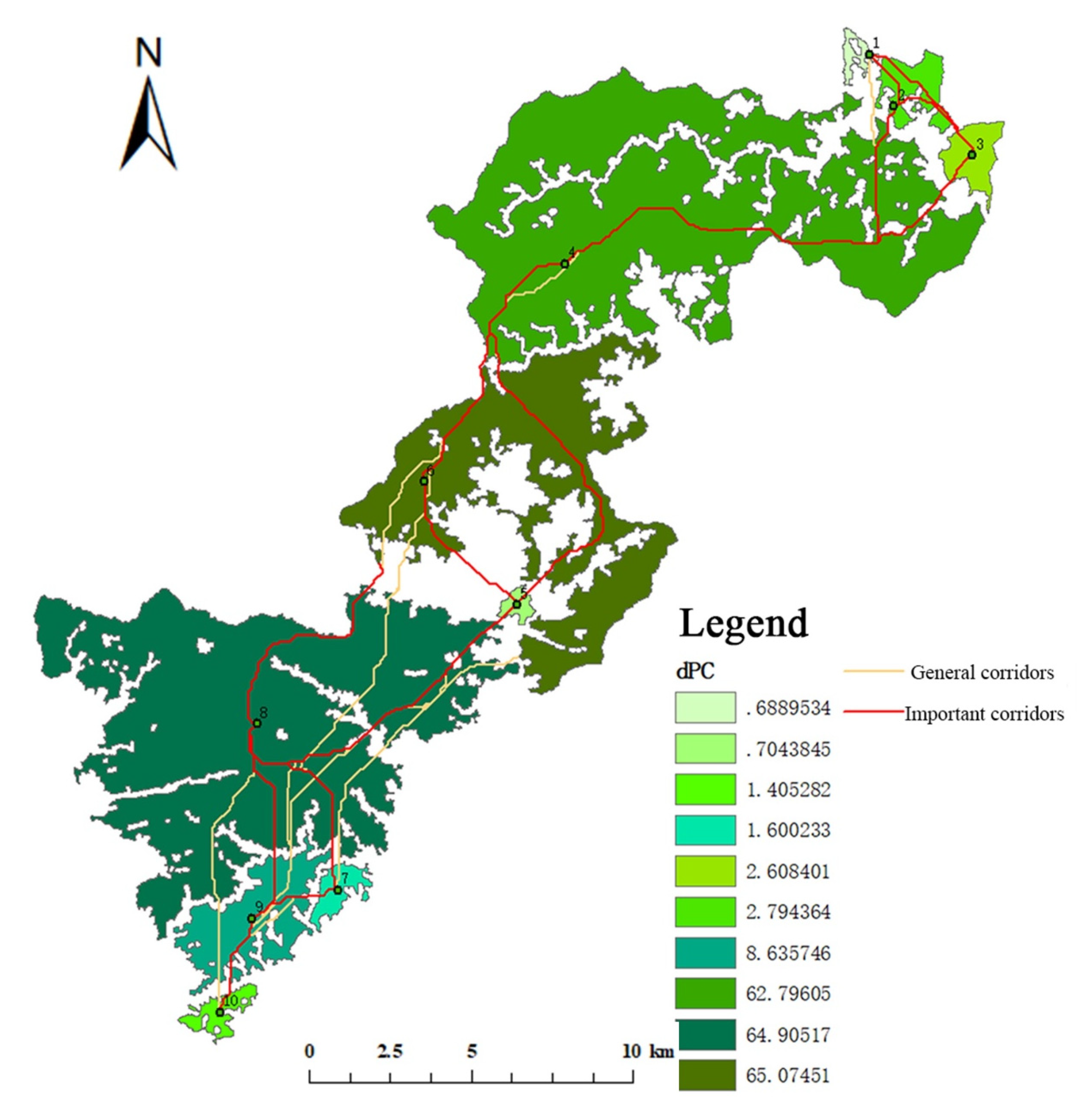
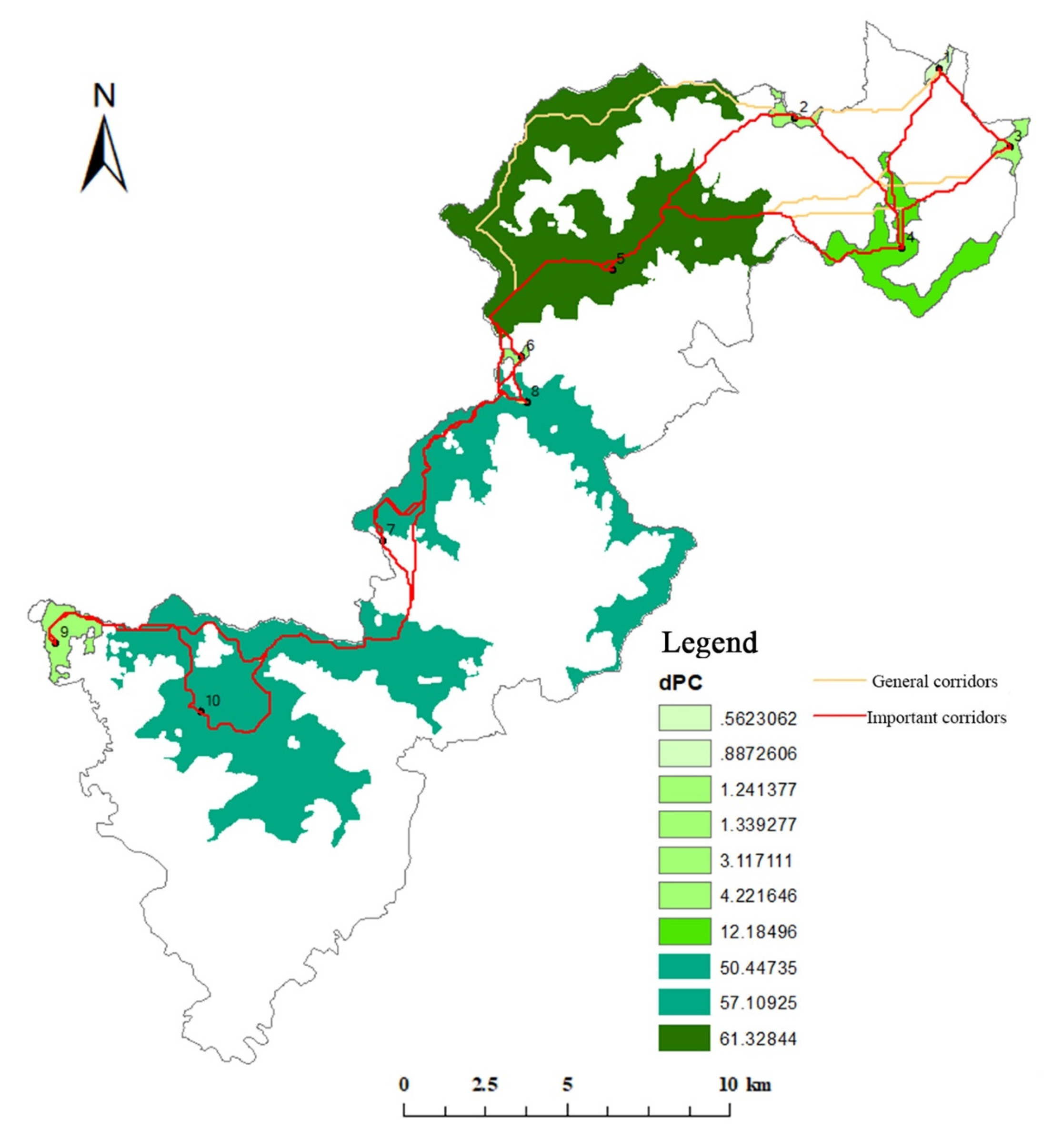
3.4. Analysis of Potential Habitat Corridors
3.5. Key Habitat and Important Corridor Network Analysis
4. Discussion
5. Conclusions
- (1)
- Roads, settlements, and cultivated land have a significant impact on the landscape connectivity of Qianjiangyuan National Park, with roads being one of the main reasons for the fragmentation of the overall landscape. We recommend that several potential corridors in the center of the park that connect key habitats on both sides of the road be protected to help link habitat patches, mitigate the impact of the road, and appropriate vegetation restoration and reforestation of tea plantations and drylands in the study area will increase the landscape connectivity of Qianjiangyuan National Park.
- (2)
- The area of each patch of key habitat is not proportional to its contribution to the landscape connectivity of Qianjiangyuan National Park, but the size of key habitats is important for maintaining landscape connectivity. At the landscape scale, large habitat patches of high importance should be prioritized for protection to promote habitat connectivity and species conservation in the study area. At the same time, groups of small patches with a high potential for species migration should also be protected as a whole to avoid further fragmentation or even area loss.
- (3)
- The locations and boundaries of strict protected areas and recreational areas of Qianjiangyuan National Park are relatively reasonable, and the scope of ecological conservation areas and traditional use areas could be adjusted to better match the distribution of key habitats. Special attention must be focused on protecting and managing ecological conservation areas because of the pressure of human disturbance around the area. However, at the same time, there are several important corridors in the area, and the connectivity between strictly protected areas depends on successful protection of ecological conservation areas.
Author Contributions
Funding
Institutional Review Board Statement
Informed Consent Statement
Data Availability Statement
Acknowledgments
Conflicts of Interest
References
- Ancillotto, L.; Bosso, L.; Conti, P.; Russo, D. Resilient responses by bats to a severe wildfire: Conservation implications. Anim. Conserv. 2020. [Google Scholar] [CrossRef]
- Zhang, G.; Zheng, D.; Wu, H.; Wang, J.; Li, S. Assessing the role of high-speed rail in shaping the spatial patterns of urban and rural development: A case of the Middle Reaches of the Yangtze River, China. Sci. Total Environ. 2020, 704, 135399. [Google Scholar] [CrossRef] [PubMed]
- Jordán, F. Adding function to structure—comments on Palmarola landscape connectivity. Community Ecol. 2001, 2, 133–135. [Google Scholar] [CrossRef]
- Magness, D.; Sesser, A.; Hammond, T. Using topographic geodiversity to connect conservation lands in the Central Yukon, Alaska. Landsc. Ecol. 2018, 33, 547–556. [Google Scholar] [CrossRef]
- Taylor, P.; Fahrig, L.; Henein, K.; Merriam, G. Connectivity Is a Vital Element of Landscape Structure. Oikos 1993, 68, 571–573. [Google Scholar] [CrossRef]
- Adriaensen, F.; Chardon, J.; De Blust, G.; Swinnen, E.; Villalba, S.; Gulinck, H.; Matthysen, E. The application of ‘least-cost’ modelling as a functional landscape model. Landsc. Urban Plan. 2003, 64, 233–247. [Google Scholar] [CrossRef]
- Wu, J. Landscape Ecology: Pattern, Process, Scale and Hierarchy, 2nd ed.; Higher Education Press: Beijing, China, 2007; ISBN 7-04-020879-2. [Google Scholar]
- He, J.; Huang, J.; Liu, D.; Wang, H.; Li, C. Updating the habitat conservation institution by prioritizing important connectivity and resilience providers outside. Ecol. Indic. 2018, 88, 219–231. [Google Scholar] [CrossRef]
- Cook, E.A. Landscape structure indices for assessing urban ecological networks. Landsc. Urban Plan. 2002, 58, 269–280. [Google Scholar] [CrossRef]
- Minor, E.S.; Lookingbill, T.R. A multiscale network analysis of protected-area connectivity for mammals in the United States. Conserv. Biol. 2010, 24, 1549–1558. [Google Scholar] [CrossRef]
- Machado, R.; Godinho, S.; Guiomar, N.; Gil, A.; Pirnat, J. Using graph theory to analyse and assess changes in Mediterranean woodland connectivity. Landsc. Ecol. 2020, 35, 1291–1308. [Google Scholar] [CrossRef]
- O’Leary, B.C.; Roberts, C.M. Ecological connectivity across ocean depths: Implications for protected area design. Glob. Ecol. Conserv. 2018, 15, e00431. [Google Scholar] [CrossRef]
- Job, N.; Roux, D.J.; Bezuidenhout, H.; Cole, N.S. A Multi-Scale, Participatory Approach to Developing a Protected Area Wetland Inventory in South Africa. Front. Environ. Sci. 2020, 8, 49. [Google Scholar] [CrossRef]
- Roberts, K.; Cook, C.; Beher, J.; Treml, E. Assessing the current state of ecological connectivity in a large marine protected area system. Conserv. Biol. 2020, 35, 699–710. [Google Scholar] [CrossRef]
- Cruz-Vazquez, C.; Rioja-Nieto, R.; Enriquez, C. Spatial and temporal effects of management on the reef seascape of a marine protected area in the Mexican Caribbean. Ocean Coast. Manag. 2019, 169, 50–57. [Google Scholar] [CrossRef]
- Amaral, Y.; Santos, E.; Ribeiro, M.; Barreto, L. Landscape structural analysis of the Lençóis Maranhenses National Park: Implications for conservation. J. Nat. Conserv. 2019, 51, 125725. [Google Scholar] [CrossRef]
- Lima, F.G.; Diniz, M.F.; Mendes, P. Ranking habitat importance for small wildcats in the Brazilian savanna: Landscape connectivity as a conservation tool. Biologia 2021, 76, 1–11. [Google Scholar] [CrossRef]
- Freeman, B.; Roehrdanz, P.R.; Peterson, A.T. Modeling endangered mammal species distributions and forest connectivity across the humid Upper Guinea lowland rainforest of West Africa. Biodivers. Conserv. 2018, 28, 671–685. [Google Scholar] [CrossRef]
- Bargelt, L.; Fortin, M.J.; Murray, D.L. Assessing connectivity and the contribution of private lands to protected area networks in the United States. PLoS ONE 2020, 15, e0228946. [Google Scholar] [CrossRef]
- Stewart, F.; Darlington, S.; Volpe, J.P.; Mcadie, M.; Fisher, J.T. Corridors best facilitate functional connectivity across a protected area network. Sci. Rep. 2019, 9, 10852. [Google Scholar] [CrossRef]
- Saura, S.; Bertzky, B.; Bastin, L.; Battistella, L.; Dubois, G. Global trends in protected area connectivity from 2010 to 2018. Biol. Conserv. 2019, 238, 1–8. [Google Scholar] [CrossRef]
- Huang, C.; Li, X.; Khanal, L.; Jiang, X. Habitat suitability and connectivity inform a co-management policy of protected area network for Asian elephants in China. PeerJ 2019, 7, e6791. [Google Scholar] [CrossRef] [PubMed]
- Wu, R.; Hua, C.; Yu, G.; Ma, J.; Yang, F.; Wang, J.; Jin, T.; Long, Y.; Guo, Y.; Zhao, H. Assessing protected area overlaps and performance to attain China’s new national park system. Biol. Conserv. 2020, 241, 108382. [Google Scholar] [CrossRef]
- McRae, B.H.; Shah, V.B. Circuitscape User Guide. The University of California, Santa Barbara. 2011. Available online: https://www.researchgate.net/publication/265494222 (accessed on 21 May 2021).
- McRae, B. Isolation by resistance. Evol. Int. J. Org. Evol. 2006, 60, 1551–1561. [Google Scholar] [CrossRef]
- Theobald, D.M. A general model to quantify ecological integrity for landscape assessments and US application. Landsc. Ecol. 2013, 28, 1859–1874. [Google Scholar] [CrossRef]
- Compton, B.; McGarigal, K.; Cushman, S.; Gamble, L. A Resistant-Kernel Model of Connectivity for Amphibians that Breed in Vernal Pools. Conserv. Biol. J. Soc. Conserv. Biol. 2007, 21, 788–799. [Google Scholar] [CrossRef] [PubMed]
- White, J.W.; Scholz, A.J.; Rassweiler, A.; Steinback, C.; Botsford, L.W.; Kruse, S.; Costello, C.; Mitarai, S.; Siegel, D.A.; Drake, P.T. A comparison of approaches used for economic analysis in marine protected area network planning in California. Ocean Coast. Manag. 2013, 74, 77–89. [Google Scholar] [CrossRef]
- Allen, C.H.; Parrott, L.; Kyle, C. An individual-based modelling approach to estimate landscape connectivity for bighorn sheep (Ovis canadensis). PeerJ 2016, 4, e2001. [Google Scholar] [CrossRef]
- Guo, S.; Kaoru, S.; Yin, W.; Chang, S. Landscape Connectivity as a Tool in Green Space Evaluation and Optimization of the Haidan District, Beijing. Sustainability 2018, 10, 1979. [Google Scholar] [CrossRef]
- Ding, P.; Zhuge, Y. Elliot’s Pheasant. Chin. J. Zool 1989, 24, 39–42. [Google Scholar] [CrossRef]
- Li, B. The Elliot’s pheasant in Southern Anhui. Chin. Wildl. 1985, 5, 18–20. [Google Scholar] [CrossRef]
- Shi, J. The seasonal changes of habitats of Elliot’s Pheasant. Zool. Res. 1997, 18, 275–283. [Google Scholar]
- Yanbo, P.; Ping, D. Factors Affecting Movement of Spring Dispersal of Elliot’s Pheasants. Zool. Res. 2005, 26, 373–378. [Google Scholar]
- Zhang, G. The Natural Dispersion and Habitat Selection of Syrmaticus Ellioti; Guangxi Normal University: Guilin, China, 2015. [Google Scholar]
- Zheng, X.; Bao, Y.; Ge, B.; Zheng, R. Seasonal changes in habitat use of black muntjac (Muntiacus crinifr ons) in Zhejiang. Acta Theriol. Sin. 2006, 26, 201–205. [Google Scholar] [CrossRef]
- Wang, Q. Anhui Chronicles of the Animals; Anhui Science & Technology Publishing House: Hefei, China, 1990; ISBN 7-5337-0410-5. [Google Scholar]
- Sheng, H. Chinese Deer Species; East China Normal University Press: Shanghai, China, 1992; ISBN 7-5617-0795-9/Q.008. [Google Scholar]
- Bennett, A.F.; Saunders, D. Habitat Fragmentation and Landscape Change; Oxford University Press: Oxford, UK, 2010; ISBN 9780191720666. [Google Scholar]
- Soille, P.; Vogt, P. Morphological segmentation of binary patterns. Pattern Recognit. Lett. 2009, 30, 456–459. [Google Scholar] [CrossRef]
- Saura, S.; Pascual-Hortal, L. A new habitat availability index to integrate connectivity in landscape conservation planning: Comparison with existing indices and application to a case study. Landsc. Urban Plan. 2007, 83, 91–103. [Google Scholar] [CrossRef]
- Guo, G.; Wu, Z.; Xiao, R.; Chen, Y.; Liu, X.; Zhang, X. Impacts of urban biophysical composition on land surface temperature in urban heat island clusters. Landsc. Urban Plan. 2015, 135, 1–10. [Google Scholar] [CrossRef]
- Grimm, N.B.; Faeth, S.H.; Golubiewski, N.E.; Redman, C.L.; Wu, J.; Bai, X.; Briggs, J.M. Global Change and the Ecology of Cities. Science 2008, 319, 756–760. [Google Scholar] [CrossRef]
- Zhang, J.; Liu, F.; Cui, G. The Efficacy of Landscape-Level Conservation in Changbai Mountain Biosphere Reserve, China. PLoS ONE 2014, 9, e95081. [Google Scholar] [CrossRef]
- Sklar, F.H.; Costanza, R. The development of dynamic spatial models for landscape ecology: A review and prognosis. Ecol. Stud. Anal. Synth. 1991, 82, 239–288. [Google Scholar] [CrossRef]
- Smeraldo, S.; Bosso, L.; Fraissinet, M.; Bordignon, L.; Brunelli, M.; Ancillotto, L.; Russo, D. Modelling risks posed by wind turbines and power lines to soaring birds: The black stork (Ciconia nigra) in Italy as a case study. Biodivers. Conserv. 2020, 29, 1959–1976. [Google Scholar] [CrossRef]
- Lhoest, S.; Fonteyn, D.; Danou, K.; Delbeke, L.; Fayolle, A. Conservation value of tropical forests: Distance to human settlements matters more than management in Central Africa. Biol. Conserv. 2020, 241, 108351. [Google Scholar] [CrossRef]
- Del Carmen Sabatini, M.; Verdiell, A.; Rodríguez Iglesias, R.M.; Vidal, M. A quantitative method for zoning of protected areas and its spatial ecological implications. J. Environ. Manage. 2007, 83, 198–206. [Google Scholar] [CrossRef]
- Fu, M. Identification of functional zones and methods of target management in Sanjiangyuan National Park. Biodivers. Sci. 2017, 25, 52–63. [Google Scholar] [CrossRef]
- Fu, M.; Tian, J.; Ren, Y.; Li, J.; Liu, W.; Zhu, Y. Functional zoning and space management of Three-River-Source National Park. J. Geogr. Sci. 2019, 29, 2069–2084. [Google Scholar] [CrossRef]
- Habtemariam, B.T.; Fang, Q. Zoning for a multiple-use marine protected area using spatial multi-criteria analysis: The case of the Sheik Seid Marine National Park in Eritrea. Mar. Policy 2016, 63, 135–143. [Google Scholar] [CrossRef]
- Ruiz-Labourdette, D.; Schmitz, M.F.; Montes, C.; Pineda, F.D. Zoning a Protected Area: Proposal Based on a Multi-thematic Approach and Final Decision. Env. Model Assess 2010, 15, 531–547. [Google Scholar] [CrossRef]
- Verdiell, A.; Sabatini, M.C.; Maciel, M.C.; Iglesias, R. A mathematical model for zoning of protected natural areas. Int. Trans. Oper. Res. 2005, 12, 203–213. [Google Scholar] [CrossRef]
- Hilty, J.; Worboys, G.L.; Keeley, A.; Woodley, S.; Lausche, B.J.; Locke, H.; Carr, M.; Pulsford, I.; Pittock, J.; White, J.W.; et al. Guidelines for Conserving Connectivity Through Ecological Networks and Corridors; IUCN: Gland, Switzerland, 2020; ISBN 9782831720524. [Google Scholar]
- Noss, R.F.; Harris, L.D. Nodes, networks, and MUMs: Preserving diversity at all scales. Environ. Manag. 1986, 10, 299–309. [Google Scholar] [CrossRef]


| Landscape Index | Abbreviation | Formula | Description |
|---|---|---|---|
| Percentage of protected landscape patch area | P | Range: 0 ≤ P ≤ 1; is the area of the i-th protected landscape patch; A is the total area of the national park | |
| Area weighted mean plaque fractal dimension [6,23] | AWMPFD | Range: 1 ≤ AWMPFD ≤ 2; is the perimeter of the j-th patch of type i, is the area of the j-th patch of type i | |
| Fragmentation index | F | Range: 0 ≤ F ≤ 1; is the area of the i-th protected landscape patch | |
| Relative aggregation [6,24] | C′ | Range: 0 ≤ C′ ≤ 1; is the perimeter of the j-th patch of the i-th type, n is the total number of patch types in the landscape |
| Serial Number | Landscape Category | Area (km2) | Proportion (%) |
|---|---|---|---|
| 1 | Natural arboreal forest | 205.6821 | 78.3672 |
| 2 | Tea plantation | 19.43847 | 7.4063 |
| 3 | Dry land | 11.51652 | 4.3879 |
| 4 | Shrubland | 10.41074 | 3.9666 |
| 5 | Bamboo forest | 7.481252 | 2.8504 |
| 6 | River | 2.380823 | 0.9071 |
| 7 | Reservoir | 1.828854 | 0.6968 |
| 8 | Highway | 1.007906 | 0.3840 |
| 9 | Rural residential land | 0.973664 | 0.3710 |
| 10 | Trail | 0.586553 | 0.2235 |
| 11 | Natural grassland | 0.393852 | 0.1501 |
| 12 | Bare land | 0.264007 | 0.1006 |
| 13 | Other forest land | 0.107711 | 0.0410 |
| 14 | Urban residential land | 0.100458 | 0.0383 |
| 15 | Nursery land | 0.099273 | 0.0378 |
| 16 | Road land | 0.057231 | 0.0218 |
| 17 | Other construction land | 0.037765 | 0.0144 |
| 18 | Detached house | 0.035179 | 0.0134 |
| 19 | House under construction | 0.018213 | 0.0069 |
| 20 | Pond | 0.017469 | 0.0067 |
| 21 | Lake | 0.006537 | 0.0025 |
| 22 | Land for hydraulic Construction | 0.005876 | 0.0022 |
| 23 | Ditch | 0.004842 | 0.0018 |
| 24 | Bridge | 0.004084 | 0.0016 |
| 25 | Aggregate | 252.3800 | 100 |
| Serial Number | Landscape Index | Result |
|---|---|---|
| 1 | Percentage of protected landscape area (P) | 0.87 |
| 2 | Area-weighted average plaque fractal dimension (AWMPFD) | 1.38 |
| 3 | Fragmentation index (F) | 0.51 |
| 4 | Relative degree of aggregation (C′) | 0.69 |
| Species | Land Cover Type/Vegetation | Altitude | Slope | Distance from Road | Distance from Residence |
|---|---|---|---|---|---|
| Elliot’s Pheasant | Broad-leaved forests, coniferous forest, mixed forests, bamboo forests, shrub forests, farmland | 200–1900 m | ≤50° | >700 m | >700 m |
| Black Muntjac | Broad-leaved forests, mixed forests, coniferous forests, shrub forests | ≥600 m | ≤45° | ≥50 m | ≥200 m |
| Patch Number | Elliot’s Pheasant | Black Muntjac | ||
|---|---|---|---|---|
| dPC | Area (km2) | dPC | Area (km2) | |
| 1 | 65.07451 | 32.32 | 61.32844 | 30.31 |
| 2 | 64.90517 | 66.47 | 57.10925 | 31.92 |
| 3 | 62.79605 | 67.47 | 50.44735 | 17.66 |
| 4 | 8.635746 | 7.96 | 12.18496 | 5.57 |
| 5 | 2.794364 | 2.76 | 4.221646 | 1.99 |
| 6 | 2.608401 | 2.54 | 3.117111 | 0.22 |
| 7 | 1.600233 | 1.54 | 1.339277 | 0.64 |
| 8 | 1.405282 | 1.39 | 1.241377 | 0.72 |
| 9 | 0.704385 | 0.66 | 0.887261 | 0.01 |
| 10 | 0.688953 | 0.67 | 0.562306 | 0.35 |
| Rating | Vegetation | Altitude | Gradient | Distance from Road | Distance from Residence | Resistance | Cost Value |
|---|---|---|---|---|---|---|---|
| Most suitable | Broadleaf forests, mixed forests | 300–800 m | 0–30° | >1800 m | >2200 m | 0 | 1 |
| Suboptimal | Coniferous forests, bamboo forests | 200–300 m; 800–1000 m | 30–40° | 1000–1800 m | 1500–2200 m | 0.38 | 38 |
| Generally appropriate | Shrublands, farm lands | 1000–1900 m | 40–50° | 700–1000 m | 700–1500 m | 0.62 | 62 |
| Unsuitable | others | <200 m; >1900 m | >50° | <700 m | <700 m | 1 | 100 |
| Rating | Vegetation | Altitudes | Gradient | Distance from Road | Distance from Residence | Resistance | Cost Value |
|---|---|---|---|---|---|---|---|
| Most suitable | Broadleaf forests, mixed forests | 800–1000 m | 0–30° | >600 | >1000 | 0 | 1 |
| Suboptimal | Coniferous forests, shrublands | 600–800 m; 1000 | 30–45° | 200–600 | 500–1000 m | 0.38 | 38 |
| Generally appropriate | — | — | — | 50–200 | 200–500 | 0.62 | 62 |
| Unsuitable | Bamboo forests, meadows, other | <600 m; | >45° | <50 | <200 m | 1 | 100 |
| Key Habitat Number | 1 | 2 | 3 | 4 | 5 | 6 | 7 | 8 | 9 | 10 |
|---|---|---|---|---|---|---|---|---|---|---|
| 1 | 0.93 | 0.19 | 0.06 | 0.01 | 0.04 | 0.0050 | 0.01 | 0.0067 | 0.0034 | |
| 2 | 0.48 | 0.12 | 0.02 | 0.07 | 0.0080 | 0.02 | 0.01 | 0.0053 | ||
| 3 | 0.10 | 0.02 | 0.06 | 0.0070 | 0.02 | 0.0092 | 0.0047 | |||
| 4 | 0.15 | 1.48 | 0.03 | 0.09 | 0.03 | 0.02 | ||||
| 5 | 0.29 | 0.03 | 0.10 | 0.04 | 0.01 | |||||
| 6 | 0.08 | 0.30 | 0.09 | 0.04 | ||||||
| 7 | 0.49 | 0.62 | 0.09 | |||||||
| 8 | 0.54 | 0.11 | ||||||||
| 9 | 0.40 | |||||||||
| 10 |
| Key Habitat Number | 1 | 2 | 3 | 4 | 5 | 6 | 7 | 8 | 9 | 10 |
|---|---|---|---|---|---|---|---|---|---|---|
| 1 | 0.08 | 0.29 | 0.26 | 0.09 | 0.04 | 0.02 | 0.06 | 0.03 | 0.03 | |
| 2 | 0.06 | 0.18 | 0.23 | 0.09 | 0.04 | 0.12 | 0.04 | 0.03 | ||
| 3 | 0.39 | 0.10 | 0.04 | 0.03 | 0.07 | 0.04 | 0.03 | |||
| 4 | 0.39 | 0.15 | 0.07 | 0.21 | 0.08 | 0.06 | ||||
| 5 | 4.23 | 0.64 | 2.94 | 0.22 | 0.18 | |||||
| 6 | 0.91 | 9.34 | 0.17 | 0.14 | ||||||
| 7 | 2.64 | 0.19 | 0.16 | |||||||
| 8 | 0.33 | 0.28 | ||||||||
| 9 | 10.00 | |||||||||
| 10 |
Publisher’s Note: MDPI stays neutral with regard to jurisdictional claims in published maps and institutional affiliations. |
© 2021 by the authors. Licensee MDPI, Basel, Switzerland. This article is an open access article distributed under the terms and conditions of the Creative Commons Attribution (CC BY) license (https://creativecommons.org/licenses/by/4.0/).
Share and Cite
Peng, Y.; Meng, M.; Huang, Z.; Wang, R.; Cui, G. Landscape Connectivity Analysis and Optimization of Qianjiangyuan National Park, Zhejiang Province, China. Sustainability 2021, 13, 5944. https://doi.org/10.3390/su13115944
Peng Y, Meng M, Huang Z, Wang R, Cui G. Landscape Connectivity Analysis and Optimization of Qianjiangyuan National Park, Zhejiang Province, China. Sustainability. 2021; 13(11):5944. https://doi.org/10.3390/su13115944
Chicago/Turabian StylePeng, Yangjing, Minghao Meng, Zhihao Huang, Ruifeng Wang, and Guofa Cui. 2021. "Landscape Connectivity Analysis and Optimization of Qianjiangyuan National Park, Zhejiang Province, China" Sustainability 13, no. 11: 5944. https://doi.org/10.3390/su13115944
APA StylePeng, Y., Meng, M., Huang, Z., Wang, R., & Cui, G. (2021). Landscape Connectivity Analysis and Optimization of Qianjiangyuan National Park, Zhejiang Province, China. Sustainability, 13(11), 5944. https://doi.org/10.3390/su13115944