Prediction of Depth of Seawater Using Fuzzy C-Means Clustering Algorithm of Crowdsourced SONAR Data

Abstract

Implementing AI in all fields is a solution to the complications that can be troublesome to solve for human beings and will be the key point of the advancement of those spheres. In the marine world, specialists also encounter some problems that can be revealed through addressing AI and machine learning algorithms. One of these challenges is determining the depth of the seabed with high precision. The depth of the seabed is utterly significant in the procedure of ships at sea occupying a safe route. Thus, it is considerably crucial that the ships do not sit in shallow water. In this article, we have addressed the fuzzy c-means (FCM) clustering algorithm, which is one of the vigorous unsupervised learning methods under machine learning to solve the mentioned problems. In the case study, crowdsourced data have been trained, which are gathered from vessels that have installed sound navigation and ranging (SONAR) sensors. The data for the training were collected from ships sailing in the south part of South Korea. In the training section, we segregated the training zone into the diminutive size areas (blocks). The data assembled in blocks had been trained in FCM. As a result, we have received data separated into clusters that can be supportive to differentiate data. The results of the effort show that FCM can be implemented and obtain accurate results on crowdsourced bathymetry.

1. Introduction

Smart technologies and smart approaches to unraveling problems are gradually reaching all the works that individuals do. Therefore, it can be surely emphasized that the perspective of our lifestyle and the objects surrounding us are the result of the implementation of artificial intelligence, machine learning, Big Data, cloud computing, remote sensing, and the Internet of Things [1]. Thus, we are trying to furnish every branch of our world with novel technologies, and as a result, in time new concepts and solutions for smart things [2], smart environments, smart vehicles, and smart cities are being introduced and broadened. This sort of wave of technologies is also being presented into the marine world. Concepts of smart ships [3,4,5] and smart ports [6,7] as well as presented applications [8,9,10] for them can be classical proof of the pointed-out expressions.

The evolution of the applications and systems for the vessels and ports plays an essential role in the forthcoming life of a marine economy and safety. Especially, for the safety of the vessels, crews, and passengers, smart solutions to the marine represent an enormous impact. One of the accidental and hazardous circumstances at sea for vessels is the sinking of the ship in a shallow area at sea. To avoid this situation, the ships move in directions that are secure for them, i.e., the depth of the seabed is known in advance. This exposes that determining the depth of the seabed is highly consequential for the riskless movement of ships. Additionally, for comprehending ocean circulation, environmental changes, underwater geo-hazards, tsunamis, resources, and many other processes affected by the environment, commerce and safety are satisfactory to grasp and understand seafloor and depth of water [11]. That is why numerous countries bordering water regularly check the sea depths at close distances to ensure the safety of ships moving at sea. The tasks like measuring the depth of the sea are predominantly carried out by specific government organizations. The proceeding of measuring the depth of the seabed provides echo-sounding, which is one of the most reliable methods for calculating the depth of the seafloor. Nevertheless, checking the underwater depth over a large area is a toilsome and time-consuming task. Given that water flows in the lower part of the sea change the position of sand dunes on the seabed, the sea depth will need to be measured regularly. Therefore, it is desirable to perform this task not only through a small number of sources (such as one or two organizations) but also through many sources (crowdsourcing). International organizations such as the International Hydrographic Organization (IHO) and International Marine Organization (IMO) also rate the crowdsourcing method as positive in determining sea depth. However, data gathered from many sources generate a very large amount of data (Big Data), and at the same time, there will be numerous noisy (inaccurate) data within the Big Data. As highlighted above, artificial intelligence and machine learning algorithms can be used to efficiently sort out Big Data from erroneous data and obtain the exact information we require. One of the most regularly utilized approaches for classifying unlabeled noisy data is the clustering method. Data clustering algorithms come under unsupervised learning. There are several sorts of clustering methods; however, in this work, we employed fuzzy-logic-based fuzzy c-means clustering. It is similar to k-means clustering, but the only difference is that, unlike k-means, c-means is not a hard clustering, but it is a soft clustering [12]. The primary dissimilarity between hard and soft clustering is that in hard clustering, a single data point in the entire dataset belongs to only one cluster, while in soft clustering, a single data point can belong to multiple clusters with a membership value. We can affirm that the fuzzy-logic-based soft clustering is an improved version of k-means, which represents the amenity of providing more accurate results, especially in an overlapped data. In this paper, we applied FCM clustering to sort noisy crowdsourced sea depth data. A case-study experiment was done with data gathered from the ships that are sailing nearby the south part of South Korea. According to the results, the FCM algorithm can be implemented to measure the depth of the sea and pass over reliable results.

The research work contribution is as follows:

• The fuzzy-logic-based FCM algorithm was implemented in the field to predict depth data.
• The proposed method obtained more accurate depth data by clustering the data, which is experimentally proven.
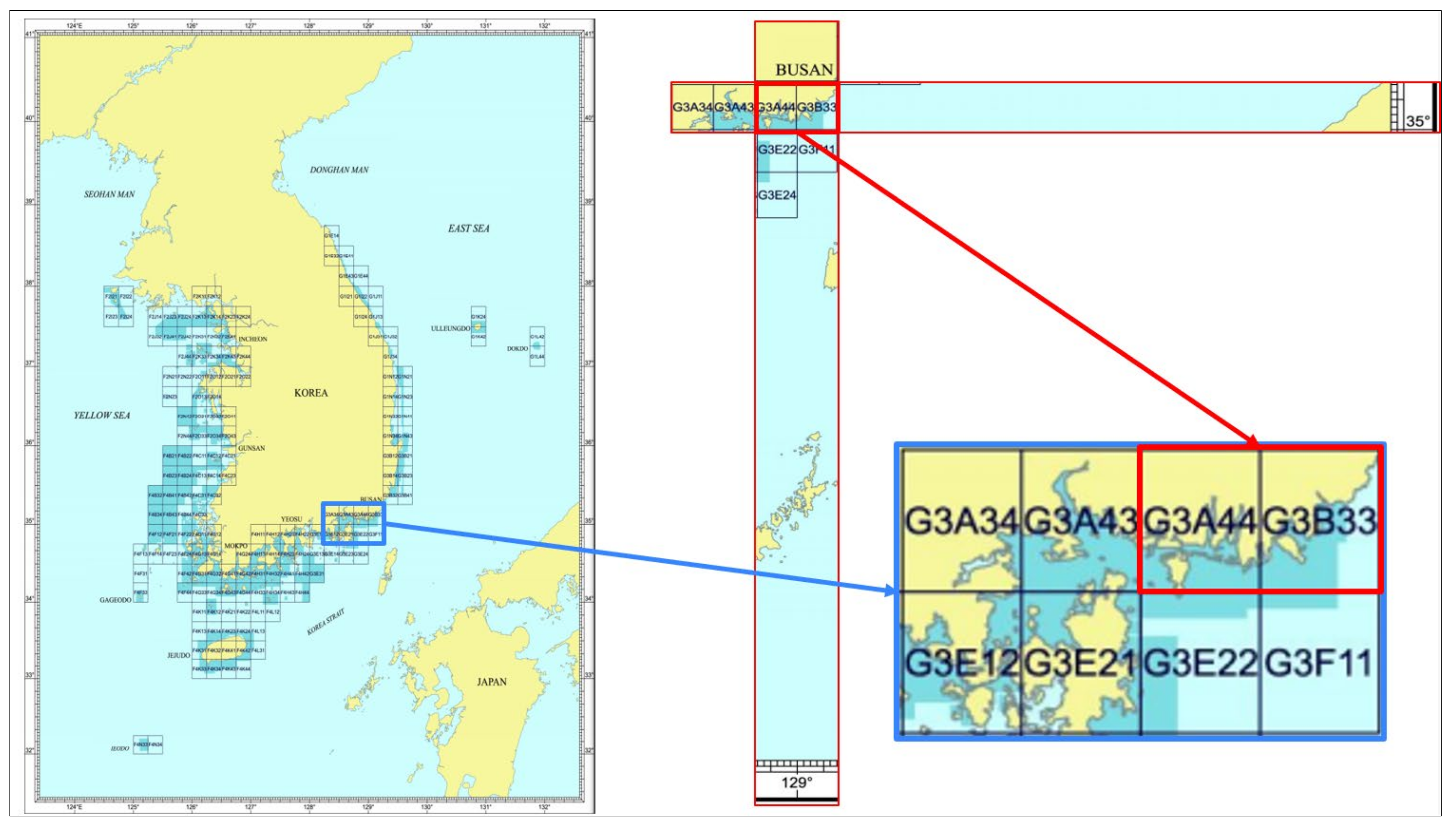
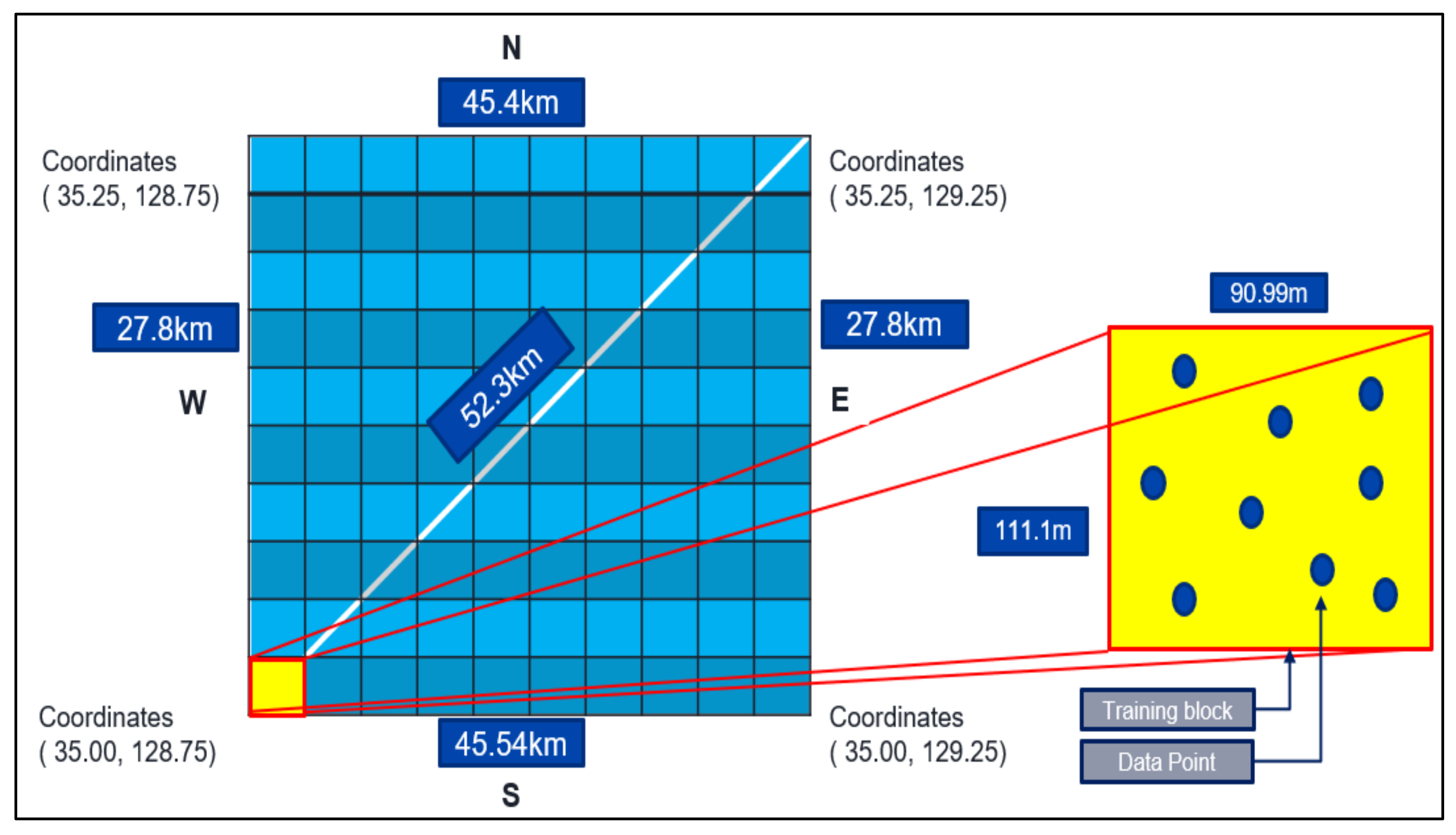
• To obtain accurate results, the proposed model divided the data into the parts (blocks) with sizes approximately 100 to 100 m by location of the data measurements according to domain knowledge.
• The accuracy of the proposed model was measured by calculating the mean absolute error of the mean value of each block of the real data and the FCM value of each block.

After going through the introduction of the work in Section 1, the rest of the paper includes the following sections: Section 2 presents the related works about measuring the depth of sea or ocean water and works about data clustering with fuzzy logic. Section 3 describes the materials and method of the current research work. Section 4 illustrates the results of the experiment. Finally, the conclusions of this research and future work are presented in Section 5.

2. Related Works

In the marine field, particularly in the field of waterway navigation and transportation, this research work is dedicated to the prediction of the depth of seawater. Big Data gathered in real time through automatic identification systems (AIS) by utilizing SONAR might provide a solution to predict error-free depths of the seabed. In order to offer accurate real-time information about the depth, the noisy Big Data must be separated from improper data. For this task, we addressed a fuzzy-logic-based clustering algorithm; however, this is not the only method to measure and forecast the depth of seawater. There are diverse sorts of research such as measuring sound (with a single beam (SBES) and multibeam echo sounders (MBES)), such as in our case, or light (including satellite-derived bathymetry (SDB), light detection and ranging (LiDAR), and satellite altimetry) on this entire topic [13]. Depth information obtained by analyzing satellite images shortly, SDB, is one of them, and in this type of research, several works have been already presented. For instance, in [14], a mapping approach for shallow water bathymetry was developed using random forest machine learning and multi-temporal satellite images to create a generalized depth estimation model. Caballero et al. [15] pointed out an assessment of the SDB depth limit caused by turbidity as determined with the reflectance of the red-edge bands at 709 nm (OLCI) and 704 nm (MSI) and a standard ocean color chlorophyll concentration. In [16], the authors demonstrated an overview of the current state of spaceborne-based remote sensing techniques used to approximate the topography and bathymetry of beaches and intertidal and nearshore areas. Moreover, Sue et al. [17] used multi-spectral satellite images to foretell water depth change along a waterway. Additionally, most of the studies [18,19,20,21,22,23,24,25] have been proposed with this remote sensing method for bathymetric measurement, which used multi-spectral or hyper-spectral sensors. Another method for bathymetry is LiDAR. A scanning LiDAR bathymetry has been promoted for airborne hydrographic surveying. The system has depth penetration capability of four optical diffuse attenuation lengths, with an accuracy of ±0.3 m. From an altitude of 500 m, the system generates a swath 270 m wide and a uniform sounding density on a 35 m grid spacing, with a placement accuracy of approximately 15 m [26]. Wilson et al. in [27] proposed that their algorithms and procedures were expanded for generating seafloor relative reflectance, together with a suite of shape-based waveform features from experimental advanced airborne research LiDAR-B. Irish and White [28] proposed and delineated the Scanning Hydrographic Operational Airborne LiDAR Survey system describing both LiDAR technology and the survey system. Wang et al. [29] made a comparison of six algorithms for single-wavelength bathymetric waveform processing, i.e., peak detection, the average square difference function, Gaussian decomposition, quadrilateral fitting, Richardson–Lucy deconvolution, and Wiener filter deconvolution. Authors in [30,31,32,33] utilized both satellite imagery and LiDAR, and authors in [34] addressed both high-resolution multispectral satellite and multibeam SONAR data to estimate bathymetry and introduce their research work. The above-illustrated works are dedicated to measuring and learning the depth of seawater with heterogeneous methods, but most of them are methodologies about how to measure and why to measure the depth. Notwithstanding, there are also works that announced their methods and algorithms to obtain more productive data. As a pattern of this, it can be highlighted that a gamma test is used to rank the relative significance of the model inputs and detect the best input combinations before the data-driven models are calibrated. Three data-driven models, i.e., the back-propagation artificial neural network, support vector machines, and the power function model are used to predict the variations of the groundwater depth as well as the performances of the three established models, which are further compared. Twelve indices, including natural, anthropic, biological, economic, and social factors that may influence the groundwater depth, are taken into consideration as the input of the data-driven models. The study is carried out in the plain of Shijiazhuang, the capital city of Hebei province in North China [35]. Yang, F in [36] recommended a deep neural network (DNN) based on a model, entitled DDTree, for using the real-time AIS data and the data from Global Mapper to prognosticate waterway depth for ships in an accurate and time-saving way. The model puts together a decision tree and DNN, which is trained and tested on the AIS and Global Mapper data from the Nantong and Fangcheng ports on the southeastern and southwestern coast of China. The actual waterway depth data were used together with the AIS data as the input to DDTree. In order to enhance the exactness of predicting the depth of water, Kang et al. [37] proposed a differential dynamic positioning algorithm based on GPS/Beidou that realizes middle precision based on low-cost equipment. Kisi and Shiri et al. [38] proposed their improved wavelet-neuro-fuzzy model by associating two methods, the discrete wavelet transform and the neuro-fuzzy model. As we noted, the prediction of the depth of seawater can be a component of some bigger systems targeted at avoiding ship collisions and marine traffic accidents. Vodas et al. [39] proposed his model that can predict a ship accident and has the ability to make a considered decision by using the AIS data. Li et al. [40] proposed his work on improving equipment for a collection of the AIS data. Finally, Yang et al. [41] highlighted a general review and summarized the main contributions of the AIS data for marine navigation safety.

3. Materials and Methods

3.1. Observation Technology of Depth of Seawater

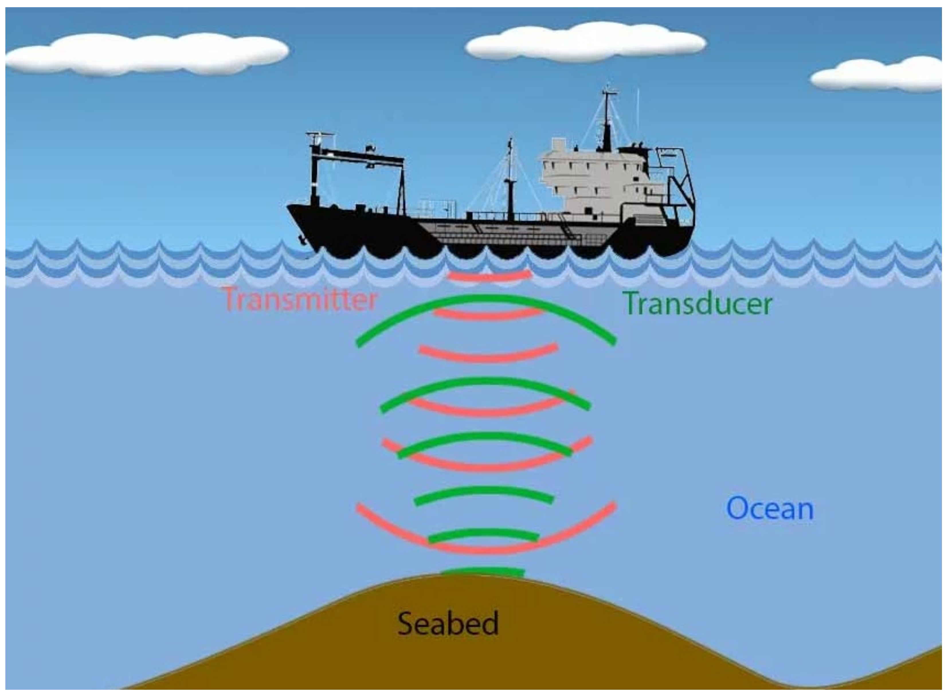
3.1.1. SONAR

In the marine field, learning and measuring the depth of the sea has been started since we have taken the safety of ships in the ocean more into consideration. Notwithstanding, before the invention of technologies like SONAR, humanity employed the technologies to measure the depth of seabed, which work manually. The earliest measuring method was “soundings”. A sounding line (a rope that has a weight fixed) is brought down over the side of the ship. As soon as the weight reaches the seafloor, the line starts to slow down and is determined at the water’s surface. Then, the weight is hauled back up, and the remoteness from the surface mark to the weight is calculated. The measured length is tantamount to the depth of the ocean at that place [42]. Initial primordial maps of the seafloor emerged from “soundings” [43]. Those primitive maps had very limited features as they illustrated only the overall image of the ocean floor, and only the bigger features could be pinpointed through looking for the patterns of the great number of such soundings. Many of those investigations were devoted to pointing out endangerment while shipping near the shore. The great number of soundings in deep water was analyzed by the expeditions that were done in the late 19th century. Figure 1 illustrates the first map of a seabed measured by sounding [44].

Sounding data were reliable; nonetheless, that method was complicated, affordable, and required plenty of time as well, particularly in the point of measuring very deep water.

The invention of SONAR switched the approach to mapping the seafloor. The SONAR is a sort of technology that has a transmitter that sends a sound pulse to the water and a receiver that detects the echo impulse that reaches and comes back from the depth of the ocean. The time difference from pulse to echo can be measured with analog means and directly gives depth. Receiving the echoes verifies the depth of the water, as in shallow water, the sound will revert very quickly, and in deeper water, it will require more time to obtain the echoes. By being acquainted with the sound speed in the water (approximately 1.5 km per second), the depth of the ocean can be calculated. This method of seafloor mapping is also known as single-beam echo-sounding [42,45]. This measuring method called multi-beam SONAR echo-sounding is an upgraded version of the single-beam. The multi-beam was cultivated to represent more accurate results of measuring; however, the working principles are closely identical to the single-beam, that is, sending sounds and receiving them, and after that calculating distance by utilizing time and speed of sound in the water. In Figure 2 below, we can see how the SONAR system works.

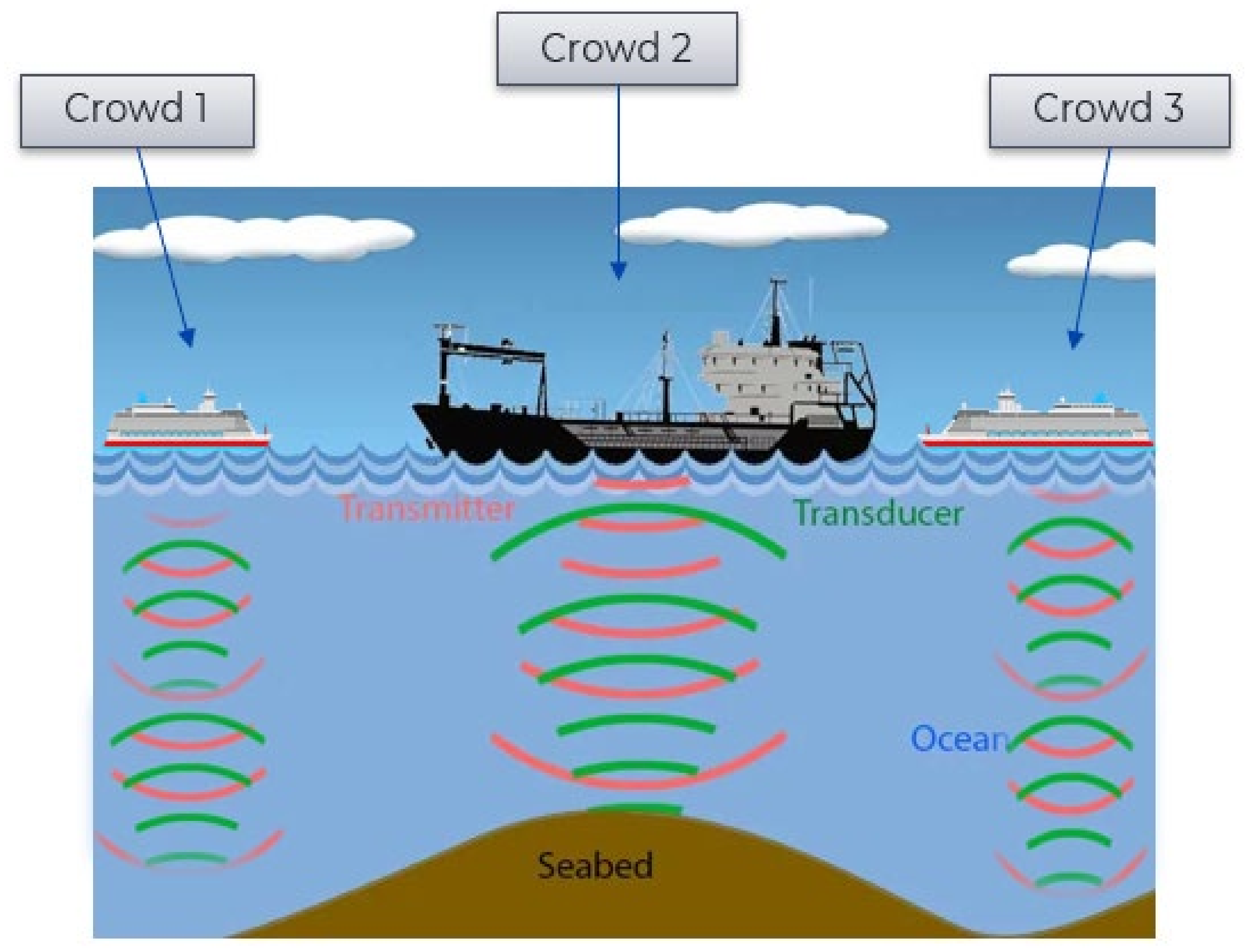
3.1.2. Crowdsourced Bathymetry

Through utilizing SONAR technology, it is aimed to obtain the amenity to obtain virtually 100% accurate depth of ocean data for a particular point by measuring that point a number of times with SONAR. Despite this, accomplishing by that huge amount of time is dissipated, as the surface of the sea is adequately immense, which equals approximately 362 million square kilometers, which are more than 70% of the surface of the Earth according to Eakins and Sharman in [46]. Therefore, the mapping of the seabed with only one or a few sources is difficult because they are so large, and here in this situation, we need more sources that can give us more data to use. Here comes crowdsourced bathymetry. The crowdsourcing bathymetry concept and guidance for it was developed by IHO. The bathymetry deals with the topography of the seabed as we mentioned before. In the data mining and Big Data world, when you do not have enough information or reliable data, there is a way to gather data with crowdsourcing. The authors of the work in [47] have published a high-quality survey about crowdsourcing. Crowdsourcing is obtaining data from each node that is connected and works under the same network. In bathymetry, the scenario crowd is the collection of vessels that have SONAR or a kind of technology that can measure and give reliable data about the depth of the seafloor. In this way, it is possible to collect a relatively large number of bathymetric data in a relatively short time, all at low cost. See Figure 3 below.

Crowdsourced bathymetry (CSB) is a comparatively up to date concept of accumulation bathymetric data, and it can be determined as the gathering as well as distributing of depth data (and metadata) measured and accumulated through distinctive survey vessels that are supplied with navigation devices in the procedure of prolonging their regular functions at sea [48].

In order to obtain a wider understanding of the bathymetry of the coastal waters and oceans, the IHO encouraged advanced methods to collect data and data maximizing initiatives. In 2014, the IHO, at its conference, announced that conventional survey vessels could not be counted upon to unravel data lacking matters and approved of encouraging and assisting mariners in an effort to “map the gaps” [13]. Crowdsourcing bathymetry is not a fully standardized bathymetric data collection process; however, the IHO set out the basic principles and technical requirements that related to the CSB.

Example of technical requirements for vessels for those who want to join crowdsourcing bathymetry voluntarily [48]:

• Vessels should be equipped with a global navigation satellite system (GNSS) for the calculation of the location and single-beam echo sounders (SBAS) for measurement of depth.
• The equipment (software and hardware) of the vessels must meet the recommendations of the IMO on performance standards so that vessels have the ability to gather bathymetric data (along with location and time) of standardized reliability.
• The collected data from GNSS and SBES on ships will be transferred to the National Marine Electronics Association (NMEA) and must be saved on board. Saved data will be transferred from vessels to the trusted node.
  For the purpose of achieving the required level of standardization, the IHO Data Center for Digital Bathymetry accepts bathymetric information in specific (default) formats. These formats are the CSV, XYZT, or GeoJson format. The XYZT format contains longitude, latitude, depth, and time. On depth measurement, the vertical distance between the line of the water surface and the thrust position of the SONAR transducer can play a significant role. Therefore, the IHO automatically recommends setup sensors according to the issue. The data collected in this way have a significant value in a whole range of activities related to improving seabed mapping.

3.2. Problem Analysis

One of the primary disadvantages of amassing data with crowdsourcing is that the system that is assembling data from all nodes may pick up and gather unverified data from some unidentified nodes. In the above scenario, nodes are vessels. The information that the chief database system accepts could be unexpectedly received from any member of the crowd due to technical or other complications, and the database system does not become aware of and cannot be able to verify which member of the crowd is gathering and sending the wrong data. As we indicated several times above, measuring sea or ocean depth with SONAR is transmitting echo sounds from the sender underwater to the seabed and getting back to the receiver. Within the procedure, if the wave does not encounter any obstacle underwater, it is possible to accurately gauge the seabed, since measuring the depth depends on how long the wave travels under the water. Figure 4a highlights precisely measuring sea depth.

What happens if a wave hits an obstacle between the surface of the sea and the bottom of the sea before it reaches the bottom of the sea? In this case, the measured point data is incorrectly retrieved and sent to the database. Such errors can be caused by a variety of trashes under the water, sea creatures, and even by fish. See Figure 4b. In addition to the above, there are other circumstances that could lead to improper data measurement. One of them is that these echo sounds are directed to the seabed at the wrong angle. These conditions can be caused by a strong sea wave at the sea surface or improper installation of SONAR sensors due to a technical error such as by the incorrect position of the sensor relative to the sea surface. See Figure 4c.

Given the aforementioned cases, it is natural that there is a huge quantity of inaccurate information among the crowdsourced data collected with a SONAR transducer. Therefore, it is obligatory to sort the collected data utilizing crowdsourcing and separate the accurate data from it. The next part discusses what sort of solutions can be implemented to disentangle these complications in such a situation.

3.3. Possible Solutions

As it is pointed out, the paramount task is to classify the sea depth data, which are gathered through crowdsourcing. In order to reveal the task, we need data from sensors. The sensors attached to the ships are able to provide not only information respecting the depth of the seabed, but also can illustrate water temperature, wind speed, ship speed, ship location within the transmission, etc. However, since we have to calculate the depth of the sea, it is enough to be acquainted with the geographical location of the ship and the depth of the sea at that point.

Table 1. Example of depth data of same location.

Latitude	Longitude	Depth(m)
35.136863	129.192551	10
35.136863	129.192551	11
35.136863	129.192551	20
35.136863	129.192551	23
35.136863	129.192551	21
35.136863	129.192551	20

shows patterns of depth data of the same location by these two data types.

As illustrated in the table above, the latitude and longitude measurement of some locations in the sea and depth is the depth of that location. In the table, there are six different data on the exact location that can be seen as gathered from several members of the crowd. In that example, let us say the actual depth of that point latitude = 35.136863, longitude = 129.192551 is around 20~21 m. As a result, the data given as 10, 11, and 23 m are not quite accurate with the reality. Regardless, without being aware of which data are real data for that particular point, it is additionally inconceivable to grasp which data are erroneous. From the notion, we can comprehend that 10, 11, or 23 m can be correct data. In that situation, there are several approaches to classify data by value. One of them is using only the minimum value from the data row. By that solution, accurate data will be 10 m, which is utterly improper for the real one. Moreover, there is a way to demonstrate the maximum value of the presented data row as actual data, and this means it is also 1–2 m far from accurate data measuring. Returning an average value of the given data row as an accurate measurement of depth somehow can offer better results compared to max and min values; on the other hand, that one is also a bit far from the real data. As a reason, it can be highlighted that the average value will be 17.5 m for the given data row example above, which illustrates that this method is also not quite advantageous for this task. In order to untangle the problem, the machine learning algorithms can be implemented as the solution. The following section describes our machine learning solution with fuzzy logic and clustering for the current problem.

3.4. Proposed Method

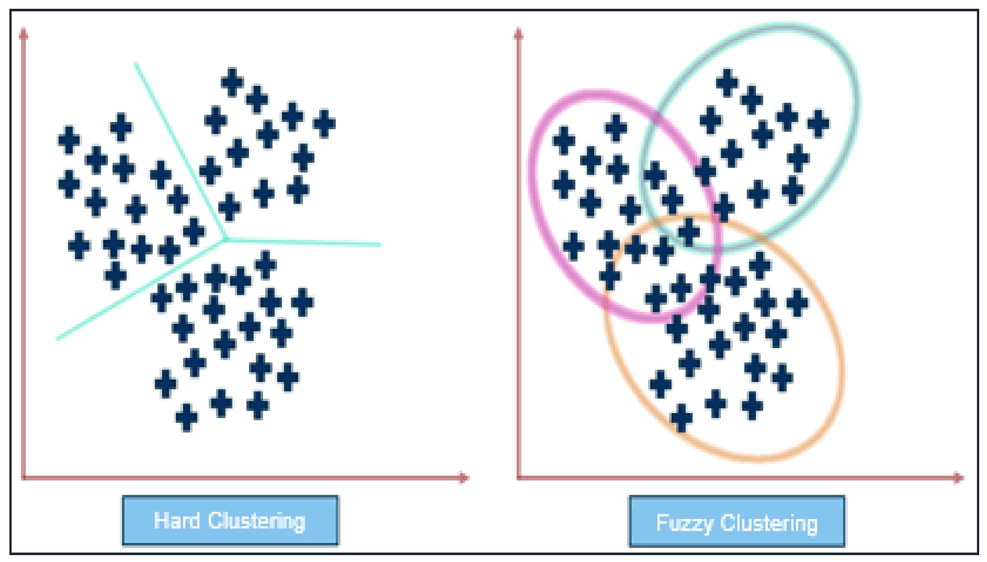
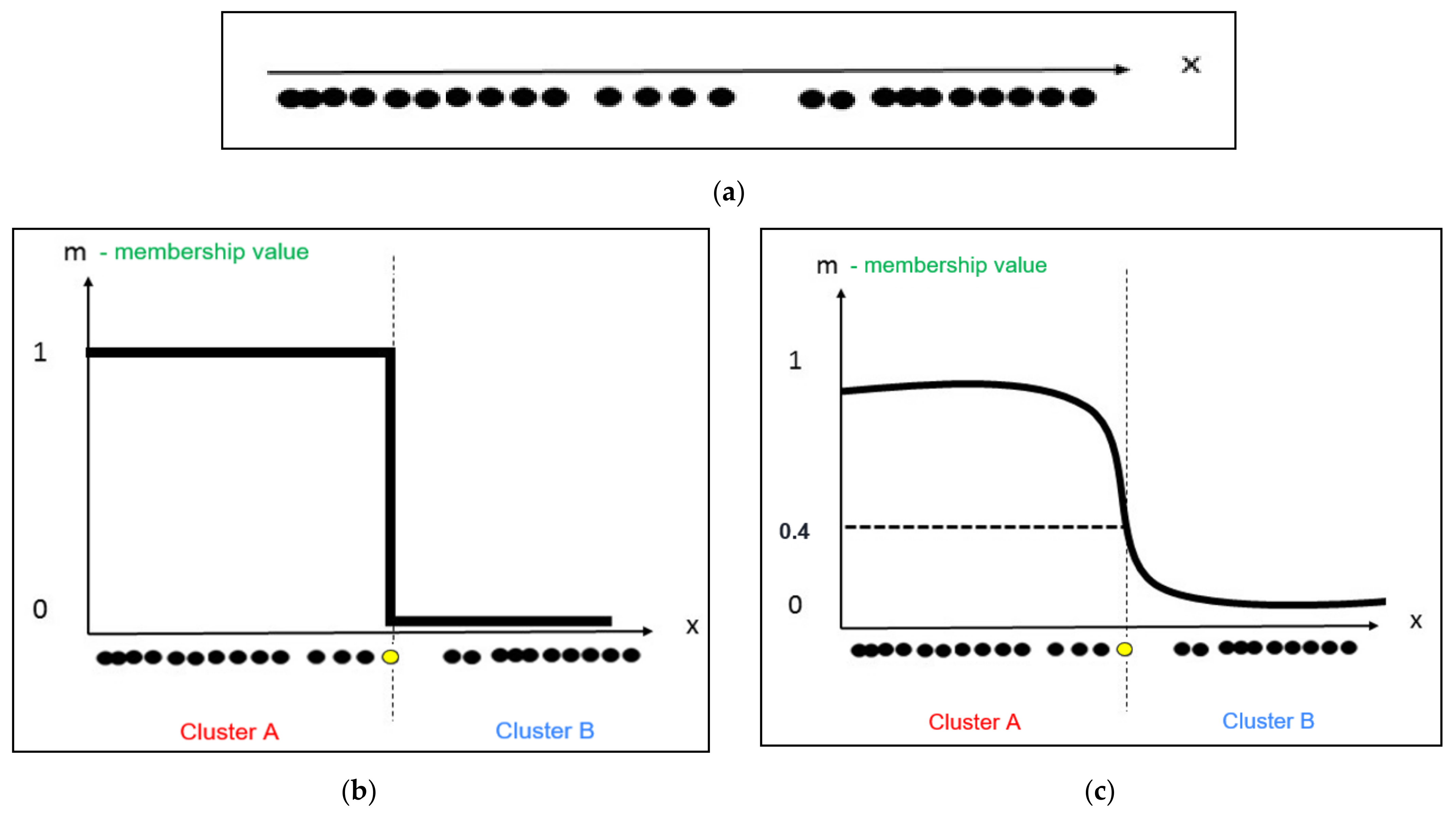
3.4.1. Fuzzy C-Means Clustering

Clustering is one of the machine learning algorithms that come under unsupervised learning and deals with the data structure partition in an unknown area. Clustering is a method that separates data into clusters (groups) by their value. Data under the same cluster must be similar and at the same time must be different from data under other clusters. Clustering algorithms can be designed according to the problems and can be divided into two main groups, traditional and modern. Traditional and modern clustering methods include several types of clustering methods [49].

The traditional clustering algorithms can be divided into nine categories, which mainly contain 26 commonly used ones as follows:

• Clustering algorithm based on partition-k-means, k-medoids, PAM, CLARA, CLARANS
• Clustering algorithm based on hierarchy—BIRCH, CURE, ROCK, chameleon
• Clustering algorithm based on fuzzy theory—FCM, FCS, MM
• Clustering algorithm based on distribution—DBCLASD, GMM
• Clustering algorithm based on density—DBSCAN, OPTICS, Mean-shift
• Clustering algorithm based on graph theory—CLICK, MST
• Clustering algorithm based on grid—STING, CLIQUE
• Clustering algorithm based on fractal theory—FC
• Clustering algorithm based on model—COBWEB, GMM, SOM, ART

The modern clustering algorithms can be divided into 10 categories, which mainly contain 45 commonly used ones as follows:

• Clustering algorithm based on kernel—kernel k-means, kernel SOM, kernel FCM, SVC, MMC, MKC
• Clustering algorithm based on ensemble—methods for generating the set of clusters: 4 types of consensus function: CSPA, HGPA, MCLA, VM, HCE, LAC, WPCK, sCSPA, sMCLA, sHBGPA
• Clustering algorithm based on swarm intelligence—ACO_based (LF), PSO_based, SFLA_based, ABC_based
• Clustering algorithm based on quantum theory—QC, DQC
• Clustering algorithm based on spectral graph theory—SM, NJW
• Clustering algorithm based on affinity propagation—AP
• Clustering algorithm based on density and distance—DD
• Clustering algorithm for spatial data—DBSCAN, STING, Wavecluster, CLARANS
• Clustering algorithm for data stream—STREAM, CluStream, HPStream, DenStream
• Clustering algorithm for large-scale data-k-means—BIRCH, CLARA, CURE, DBSCAN, DENCLUE, Wavecluster, FC

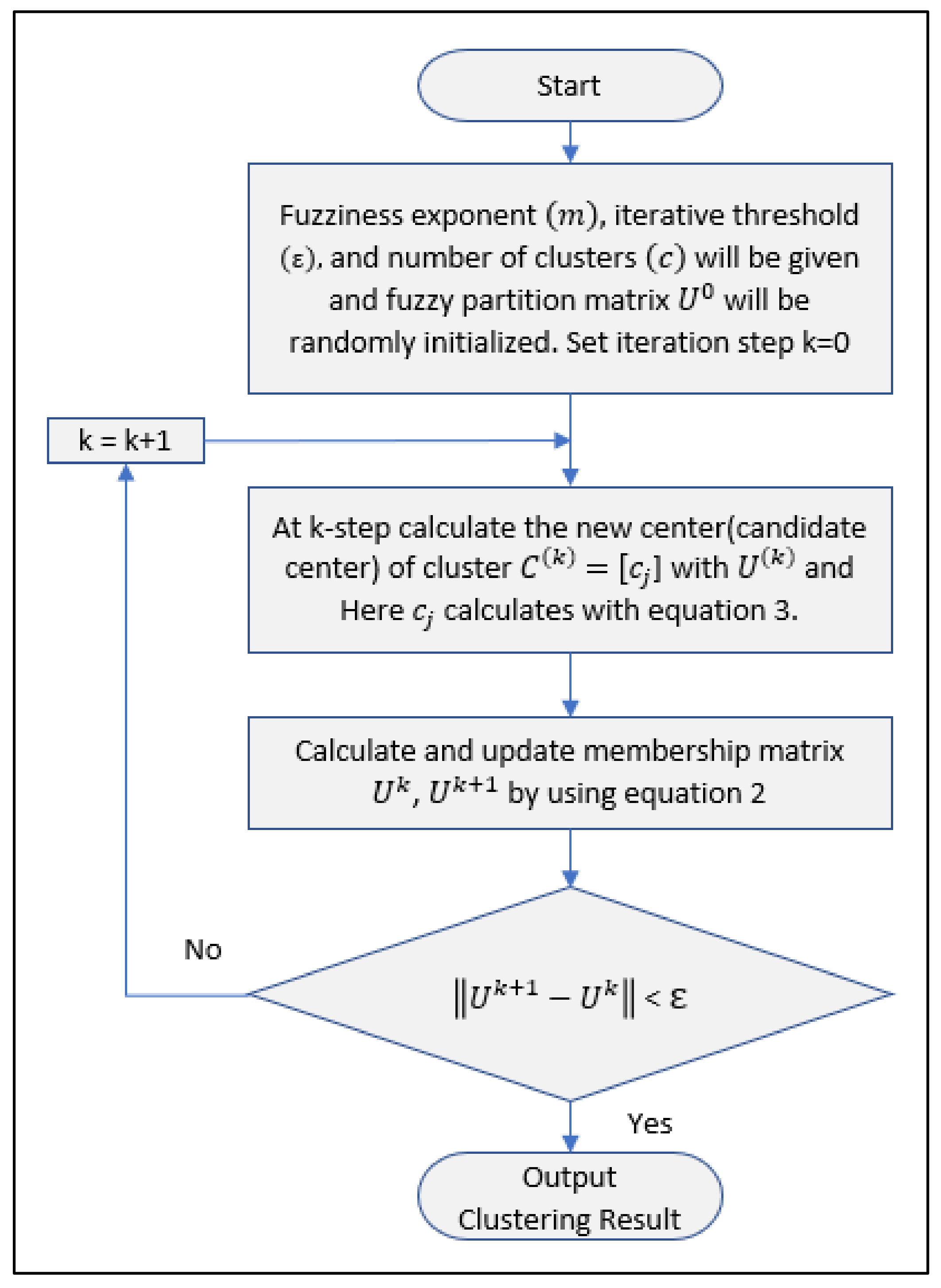
Fuzzy c-means is one of the dominant algorithms, among others. The FCM algorithm is relatively identical to the k-means algorithm, which aims to partition data into k clusters in which each datum belongs to the one cluster with the nearest cluster centroid. K-means is a hard-clustering algorithm originated by MacQueen in 1967 [50]. It assembles data under one cluster only, which leads to the data point being under one cluster or under another. Dissimilar to k-means FCM is a soft clustering algorithm that puts the data under two or more clusters with partition value. This method is expanded by Dunn in 1973 [51] and improved by Bezdek in 1981 [52] and in 1984 [53]. Figure 5 illustrates the difference between hard and soft clustering.

Therefore, in the figure above the results of clustering for both hard (k-means) and soft (c-means) for the same dataset are given, and in the hard clustering, it is clear that data under some clusters cannot be under another one. In soft clustering, overlapped data between two clusters are not clear, given that those overlapped data belong to some cluster. In that case, membership value will decide which cluster the data belong to. Data will be labeled with the cluster from which the data will obtain a higher membership value . To better understand the membership and fuzzy concept, see the one-dimensional dataset given below on an X-axis in Figure 6a [12,54]:

See in the Figure 6b,c below how clustering results will be on both clustering methods according to the membership value of the data points.

The data points can be divided into two clusters. By choosing a threshold on the X-axis, the dataset is separated into two clusters. The output of clustering results is data labeled as ’Cluster A’ and ’Cluster B’, as seen in the above Figure 6b,c. In Figure 6b, each data point belonging to the data set would therefore have a membership coefficient of 0 or 1, even the data point in the middle of the two clusters, which is colored with yellow. This membership coefficient of each corresponding data point is represented by the inclusion of the Y-axis. In Figure 6c, each data point can have membership value to both given clusters. By relaxing the definition of membership coefficients from strictly 0 or 1, these values can range from any value from 0 to 1. As one we can see, the middle data point belongs to Cluster A and Cluster B, with membership values of 0.4 and 0.6, respectively. Therefore, fuzzy logic will be the main difference between k-means and c-means clustering, and membership value decides the cluster of the data points.

The focus of FCM is to minimize the following objective function [53]:

$$J_m={\sum }_{i=1}^N {\sum }_{j=1}^C u_{ij}^m \Vert x_i-c_j{\Vert }^2$$

(1)

where $\left(m\right)$ is the weighting exponent and that is a real number greater than 1, C is the number of clusters, $(u_{ij}$) is the degree of membership of $(x_i$) in the cluster $\left(j\right)$, $(x_i$) is the $\left(i\right)th$ of d-dimensional data, $(c_j$) is the d-dimensional center of the cluster, and ‖*‖ is any norm expressing the similarity between any measured data and the center. The variable $\left( u_{ij}^m\right)$ is defined as follows:

$$u_{ij}^m=\frac{1}{{{\displaystyle \sum }}_{k=1}^C{(\frac{\Vert x_i-c_j\Vert }{\Vert x_i-c_k\Vert })}^{\frac{2}{m-1}}}$$

(2)

Cluster centers $(c_j$) is defined as follows:

$$c_j=\frac{{{\displaystyle \sum }}_{i=1}^N u_{ij}^m\ast x_i}{{{\displaystyle \sum }}_{i=1}^N u_{ij}^m}$$

(3)

This iteration stops when $ma{x}_{ij}\left\{\Vert u_{ij}^{\left(k+1\right)}- u_{ij}^{\left(k\right)}\Vert \right\}$ < ε, where ε is a termination criterion between 0 and 1, and where $(k$) is the iteration steps. This procedure calculates a local minimum or a saddle point of $J_m$.

Solution of the object function $J_m$ can be obtained by following steps:

Step 1. 

Set values for c (number of clusters), m (fuzziness exponent), ε

Step 2. 

Initialize fuzzy partition matrix $\mathit{U}=\left[{\mathit{u}}_{\mathit{i}\mathit{j}}\right], {\mathit{U}}^{\left(\mathbf{0}\right)}$

Step 3. 

At k-step: calculate the c cluster centers(centroids) ${\mathit{C}}^{\left(\mathit{k}\right)}=\left[{\mathit{c}}_{\mathit{j}}\right]$ with ${\mathit{U}}^{\left(\mathit{k}\right)}$. Where ${\mathit{c}}_{\mathit{j}}$ calculates with Equation (3)

Step 4. 

Calculate and update membership matrix ${\mathit{U}}^{\left(\mathit{k}\right)}, {\mathit{U}}^{\left(\mathit{k}+\mathbf{1}\right)}$. Equation (2)

Step 5. 

If $\mathit{max}\left\{\Vert {\mathit{U}}^{\left(\mathit{k}+\mathbf{1}\right)}-{\mathit{U}}^{\left(\mathit{k}\right)}\Vert \right\}$ < ε then stop, otherwise set k = k+1 and return to Step 3

See the flow chart diagram of the algorithm below in Figure 7.

A number of clusters $c$ can be calculated with several methods such as the elbow [55,56] or fuzzy partition coefficient (FPC). In this work, we implemented FPC. FPC uses fuzzy partition matrices to measure the degree of fuzziness of the final partitioned cluster, and the largest value is the better partition results. FPCs are defined in the range of 0 to 1, and 1 is the best. The following section describes how FCM implemented this task and how data have been trained.

3.4.2. Experiment Parameters and Environment

In order to implement the FCM algorithm, there are parameters such as number of clusters ($c$), fuzziness exponent ($m$), and ($\epsilon$) iterative threshold (smallest positive constant) that we have to set beforehand. As we mentioned above for the number of clusters, we used FPC, and according to the experiment number of clusters in the blocks, we mostly used 2 and 3 and rarely 4 and 5. As the threshold value, we set 0.005 in the experiment. The value of the fuzziness component m we set as m = 2.

Environment setting for the experiment:

• OS: Windows 10 Pro
• Processor: Intel(R) Core (TM) i7-10700 CPU @2.90 GHz
• RAM: 32 GB
• System Type: 64 bit
• Platform: Jupyter Notebook (Python)

3.4.3. Data Training Method

Data trained in this work are gathered by several vessels that have SONAR sensors installed on their board and that crowdsource data collected in the southern part of South Korea. Figure 8 [57] below indicates that the red marked area in the map is the area of experimental data of this work. The trained area latitude is between 35.00 to 35.25, and longitude is between 128.75 to 129.25, and that is approximately 27.8 to 45.4 km.

The data that vessels have been collecting and sending to our server have been stored as in

Table 2. Example of data for the training.

Device_id	Time	Latitude	Longitude	Depth
SY-T02	2020-02-27 11:19:03	35.0001678466797	128.919357299805	14.5 m
SY-T02	2020-02-28 10:10:28	35.0003662109375	128.919677734375	14.5 m
SY-T04	2019-08-27 09:50:45	35.0004158020020	128.919662475586	26.4 m
SY-T05	2019-02-27 08:19:08	35.0001335144043	128.919326782227	26.5 m
SY-T02	2019-01-21 12:11:50	35.0006332397461	128.919570922852	25.5 m
SY-T04	2018-09-23 07:23:07	35.0006484985352	128.919067382812	9.8 m
SY-T03	2020-04-21 13:11:50	35.0006332397461	128.919570922852	25.7 m
SY-T04	2021-01-10 17:13:09	35.0006484985352	128.919067382812	10.2 m

below.

As the table illustrates, device, id, time, location (latitude, longitude), and depth are collected by sensors and stored in the database. There are also additional data such as water temperature, speed of the wind, direction of the wind, speed of ships, and so on. However, for the training of this work, it is enough to have depth and location information. The training area is immense enough, and of course, the depth of one place in the ocean makes diversity from the depth of another place. Moreover, at the same time, the depth of the sea does not switch radically in a long-distance like 10 to 100 m. Because of that reason, we cannot cluster all data under the same measurement, and it is impossible to cluster data by only one single point in the map. The explanation is a number of data in one point almost equal to 1. Therefore, before the experiment with all data, we divided the whole experimental area into blocks (small size area). Each divided block is approximately 100 by 100 m, and we implemented FCM to each block, see Figure 9 below.

There are roughly 6,384,000 data points in the dataset, and after segregating them into blocks, 125,000 training blocks appear in the training area.

The following procedure is needed in order to implement the FCM algorithm for any crowdsourced bathymetry data by using our methodology:

• Define minimum and maximum coordinates (latitude, longitude).
• Divide the whole training zone into the blocks. The approximate size of the blocks should be 100 to 100 m.
• Sort blocks that have more than 200 data points. If there are fewer data points in the blocks, no use of FCM in that block.
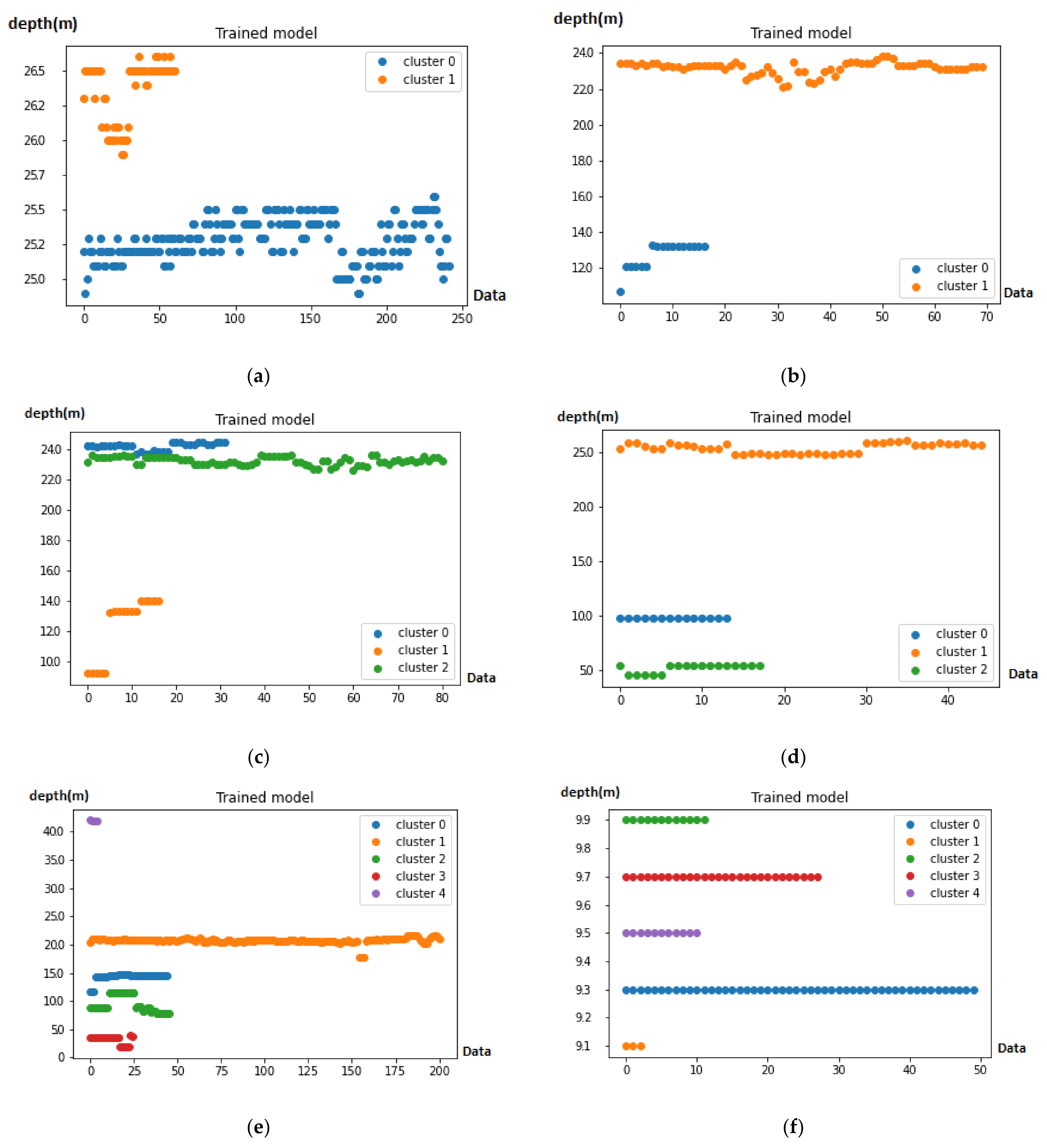
• Implement FCM to each block.
• Compare with real data.

To validate the level of accuracy of the results, we calculated mean absolute error by utilizing Equation (4) below and compared S-57 Electronic Navigation Charts (ENC) data, which are measured by the Korean National Oceanographic Agency, with our results.

$$MeanAbsoluteError=\frac{1}{\mathrm{N}}{\sum }_{i=1}^N \Vert y_i-\widehat{y_i}\Vert$$

(4)

where $N$ is the number of data, $y_i$ is real data, $\widehat{y_i}$ is predicted data.

4. Results

Having trained the dataset by separating the training area into blocks, we obtained the expected clustering results. According to the results, the number of clusters in most of the blocks is equal to 2 or 3. Furthermore, there are numerous clusters such as more than 5, but in that case, we may encounter the identical diversity between each data points in the block.

As highlighted in Figure 10 below, the clustering results and the number of clusters in the trained blocks contrast; nonetheless, if data points are enough, then clustering results are also clear enough.

After training each block, we obtained results including the depth of data points, the numbers of data points in the clusters, and the label that determines which data belong to which cluster. Figure 10a,b are patterns of two clusters in a block. Having obtained the data with their cluster number, we had selected the major cluster that is able to represent the predicted value of that block. In order to choose the phenomenal cluster among other clusters, we just used counting the data under all clusters, and whichever cluster possesses more data becomes the main cluster of that block. As a result, the average value of the main cluster will be the value of the block. In Figure 10a, blue-colored dots are the main cluster, and orange ones can be labeled as slightly inaccurate data because of the wave in the sea surface. Figure 10b is also an example of two clusters in a block, but here orange dots are the main cluster and blue is the cluster of incorrect data that could be improper owing to the obstacles in the water. Figure 10c,d are examples of three clusters in a block: (c) indicates green is the premium cluster of the block, blue is a cluster that indicates the value of the points is very close to the main cluster but incorrect because of the wave, and orange is totally incorrect data that are gained after encountering obstacles. In (d), orange is the main data that the average value of cluster is around 25 m, blue is around 10 m, and green is approximately 5 m are all wrong data that are measured improperly because of an obstacle. In Figure 10e,f, nearly the same situations can also be seen, such as one dominated cluster and the four clusters with the wrong data. Those figures highlight the examples of five clusters in one block.

It is certain that the failures can also be observed through the proposed method. On the other hand, in the blocks where the errors occur, only wrong data were collected by a vessel, which means the number of data close to the actual data is drastically less than or completely absent relative to the number of erroneous data. For instance, as shown in Figure 11a,b, main clusters are presented as orange (in a) and blue (in b), and the values given to the blocks after clustering are 5.8 and 6.3 m, respectively, while the real data of the blocks that are measured by the Korean Agency are 41 and 43 m, respectively.

In those kinds of cases, the investigations show an error that occurs only in the blocks that only collected less and wrong data from practically all the crowd. This indicates that there is a lot of failing in data collection, not only in the proposed data sorting model. In the forthcoming works, we intend to draw attention to eliminating such shortcomings through double-level clustering.

In the study area, we made a comparison of our results with the data taken from the Korean National Oceanographic Agency S-57 ENC. The accuracy of the proposed model was measured by calculating the mean absolute error of real data and mean value of each block and calculating the mean absolute error of real data and FCM clustering data. See

Table 3. Comparison of mean value and fuzzy c-means value of each block.

	By Mean Value of Each Block	By FCM Value of Each Block
Mean Absolute Error	2.09 m	1.67 m

below.

The table illustrates comparison results of the mean absolute error between mean values of each block of real data (S-57 ENC) and fuzzy values of each block of our method result. The experiment results show the mean absolute error of our method is equal to approximately 1.67 m, and it is smaller than the mean absolute error of real data (S-57 ENC), 2.09 m.

5. Conclusions and Future Work

Machine learning approaches have been used in addressing challenges in many spheres, and the methods of ML are also widely used in classification and prediction problems. An unsupervised learning model proposed in this work is aimed to predict the depth of seawater by enhancing the accuracy of data, which is measured by crowdsourced echo soundings. According to the results, the proposed method to predict the depth by applying FCM clustering can be implemented in the current problem and provide superior results. The failed cases prove that crowdsourced data may include only failed data, and they show that by improving data collection, the accuracy of our prediction model can be increased. The concluding result, which is a comparison of our model result with real data collected by Korean National Oceanographic Agency S-57 ENC, indicates that even if we have blocks with only failed data, our model is more productive compared to the normal average value. The mean absolute error of two cases, our model result, 1.67 m, and average value, 2.09 m, can prove the efficiency of the work. In the upcoming studies, we aim to focus on advancing our proposed model and handling the above failed cases by two-step clustering excluding the real data.

References

1. Kamolov, A.; Park, S.H. An IoT Based Smart Berthing (Parking) System for Vessels and Ports. In ICMWT 2018: Mobile and Wireless Technology 2018; Kim, K., Kim, H., Eds.; Lecture Notes in Electrical Engineering; Springer: Singapore, 2019; Volume 513. [Google Scholar]
2. Kamolov, A.; Al-Absi, M.A.; Lee, H.J.; Park, S.H. Smart Flying Umbrella Drone on Internet of Things: AVUS. In Proceedings of the 21st International Conference on Advanced Communication Technology (ICACT), PyeongChang, Korea, 17–20 February 2019. [Google Scholar]
3. Hyundai Heavy Industries Debuts ‘Smart Ship’ Solution. Available online: https://www.marinelink.com/news/industries-solution427522 (accessed on 9 February 2021).
4. Japan Develops Smart Ship Platform. Available online: https://www.rivieramm.com/opinion/opinion/japan-develops-smart-ship-platform-31339 (accessed on 10 February 2021).
5. We4Sea—Efficiency Solutions for Ships. Available online: https://www.we4sea.com/ (accessed on 10 February 2021).
6. Hamburg Port—Interactive port map of the Port of Hamburg. Available online: https://www.hafen-hamburg.de/en/portmap (accessed on 10 February 2021).
7. Amsterdam Port. Available online: https://www.portofamsterdam.com/en/shipping/arrivals-and-departures (accessed on 10 February 2021).
8. Kamolov, A.; Park, S. An IoT-Based Ship Berthing Method Using a Set of Ultrasonic Sensors. Sensors 2019, 19, 5181. [Google Scholar] [CrossRef] [PubMed] [Green Version]
9. Kamolov, A.; Park, S.H. IoT based smart reporting and mooring system for vessels. In Proceedings of the Korean Institute of Information and Communication Sciences Conference, Chungcheongnam-do, Korea, 10 October 2017; Volume 21, pp. 0395–0398. [Google Scholar]
10. Geertsma, R.D.; Negenborn, R.R.; Visser, K.; Hopman, J.J. Design and control of hybrid power and propulsion systems for smart ships: A review of developments. Appl. Energy 2017, 194, 30–54. [Google Scholar] [CrossRef]
11. Mapping the Ocean Floor by 2030. Available online: https://www.gislounge.com/mapping-the-ocean-floor-by-2030/ (accessed on 11 February 2021).
12. Fuzzy Clustering. Available online: https://en.wikipedia.org/wiki/Fuzzy_clustering (accessed on 14 December 2020).
13. Wölfl, A.-C.; Snaith, H.; Amirebrahimi, S.; Devey, C.W.; Dorschel, B.; Ferrini, V.; Huvenne, V.A.I.; Jakobsson, M.; Jencks, J.; Johnston, G.; et al. Seafloor Mapping—The Challenge of a Truly Global Ocean Bathymetry. Front. Mar. Sci. 2019, 6, 283. [Google Scholar] [CrossRef]
14. Sagawa, T.; Yamashita, Y.; Okumura, T.; Yamanokuchi, T. Satellite Derived Bathymetry Using Machine Learning and Multi-Temporal Satellite Images. Remote Sens. 2019, 11, 1155. [Google Scholar] [CrossRef] [Green Version]
15. Caballero, I.; Stumpf, R.P.; Meredith, A. Preliminary Assessment of Turbidity and Chlorophyll Impact on Bathymetry Derived from Sentinel-2A and Sentinel-3A Satellites in South Florida. Remote Sens. 2019, 11, 645. [Google Scholar] [CrossRef] [Green Version]
16. Salameh, E.; Frappart, F.; Almar, R.; Baptista, P.; Heygster, G.; Lubac, B.; Raucoules, D.; Almeida, L.P.; Bergsma, E.W.J.; Capo, S.; et al. Monitoring Beach Topography and Nearshore Bathymetry Using Spaceborne Remote Sensing: A Review. Remote Sens. 2019, 11, 2212. [Google Scholar] [CrossRef] [Green Version]
17. Su, H.; Liu, H.; Wu, Q. Prediction of Water Depth from Multispectral Satellite Imagery—The Regression Kriging Alternative. IEEE Geosci. Remote Sens. Lett. 2015, 12, 2511–2515. [Google Scholar]
18. Lyzenga, D.R. Passive remote-sensing techniques for mapping water depth and Bottom Features. Appl. Opt. 1978, 17, 379–383. [Google Scholar] [CrossRef]
19. Lyzenga, D.R.; Malinas, N.P.; Tanis, F.J. Multispectral bathymetry using a simple physically based algorithm. IEEE Trans. Geosci. Remote Sens. 2006, 44, 2251–2258. [Google Scholar] [CrossRef]
20. Kao, H.-M.; Ren, H.; Lee, C.-S.; Chang, C.-P.; Yen, J.-Y.; Lin, T.-H. Determination of shallow water depth using optical satellite images. Int. J. Remote Sens. 2009, 30, 6241–6260. [Google Scholar] [CrossRef]
21. Dekker, A.G.; Phinn, S.R.; Anstee, J.; Bissett, P.; Brando, V.E.; Casey, B.; Fearns, P.; Hedley, J.; Klonowski, W.; Lee, Z.P.; et al. Intercomparison of shallow water bathymetry, hydro-optics, and benthos mapping techniques in Australian and Caribbean coastal environments: Intercomparison of shallow water mapping methods. Limnol. Oceanogr.-Meth. 2011, 9, 396–425. [Google Scholar] [CrossRef] [Green Version]
22. Kanno, A.; Tanaka, Y.; Kurosawa, A.; Sekine, M. Generalized Lyzenga’s predictor of shallow water depth for multispectral satellite imagery. Mar. Geod. 2013, 36, 365–376. [Google Scholar] [CrossRef] [Green Version]
23. Manessa, M.D.M.; Kanno, A.; Sekine, M.; Haidar, M.; Yamamoto, K.; Imai, T.; Higuchi, T. Satellite-derived bathymetry using random forest algorithm and worldview-2 Imagery. Geoplanning J. Geomat. Plan. 2016, 3, 117–126. [Google Scholar] [CrossRef] [Green Version]
24. Traganos, D.; Poursanidis, D.; Aggarwal, B.; Chrysoulakis, N.; Reinartz, P. Estimating Satellite-Derived Bathymetry (SDB) with the Google Earth Engine and Sentinel-2. Remote Sens. 2018, 10, 859. [Google Scholar] [CrossRef] [Green Version]
25. Mavraeidopoulos, A.K.; Pallikaris, A.; Oikonomou, E. Satellite Derived Bathymetry (SDB) and Safety of Navigation. Int. Hydrogr. Rev. 2017, 17, 7–20. [Google Scholar]
26. Banic, J.; Sizgoric, S. Scanning Lidar bathymeter for water depth measurement. Laser Radar Technol. Appl. 1986, 187–195. [Google Scholar] [CrossRef]
27. Wilson, N.; Parrish, C.E.; Battista, T. Mapping Seafloor Relative Reflectance and Assessing Coral Reef Morphology with EAARL-B Topobathymetric Lidar Waveforms. Estuaries Coasts 2019, 1–15. [Google Scholar] [CrossRef] [Green Version]
28. Irish, J.L.; White, T.E. Coastal engineering applications of high-resolution LiDAR bathymetry. Coast. Eng. 1998, 35, 47–71. [Google Scholar] [CrossRef]
29. Wang, C.; Li, Q.; Liu, Y.; Wu, G.; Liu, P.; Ding, X. A comparison of waveform processing algorithms for single-wavelength LiDAR bathymetry. ISPRS J. Photogramm. Remote Sens. 2015, 101, 22–35. [Google Scholar] [CrossRef]
30. Bincai, C.; Yong, F.; Li, G.; Haiyan, H.; Zhengzhi, J.; Bijiao, S.; Lele, L. An active-passive fusion strategy and accuracy evaluation for shallow water bathymetry based on ICESat-2 ATLAS laser point cloud and satellite remote sensing imagery. Int. J. Remote Sens. 2021, 42, 2783–2806. [Google Scholar]
31. Lyzenga, D.R. Shallow-water bathymetry using combined Lidar and passive multispectral scanner data. Int. J. Remote Sens. 1985, 6, 115–125. [Google Scholar] [CrossRef]
32. Saylam, K.; Brown, R.A.; Hupp, J.R. Assessment of depth and turbidity with airborne Lidar bathymetry and multiband satellite imagery in shallow water bodies of the Alaskan North Slope. Int. J. Appl. Earth Obs. Geoinf. 2017, 58, 191–200. [Google Scholar] [CrossRef]
33. Ma, Y.; Xu, N.; Liu, Z.; Yang, B.; Yang, F.; Wang, X.H.; Li, S. Satellite-derived bathymetry using the ICESat-2 lidar and Sentinel-2 imagery datasets. Remote Sens. Environ. 2020, 250, 112047. [Google Scholar] [CrossRef]
34. Pike, S.; Traganos, D.; Poursanidis, D.; Williams, J.; Medcalf, K.; Reinartz, P.; Chrysoulakis, N. Leveraging Commercial High-Resolution Multispectral Satellite and Multibeam Sonar Data to Estimate Bathymetry: The Case Study of the Caribbean Sea. Remote Sens. 2019, 11, 1830. [Google Scholar] [CrossRef] [Green Version]
35. Tian, J.; Li, C.; Liu, J.; Yu, F.; Cheng, S.; Zhao, N.; Wan Jaafar, W.Z. Groundwater Depth Prediction Using Data-Driven Models with the Assistance of Gamma Test. Sustainability 2016, 8, 1076. [Google Scholar] [CrossRef] [Green Version]
36. Yang, F.; Qiao, Y.; Wei, W.; Wang, X.; Wan, D.; Damaševičius, R.; Woźniak, M. DDTree. A Hybrid Deep Learning Model for Real-Time Waterway Depth Prediction and Smart Navigation. Appl. Sci. 2020, 10, 2770. [Google Scholar] [CrossRef] [Green Version]
37. Kang, C. A Differential Dynamic Positioning Algorithm Based on GPS/Beidou. Procedia Eng. 2016, 137, 590–598. [Google Scholar] [CrossRef]
38. Shiri, J. Wavelet and neuro-fuzzy conjunction model for predicting water table depth fluctuations. Hydrol. Res. 2012, 43, 286–300. [Google Scholar]
39. Vodas, M.; Pelekis, N.; Theodoridis, Y.; Ray, C.; Karkaletsis, V.; Petridis, S.; Miliou, A. Efficient AIS Data Processing for Environmentally Safe Shipping. Spoud. J. Econ. Bus. 2014, 63, 181–190. [Google Scholar]
40. Li, S.; Chen, X.; Chen, L.; Chen, L.; Zhao, Y.; Sheng, T.; Bai, Y. Data Reception Analysis of the AIS on board the TianTuo-3 Satellite. J. Navig. 2017, 70, 761–774. [Google Scholar] [CrossRef]
41. Yang, D.; Wu, L.; Wang, S.; Jia, H.; Li, K.X. How big data enriches maritime research–a critical review of automatic identification system (AIS) data applications. Transp. Rev. 2019, 39, 755–773. [Google Scholar] [CrossRef]
42. How is Sound Used to Measure Water Depth? Available online: https://dosits.org/people-and-sound/navigation/how-is-sound-used-to-measure-water-depth/ (accessed on 12 February 2021).
43. Sea Floor Mapping. Available online: https://oceanexplorer.noaa.gov/explorations/lewis_clark01/background/seafloormapping/seafloormapping.html (accessed on 11 February 2021).
44. Depth Sounding Techniques That Preceded the Modern Day SONAR Technology. Available online: https://www.thevintagenews.com/2017/02/23/depth-sounding-techniques-that-preceded-the-modern-day-sonar-technology/ (accessed on 13 February 2021).
45. How is Sound Used to Map the Seafloor? Available online: https://dosits.org/people-and-sound/examine-the-earth/map-the-sea-floor/ (accessed on 14 February 2021).
46. Eakins, B.W.; Sharman, G.F. Volumes of the World’s Oceans from ETOPO2v2; NOAA National Geophysical Data Center: Boulder, CO, USA, 2010. [Google Scholar]
47. Mao, K.; Capra, L.; Harman, M.; Jia, Y. A Survey of the Use of Crowdsourcing in Software Engineering. J. Syst. Softw. 2017, 126, 57–84. [Google Scholar] [CrossRef] [Green Version]
48. Pavić, I.; Mišković, J.; Kasum, J.; Alujević, D. Analysis of Crowdsourced Bathymetry Concept and It’s Potential Implications on Safety of Navigation. TransnavInt. J. Mar. Navig. Saf. Sea Transp. 2020, 14, 681–686. [Google Scholar] [CrossRef]
49. Xu, D.; Tian, Y. A comprehensive survey of clustering algorithms. Ann. Data Sci. 2015, 2, 165–193. [Google Scholar] [CrossRef] [Green Version]
50. MacQUEEN, J.B. Some Methods for Classification and Analysis of Multivariate Observations. In Proceedings of the Fifth Berkeley Symposium on Mathematical Statistics and Probability: Weather Modification; Lucien, M., Le, C., Jerzy, N., Eds.; University of California Press: Berkeley/Los Angeles, CA, USA, 1967; Volume 1, pp. 281–297. [Google Scholar]
51. Dunn, J.C. A Fuzzy Relative of the ISODATA Process and Its Use in Detecting Compact Well-Separated Clusters. J. Cybern. 1973, 3, 32–57. [Google Scholar] [CrossRef]
52. Bezdek, J.C. Objective function clustering. In Pattern Recognition with Fuzzy Objective Function Algorithms, 1st ed.; Springer Inc.: Secaucus, NJ, USA, 1981; pp. 43–93. ISBN 978-1-4757-0452-5. [Google Scholar]
53. Bezdek, J.C.; Ehrlich, R.; Full, W. FCM: The fuzzy c-means clustering algorithm. Comput. Geosci. 1984, 10, 191–203. [Google Scholar] [CrossRef]
54. Fuzzy C-Means Clustering. Available online: https://matteucci.faculty.polimi.it/Clustering/tutorial_html/cmeans.html (accessed on 10 December 2020).
55. Kodinariya, T.M.; Makwana, P.R. Review on determining number of Cluster in K-Means Clustering. Int. J. Adv. Res. Comput. Sci. Manag. Stud. 2013, 1, 2321–7782. [Google Scholar]
56. Bholowalia, P.; Kumar, A. EBK-Means: A Clustering Technique based on Elbow Method and K-Means in WSN. Int. J. Comput. Appl. 2014, 105, 17–24. [Google Scholar]
57. Choi, K. Electronic Navigation Chart Standards and Viewers. Available online: https://www.slideshare.net/KyusungChoi/ss-72798127 (accessed on 20 May 2021).
Figure 1. The first printed map of ocean depths with information provided from the USS Dolphin (1853).
Sustainability 13 05823 g001
Figure 2. Measuring of depth of ocean by SONAR.
Sustainability 13 05823 g002
Figure 3. Crowdsourced bathymetry.
Sustainability 13 05823 g003
Figure 4. Example of measuring of same seabed: (a) accurate measuring; (b) inaccurate measuring when there is an obstacle while measuring; (c) inaccurate measuring when there is a strong wave in sea surface.
Sustainability 13 05823 g004
Figure 5. Hard and soft (fuzzy) clustering.
Sustainability 13 05823 g005
Figure 6. (a) One-dimensional dataset, (b) membership value of k-means, (c) membership value of FCM.
Sustainability 13 05823 g006
Figure 7. Fuzzy C-mean flow chart diagram.
Sustainability 13 05823 g007
Figure 8. Experiment area in the map.
Sustainability 13 05823 g008
Figure 9. Data training zone.
Sustainability 13 05823 g009
Figure 10. Example of 2, 3, and 5 clustering results. (a) and (b) are examples of two cluster results; (c) and (d) are examples of three cluster results; (e) and (f) are examples of five cluster results.
Sustainability 13 05823 g010
Figure 11. Example of clustering of blocks that has less or no real data. (a) The value of the clustering result is 5.8 m. (b) The value of the clustering result is 6.3 (m).
Sustainability 13 05823 g011