Abstract
This paper presents the seismic analytic fragility curve of soil nail wall structures. The numerical modeling procedure of the soil nail wall is presented and discussed in detail. Nonlinear elements have been used to provide an accurate finite element modeling of the soil nail wall. The effect of different soil modeling approaches is studied. Detailed procedures to select an efficient intensity measure are presented. Analytical fragility curves for the different performance levels of the soil nail wall are developed. Detailed techniques have been used to generate accurate soil modeling, such as the Mohr-Coulomb model (MC), Hardening Soil model (HS), and Hardening Soil model with Stiffness effect from small strains (HSS), and these are studied. Incremental dynamic analysis (IDA) is implemented to capture the response of the wall from linear to nonlinear levels. The efficiency of the two common intensity measures is studied (PGA and Sa(T1,5%)). It has been demonstrated that HSS and HS models are more reliable techniques for soil modeling. Two common intensity measures are studied, and the efficiency and the sufficiency of them are compared. It has been suggested that Sa(T1,5%) is a more efficient intensity measure than PGA for soil nail structures due to less depression in the IDA results. Different performance levels were defined to develop analytical fragility curves for different damage states.
1. Introduction
Seismic vulnerability and seismic performance of structures are becoming an important subject, especially after the 1971 San Fernando earthquake because of damages during the large excitations. In the soil-nailed walls, the structures are constructed for long-term and short-term service life and experience different loading conditions. Fragility curves are a mathematical tool to provide a relationship between the earthquake intensities and the probability of reaching the target damage state. Fragility curves are generated using two approaches: empirical and analytical. In the first approach, fragility curves are developed empirically by evaluation of the historical data from the historical earthquakes, and in the second one, they are generated by applying nonlinear dynamic analyses to the structure models under a large number of ground motions. In empirical fragility curves, a vast volume of damage information is needed for the selected class of structure, and this is one of the drawbacks of this method. The analytical fragility curve can be used for structures that did not experience an earthquake. Basoz and Kiremidjian [1] researched generating empirical fragility curves for California highway bridges. Shinozuka et al. [2] and Yamazaki et al. [3] provided empirical fragility curves by considering the actual damage data observed from the Kobe earthquake. Shinozuka et al. [2] studied the usage of a nonlinear static procedure to develop the fragility of the structure, but they indicated that this method doesn’t show reasonable agreement in predicting all levels of damage with nonlinear time history analysis. Many other scientists have studied the PSDA of structures [4,5,6,7].
Analytical fragility curves are developed using two methods: the scaling method and the cloud method. In the scaling approach, all the earthquake ground motions need to be scaled to a selective intensity measure, and IDA is applied at different levels and steps of intensity measure. In the cloud method, us-scaled earthquake records are used in time history analysis.
Developing analytical fragility curves based on the probabilistic seismic demand model (PSDM) framework was first proposed by Shome et al. [8]. They formulated the PSDM to consider the uncertainty of the seismic hazard with a nonlinear analysis of structural response. A PSDM presents the conditional probability of the soil nail wall structure (i.e., wall displacement) reaching a certain damage state (DS) for a given earthquake intensity measure (IM) level, as demonstrated in Equation (1) [8]:
An essential task in PSDM is to reduce the uncertainties related to the earthquake intensity measure by selecting an appropriate earthquake IM. Researchers have investigated IM selection for structures. The Applied Technology Council [9] selected the Modified Mercalli Intensity Scale. FEMA’s Hazus program [10] (Geographic information system-based natural hazard analysis tool) used peak ground acceleration (PGA) and peak ground displacement (PGD) [10].
Shome et al. [11] proposed the elastic spectrum at the fundamental period of the structure Sa (T) as a measure of earthquake intensity. Tothong and Luco et al. [12] considered displacement spectra Sd (T) as an alternative IM for structures. Padgett et al. [13] studied different intensity measure highway bridge portfolios and proposed PGA as an appropriate IM. Bayat et al. [14] proposed the average value of the Sa (between a lower and upper structural period), called Averaged Spectral Acceleration (ASA), for highway bridges. Aside from these common IMs, more complex parameters or vector-based IMs have been studied by past researchers for structures [15,16,17,18,19,20,21]. Since the structural response and behavior of the structure are different, it is not reasonable to propose one intensity measure for a wide range of the structures (bridges, buildings, soil nailed wall, etc.). Therefore, there is a substantial need to extend the PSDM for a specific class of structures in terms of IM selection. To our knowledge, there is no work on the IM selection of soil-nailed wall structures. This study extends the effort on IM selection for soil nail wall structures to reduce earthquake uncertainty and develop much more reliable fragility curves. The first attempt has been made on common IMs, such as PGA and Sa(T1,5%), which are widely used.
Incremental dynamic analysis is implemented to achieve seismic fragility curves for the soil nail walls. Developing analytical fragility curves requires a combination of earthquake simulation and structural response. The response of the structure is obtained by applying incremental dynamic analysis, which is a reliable method. One of the main objectives of this paper is to assess the vulnerability of soil nail eight meters in height when experiencing different earthquake levels. A detailed finite element model of the wall has been generated, and its seismic analytical fragility curves are developed based on the results of the IDA using a finite element (FE) package, PlAXIS.V8.3.
A Bayesian regression-based demand model with a linear regression formulation in the logarithmic space is developed to predict the maximum displacement for the soil nail wall and the efficiency of the Intensity Measures (IMs). PGA and Sa(T1,5%) are chosen as an intensity measure (IM), and displacement of the wall is chosen as an engineering demand parameter (EDP). The different performance levels of the bridge are considered through slight, moderate, and extensive levels. Bayesian regression analysis has been utilized to develop a probabilistic demand model to predict damage in the soil nail wall. One of the advantages of the Bayesian regression is that uncertainty related to incomplete sample populations is directly considered by standard deviation σ and regression coefficients, which are random variables, rather than constant variables. In another step to propose a suitable intensity measure, the sufficiency of the intensity measures is also examined for the efficient intensity measure. In the end, fragility curves are presented to define the failure probability of the soil nail wall structure.
2. Numerical Modeling and Verification
2.1. Numerical Modeling
PlAXIS.V8.3 finite element software is used to perform site response analysis. Plane strain finite element analyses were used in this program software. Three different soil modeling approaches were used, including MC, HS, and HSS. Table 1 and Table 2 show the detailed soil modeling properties for the verified model and the current study. The plate element is used to model the nail and the shotcrete. Table 2 and Table 3 show the soil nail wall and shield properties. The experimental results indicated that the ratio of soil-cement adhesion over soil cohesion is in a range of 0.85–1.18, and the interface friction angle ratio over soil friction angle ) is in a range of 0.95–1.07. The ratios of and are considered 0.8 [18,19].

Table 1.
Soil, nail, and wall-facing properties were used in the CLOUTERRE project and FE modeling [4].
Table 2.
Geometrical characteristics and other parameters of the nailed walls.
Table 3.
Geotechnical parameters of the behavioral models.
The interface strength reduction factor for shield modeling and soil interaction is also considered as 0.65. Figure 1 represents the modeled wall, along with its dimensions and boundary conditions. 15-node triangular elements were implemented in all simulations. Table 2 tabulated the soil nail wall’s important parameters. The arrangement of the nails is shown in Table 2. The length and distance of the nails were designed to achieve the required safety factor for a constant volume of material.
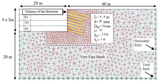
Figure 1.
The scheme of the numerical model in PLAXIS.V8.3.
One of the methods to test whether the model boundaries are located a sufficient distance from the area of interest is to change the fixities (e.g., add and remove vertical fixity at the vertical boundaries) to see if this affects the key outputs. If no significant effect is observed, then the boundaries are located sufficiently far away [20]. A sensitive analysis has been done on the model under different fixities and boundary conditions. The stress state outputs were checked; stress changes were less than 5% at the model boundaries and displacements, and no significant effect on the results was achieved by increasing the dimensions [20]. The results of the sensitivity analysis in the horizontal direction are shown in Figure 2. From Figure 2, there are no significant changes in maximum displacement that can be observed after 60 m in the horizontal direction. Figure 3 shows the variation in the vertical dimension versus safety factor. It can be seen that by increasing the vertical dimension after 28 m, there is no significance in the safety factor of the wall and also no significant changes in displacement and stresses.
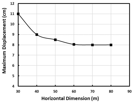
Figure 2.
Sensitive analysis of the horizontal dimension on the maximum displacement of the wall.

Figure 3.
Sensitive analysis of the vertical dimension on the safety factor of the wall.
The period of the soil-wall system is 4H/VS, where H is the thicknesses of soil, and vs. is the shear wave velocity [21,22]. The first period of the wall is 1.68 s.
2.2. Model Verification
The finite element model was validated by comparison with a back-predicted result from a full-scale test carried out in 1986 for the French national research project CLOUTERRE [21]. The CLOUTERRE project’s soil nailed wall is 7 m high and 7.5 m wide. Figure 4 depicts a cross-section of the soil nailed wall.
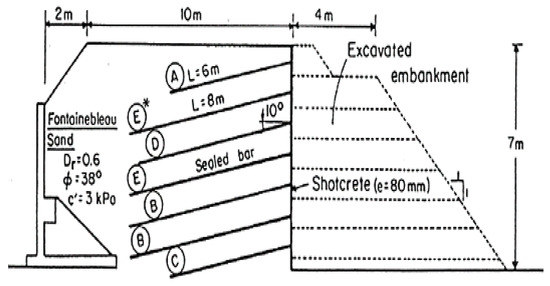
Figure 4.
The CLOUTERRE project’s soil nailed wall geometric profile.
In that test, five different types of nails were used, each labeled A, B, C, D, and E. The lengths of nails for types A, B, C, D, and E are 6 m, 8 m, 6 m, 7.5 m, and 8 m, respectively. Stepped excavation was used to build the wall, with 1 m of excavation alternated with nail installation. The nail lengths ranged from 6 to 8 m and were inclined at a slope of 10 degrees to the horizontal plane. Table 1 represents the detailed parameters of the soil nail wall for backfill soil and the foundation. The 15-node triangular elements are used for this modeling. The Finite element modeling of the CLOUTERRE project is shown in Figure 5. The analysis has been carried out based on the stage of the construction. Figure 6 shows the maximum internal forces in nails compared with Fan and Luo [22] and Plumelle et al. [23]. There is a reasonable comparison between numerical modeling. Figure 7 depicts a comparison of computed maximum tensile forces in nails. The computed and assessed findings are reasonably consistent. The slight differences between the numerical simulation and the test results are related to the following factors:
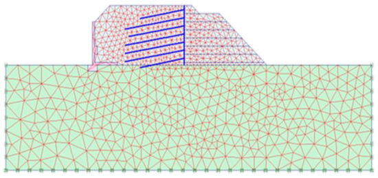
Figure 5.
A scheme of finite element modeling of the CLOUTERRE project.
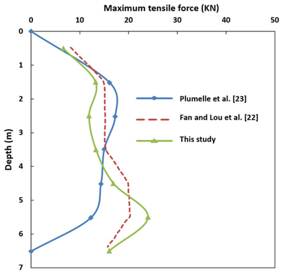
Figure 6.
Maximum tensile forces (Tmax) in the nails.
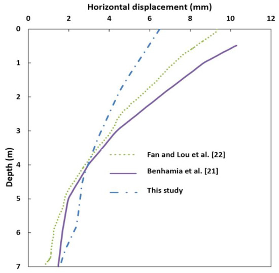
Figure 7.
Maximum lateral displacements in the backfill at 2 m from the wall.
- The number of parameters: The existence of various materials in this research (soil, shotcrete, nail) has led to a large number of parameters being required to model this issue. Nineteen parameters are needed to model this problem, and due to insufficient material test information in different locations of the test, the probability of error in numerical simulation is increased.
- Behavioral model: Due to inherent uncertainties in the field tests, exact modeling of the soil and materials is not possible.
- Error in test data collection: Uncertainties always accompany the installation of sensors and monitor the behavior in the test.
3. Soil Modeling and Material Properties
A soil nail wall with a height of 8 m was used as horizontal levels were taken for backfill soil previously studied by the author [4]. Furthermore, in this study, the material behind the wall was considered to be homogenous. Wall design was produced based on the allowable strains method and using FHWA guidelines. The characteristics of material properties are presented in Table 2 and Table 3 to model the soil-nail system numerically. The three behavioral models, MC, HS, and HSS, were used to model the wall as their results on maximum horizontal displacement and axial forces generated in the nails are compared after each step of excavation. In what follows, a brief description of the behavioral models, MC, HS, and HSS, as well as the major parameters used here, will be offered. The soil condition in this study is a dry soil. The plate element was used to model the nail, shotcrete. The length of nails is 6 and 8 m. The parameters used for this purpose were chosen based on Feng et al. [24] and other similar works, and their values and descriptions are presented in Table 3. It must be noted that was determined.
3.1. Mohr-Coulomb Model (MC)
In order to model the behavior of the linear elastic-perfectly plastic material, the Mohr-Coulomb (MC) model was used along with five major parameters. The model applies a combination of Hooker’s law and Coulomb’s failure criteria [25]. The parameters used in the model are divided into elastic and plastic parameters. The model includes: Young’s Modulus (E), Poisson ratio (V), and the plastic parameters of the model involve soil friction angle (ϕ), cohesion (C), and dilatancy angle (ψ).
3.2. Hardening Soil Model (HS)
The hardening soil model is a robust behavioral model for simulating the behavior of a variety of hard and soft soils. Among the model’s major characteristics, we can refer to shear and compressive hardening and the failure to be stable in the model’s yield level, and the change in it as plastic strains go up. As one major difference between the Hardening Soil (HS) and Mohr-Coulomb (MC) model is the stiffness dependency on the present model’s strain level.
The main idea for formalizing this model is the hyperbolic relationship between axial strain and diversionary strain in relation to triaxial loading. The main parameters of the model include strength parameters φ and Ψ, C as such stiffness parameters and which can control the behavior of the soil deformation as it is presented in Table 2, and the unloading-reloading reference modulus, . The extent to which stiffness is dependent on strain level is determined by the factor m. m value is laid in the range of zero to one. The relationship between the strain and the deviatoric stress is shown in Figure 8.
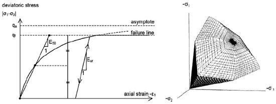
Figure 8.
The stress and strain relation.
3.3. The Hardening Soil Model with Stiffness Effect from Small Strains (HSS)
The HSS model that accounts for the increased stiffness of soils at small strains is developed from the hardening soil model. According to the research, the soil materials revealed higher stiffness in small strains. However, this went unnoticed in most behavioral models such as Mohr-Coulomb and the hardening soil model. Benz [26] considered the effect of the high stiffness of building materials on small strains by making some corrections to the hardening soil. In order to exert the effect of non-linearly raising the stiffness in strains smaller than engineering strains, the parameters and previous parameters were inserted in the HS model, which made a new model called HSS. consists of initial shear modulus, as does shear strain when shear modulus value reaches . The HSS model shows a lesser failure strain than HS.
3.4. Nail Correspondence Parameters
Normally, plain elements are used to model the nailing system in the state of plain strain numerically. In practice, different models are used for calculating nail input parameters. Using equal elasticity modulus is a correct approach to model an embedded nail system. The equal elasticity modulus is calculated by considering the elastic stiffness covering the injection as well as the interior nail rebar and based on material resistance principles:
where stands for the elasticity modulus of the interior nail rebar, stands for the elasticity modulus of injected materials, K stands for interior cross rebar, equals the overall area of the embedded nail system, equals the embedded pure level, and equals to the elastic modulus of the nails. If we present the horizontal distance between nails by Sh, the extent of the axial stiffness of the injected nail system is measured by from Equation (2):
3.5. Overall Procedure of Numerical Modeling
As for the input, the PlAXIS.V8.3 geometry software, which involved the nails and shotcrete procedures, was to be modeled. In what followed, the boundary conditions and the geometry of the construction process were defined, and material parameters were inserted. After completing these processes, appropriate finite element meshes were selected and prepared to be meshed based on this. As shown in Figure 1, the selected mesh size was made finer by as much as one degree to raise the accuracy of the calculations around the nails. With the completion of the generating model, , the procedure was used for generating sustainable strains. It must be noted that the value of was considered much the same as based on Jackie’s equation.
Having completed the construction of the model in input, we arrived at the calculation of the software. In this section, the procedure of the stages for defining and analyzing soil excavation and the implementation based on real stages were chosen, in the sense that the excavation and installation of the nailing system and shotcrete procedure were defined within four calculation phases, , as is shown in Figure 1. At each stage of construction, one 2-m layer of the sustainable soil was made inactivated. The nailing system and shotcrete procedure would be installed by activating structural elements used for modeling. The type of analysis would be adjusted in the plastic calculation mode.
At the end of each stage, we aimed to determine the reliability factor related to Phi/C Reduction analysis, which is based on strength reduction.
The model was run with the standard fixities and earthquake boundaries. Furthermore, the model’s width was selected in such a way that the influence of boundary conditions was minimized in the results. The Rayleigh damping was used to consider material damping [27]:
where C denotes damping, K denotes stiffness, M denotes mass, and α and are the Rayleigh parameters measured:
The critical damping ratio is 0.05, and is the frequency of the system in the first and the second mode [28].
3.6. The Effect of Behavioral Models on Global Stability
The results of the global safety factor are presented at each stage of construction by using the three behavioral models in Figure 9. From Figure 9, every three models show similar results for global safety factors at different stages, and there is no significant difference between the values obtained from HS and HSS behavioral models and those of MC.
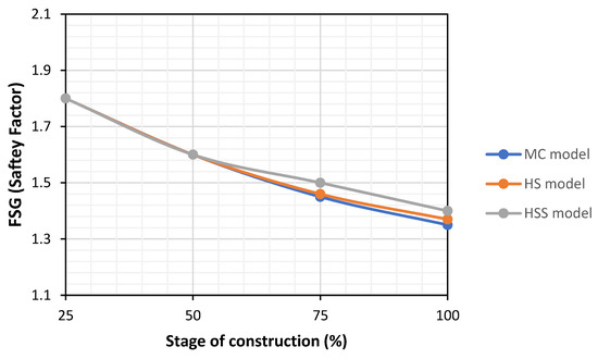
Figure 9.
The global safety factor of the model at the stage of construction.
3.7. The Effect of Modeling Approach on the Maximum Horizontal Displacement of the Soil Nailed Wall System
Figure 10 shows the effects of the modeling approach on the maximum lateral displacement of the wall during the construction stage. From Figure 10, it can be clearly obtained that the MC model estimated a lateral displacement higher than HS and HSS. This is related to the linear behavior of the MC model prior to the yielding state. Therefore, it can be shown that the application of HS and HSS models provides more reasonable results than the MC model. The maximum lateral displacements of the three models were shown at each phase of modeling in Figure 10.
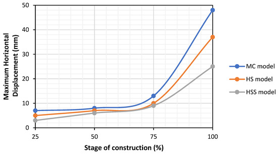
Figure 10.
The maximum horizontal displacement of the wall.
3.8. The Effect of Behavioral Models on Axial Forces Generated in the Nails
Figure 11 and Figure 12 show the maximum axial force generated at the unit of nail length at different stages of excavation and under different depths of installment, respectively. Axial forces in the nail at the HSS model are a bit higher than the HS and MC models.
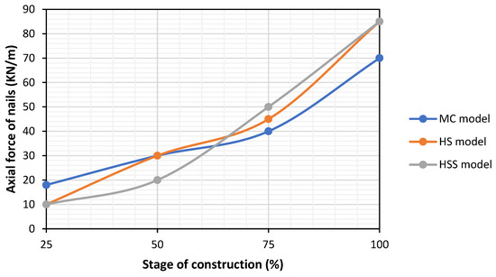
Figure 11.
The maximum axial force of nail with construction stages.
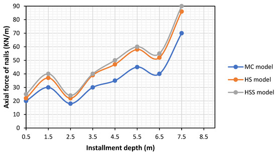
Figure 12.
The maximum axial force of nail with installment depth.
It has been shown that by implementing the modeling nailed walls in soft soils, the use of robust behavioral models such as HS or HSS leads to more reliable results compared with the MC model. It is also observed that the HSS model shows a lower value of displacement at the height of the wall than the HS and MC model, which is due to the consideration of the increased hardness at small strains by the HSS model. The application of behavioral models such as HS and HSS delivers more appropriate results than those of the MC model. In this paper, the HSS model is used for Incremental Dynamic Analysis (IDA) and developing fragility curves.
4. Seismic Ground Motion Records
A relationship is needed between the ground motion records as our input and structural damage as our output to allow for comparison between them. How the models of the wall and also the input ground motions are selected is every important. When a nonlinear time history is performed on a structure, all the nonlinearity of the members is taken into account. The responses of the wall are subsequently dependent on the characteristics of earthquake ground motions. Therefore, the frequency content, intensity and ground type have a great effect on the response of the wall. A reasonable intensity measure and structural damage can lead to a good correlation. Many different intensity measures were suggested to describe the severity of the earthquake ground motion, such as PGA, peak ground velocity (PGV), peak ground displacement (PGD), spectrum intensity (SI), the time duration of strong motion (Td), etc. In this research, PGA and Sa(T1,5%) are used as intensity measures.
PSDA requires an appropriate earthquake record selection. According to FEMA-P58 [29], the earthquake record bin needs to be unbiased to any site-specific seismological characteristic. The other significant point is that the earthquake bin should cover a wide range of structures located in different seismic zones. Therefore, the bin should be structural type independent. FEMA-P695 [30] developed a general far-field record.
Table 3 shows the characteristics of 20 earthquake ground motion records with different ranges of PGA from medium to strong motions, which are used to perform incremental dynamic analysis (IDA). This set of records were selected according to the criteria proposed by FEMA-P695 [30].
Figure 13 shows the acceleration response spectra with a 5% damping ratio of the recorded ground motions. Figure 14 represents the different percentiles of acceleration response spectra with a 5% damping ratio. The range of the PGA is between 0.21 g to 0.82 g. The spectral acceleration figures also contain a wide range of Sa (T1,5%) at the fundamental period of the soil nail walls.
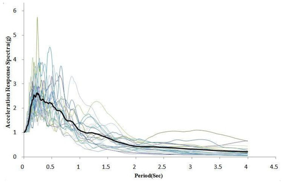
Figure 13.
Response acceleration spectra of earthquake records.
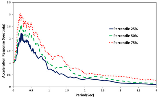
Figure 14.
The percentiles of acceleration spectra of earthquake records.
The records are listed in Table 4, and the criteria are presented as follow:
Table 4.
Characteristics of the earthquake ground motion histories [30].
- (a)
- Magnitude > 6.5
- (b)
- Distance from source to site >10 km (average of Joyner-Boore and Campbell distances) [31]
- (c)
- Peak Ground Acceleration (PGA) > 0.2 g and Peak Ground Velocity (PGV) > 15 cm/s
- (d)
- Soil shear wave velocity, in upper 30 m of soil, greater than 180 m/s
- (e)
- Lowest useable frequency <0.25 Hz, to ensure that the low-frequency content was not removed by the ground motion filtering process
- (f)
- Strike-slip and thrust faults (consistent with California)
- (g)
- No consideration of spectral shape
- (h)
- No consideration of station housing, but PEER-NGA records were selected to be “free-field”
5. Incremental Dynamic Analysis (IDA) and Fragility Curves
5.1. Incremental Dynamic Analysis (IDA)
One of the methods that has been considered by the researchers in the field of performance-based earthquake engineering is incremental dynamic analysis (IDA). This method could prepare valuable information about seismic demand and capacity, estimating the response of structures by increasing the intensity level of ground motion and predicting the probability of reaching or exceeding a specific structural damage level for a given earthquake intensity (PGA and Sa(T1,5%)). To perform IDA, a proper nonlinear structural model is needed as the first step. Then, a suite of records (at least 20) are compiled, scaled to 1.0 g and implemented with an increment increase of 0.1 g until they reach the extensive performance level [31,32,33,34,35,36,37]. For each record, dynamic analysis was carried out and data were post-processed. Total nonlinear analysis is more than 500. We can generate the IDA curves of the wall response with a damage measure and intensity measure. Figure 15 and Figure 16 show the obtained IDA curves from a full nonlinear time history analysis. The Engineering Demand Parameter (EDP) is the maximum drift ratio of the wall, and the intensity measure in Figure 15 is PGA and Sa(T1,5%) in Figure 16. A suitable intensity measure is an efficient IM when the dispersion of the data is less. In this study, the results show that the dispersion of the PGA is higher than Sa(T1,5%), which shows that Sa(T1,5%) is more efficient than PGA for the considered wall. The current research is based on the IDA results in terms of dispersion, as shown in Table 5, based on Equations (6) and (7). In the following section, Bayesian linear regression is implemented to consider the efficiency of the IMs.
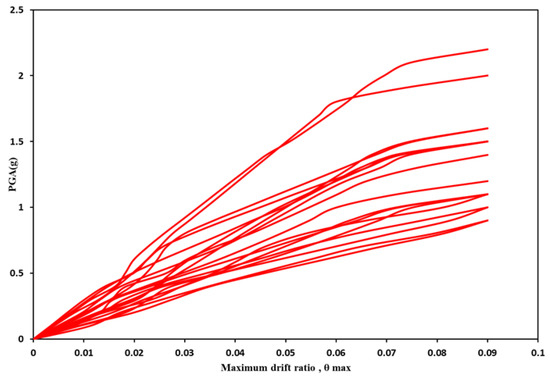
Figure 15.
IDA curves using PGA as an intensity measure.
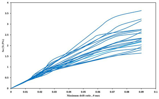
Figure 16.
IDA curves using PGA as an intensity measure Sa(T1,5%).
Table 5.
Damage States (DS) for wall displacements ratio [34].
Intensity Measures (IM) and Damage States (DS)
The IDA results are generally presented as a relation between Engineering Demand Parameter (EDP) and Intensity Measure (IM). The relation between (seismic demand) SD and (intensity measure) IM is estimated as [13]:
The coefficients of a and b using linear regression rewrite Equation (5) as:
The following criteria (efficiency and sufficiency) can classify different intensity measures to select the optimal intensity measure. In this paper, the wall displacements ratio was utilized to define the performance levels in Table 5.
5.2. Fragility Function Methodology
The fragility function was formulated by Cornell et al. [35], and the fragility curves are presented as a lognormal distribution:
= Standard normal cumulative distribution function
= Median value of the structural demand in terms of seismic intensity
= Logarithmic standard deviation, or dispersion, of the demand conditioned on the IM.
6. Bayesian Statistical Inference
Consider as a vector of explanatory functions formulated in terms of independent variables collected in vector . is a response variable predicted by:
where are called model parameters, is a standard normal random variable, and is standard deviation of model error. Traditionally, classical regression is applied to compute the point estimation of model parameters . It is clear that the point estimation, based on information obtained from a finite size sample population, is incomplete and uncertain. Conversely, Bayesian linear regression can express our uncertainty by considering model parameters as random variables and determines the probability distribution of the coefficients using the Bayesian updating rule [25]:
where denotes posterior distribution representing our updated knowledge about the coefficients, represents the likelihood function representing the objective information on gained from a set of observations, denotes the prior distribution reflecting our knowledge about parameters prior to obtaining observations, and is a normalizing factor. In this case, lower bound data and/or upper bound data are not available, such as data collected in this study, and the probabilistic model of interest is formulated as a linear function of , so a closed-form solution can be found for Equation (6) [36,37,38]. Under the normality assumption on and a non-informative prior, Box and Tiao [39] show that the posterior distributions of and , denoting the vector of model parameters , are a multivariate t distribution and an inverse chi-square distribution, respectively.
where is an by dimensional matrix, which contains all observations of explanatory functions. Additionally, is the n-dimensional vector of response variable observations. Once posterior distribution is known, mean vector and the covariance matrix can be computed as follows:
According to the above description and those presented in the previous section, the procedure implemented in the present study to develop the demand model is graphically exhibited in Figure 17.
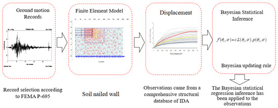
Figure 17.
Bayesian regression demand model procedure.
6.1. Efficiency of an Intensity Measure (IM)
The developed regression-based demand model—the maximum drift demand model of the wall in terms of PGA and Sa(T1,5%) in the form of Equation (7)—is constructed based on the above definition. Table 6 indicates model parameters obtained from IDA and Bayesian regression analysis.
Table 6.
Bayesian regression model parameters in Equation (7).
The posterior correlation coefficients computed between the regression coefficients (model parameters a, b) are also presented in Table 7 and Table 8.
Table 7.
Correlation matrix of regression coefficients implemented in the model in terms of PGA.
Table 8.
Correlation matrix of the regression coefficients implemented in the model in terms of Sa(T1,5%).
In addition, Figure 18 and Figure 19 show the diagnosis of regression demand graphically. The model projections were plotted against obtained data. The Q-Q graph shows the normality of the model. Similarly, the accuracy of a model is determined by the degree to which plotted prediction data correspond with a 45° line. Furthermore, if the residuals appear roughly horizontal on both sides of the zero axes, the suggested regression model is appropriate in terms of heteroscedasticity. Technical texts provide more detail on regression diagnosis strategies. Based on Table 6, Table 7 and Table 8, the Sa(T1,5%) is more efficient for retaining walls to be considered as an Intensity Measure (IM).
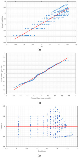
Figure 18.
Graphical diagnoses of the regression model PGA; (a) model prediction; (b) Quantile-Quantile graph; (c) residual graph.
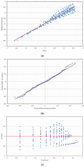
Figure 19.
Graphical diagnoses of the regression model, Sa(T1,5%); (a) model prediction; (b) Quantile-Quantile graph; (c) residual graph.
6.2. Sufficiency of an Intensity Measure (IM)
Sufficiency is a criterion that shows the IM is statistically independent of earthquake ground motions such as Magnitude (M) and Epicentral distance (R). Regression analysis is needed on the residuals. Lower p-values show that the regression estimate’s coefficient is statistically important. A p-value of 0.10 was the cutoff for an insufficient IM [13]. The p-values are 0.52 and 0.61 based on R and M, which shows that the Sa(T1,5%) is a sufficient IM for conditioning the probabilistic seismic demand analysis (PSDA) (see Figure 20 and Figure 21).
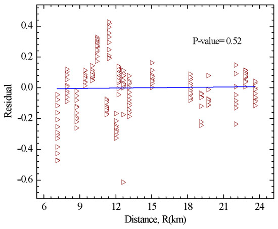
Figure 20.
p-value analysis to implement the conditional statistical independence from epicenteral distance (R).
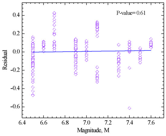
Figure 21.
p-value analysis to implement the conditional statistical independence from magnitude (M).
7. Fragility Analysis Results
Fragility curves of the soil wall for three different performance levels are presented in Figure 22 and Figure 23 for the Slight, Moderate, and Extensive damage states for Sa(T1,5%) and PGA. The analytical fragility curves show the failure probability of the wall for a certain values’ intensity measures. It is strongly suggested to consider other important intensity measures to find a suitable IM that has less dispersion in data. The reliable fragility curves are based on Sa(T1,5%), which provides a more accurate failure probability since the IM is more efficient and sufficient.
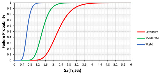
Figure 22.
The soil nail wall’s fragility curves with respect to Sa (T1,5%).
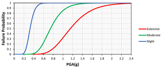
Figure 23.
Fragility curves of the soil nail wall with respect to PGA.
8. Conclusions
In this paper, detailed finite element modeling of the soil nailed wall was completely studied. Three different approaches for soil modeling were considered (MC, HS, and HSS). Detailed and verified numerical modeling was presented. We have tried to achieve analytical seismic fragility curves of the typical soil nailed wall. Two standard intensity measures were considered (PGA and Sa(T1,5%)). A total of 20 suit records were selected, and incremental dynamic analysis was applied to the wall. Bayesian linear regression was used to develop the demand model and selection of the proposed intensity measure. The results show that the selection of the records has a great effect on the response of the structures and the further findings of the study. Comparison of IDA results and the efficiency and sufficiency of the IMs shows that Sa(T1,5%) is more suitable for these types of walls with respect to PGA because of its efficiency and sufficiency.
Author Contributions
Conceptualization, M.B. and A.H.K.; methodology, M.B. and A.H.K.; validation, M.B., A.H.K. and M.J.; formal analysis, M.B.; writing—original draft preparation, M.B.; writing—review and editing, M.B., A.H.K. and M.J.; All authors have read and agreed to the published version of the manuscript.
Funding
This research received no external funding.
Institutional Review Board Statement
Not applicable.
Informed Consent Statement
Not applicable.
Data Availability Statement
Data will be made available upon request.
Conflicts of Interest
The author declares no conflict of interest.
References
- Basoz, N.; Kiremidjian, A.S. Evaluation of Bridge Damage Data from the Loma Prieta and Northridge, California Earthquakes; Multidisciplinary Center for Earthquake Engineering Research: Buffalo, NY, USA, 1998. [Google Scholar]
- Shinozuka, M.; Banerjee, S.; Kim, S.H. Fragility Considerations in Highway Bridge Design (No. MCEER-07-0023); Multidisciplinary Center for Earthquake Engineering Research: Buffalo, NY, USA, 2007. [Google Scholar]
- Shinozuka, M.; Feng, M.Q.; Lee, J.; Naganuma, T. Statistical analysis of fragility curves. J. Eng. Mech. 2000, 126, 1224–1231. [Google Scholar] [CrossRef]
- Ardakani, A.; Bayat, M.; Javanmard, M. Numerical modeling of soil nail walls considering Mohr Coulomb, hardening soil and hardening soil with small-strain stiffness effect models. Geomech. Eng. 2014, 6, 391–401. [Google Scholar] [CrossRef]
- Chu, L.M.; Yin, J.H. A Laboratory Device to Test the Pull out Behavior of Soil Nails. Geotech. Test. J. 2015, 28, 499–513. [Google Scholar] [CrossRef]
- Chu, L.M.; Yin, J.H. Comparison of Interface Shear Strength of Soil Nails Measured by Both Direct Shear Box Tests and Pull-Out Tests. J. Geotech. Geoenvironmental Eng. 2005, 131, 1097–1107. [Google Scholar] [CrossRef]
- Bayat, M.; Daneshjoo, F.; Nisticò, N. The effect of different intensity measures and earthquake directions on the seismic assessment of skewed highway bridges. Earthq. Eng. Eng. Vib. 2017, 16, 165–179. [Google Scholar] [CrossRef]
- Shome, N.; Cornell, C.A.; Bassurro, P.; Carballo, J.E. Earthquakes, records, and nonlinear responses. Earthq. Spectra 1998, 14, 469–500. [Google Scholar] [CrossRef]
- ATC. Earthquake Damage Evaluation Data for California; ATC-13; Applied Technology Council: Redwood City, CA, USA, 1985. [Google Scholar]
- FEMA. Earthquake Model. HAZUS-MH MR1: Technical Manual; Federal Emergency Management Agency: Washington, DC, USA, 2003.
- Shome, N. Probabilistic Seismic Demand Analysis of Non-linear Structures. Ph.D. Thesis, Stanford University, Stanford, CA, USA, 1999. [Google Scholar]
- Tothong, P.; Luco, N. Probabilistic seismic demand analysis using advanced ground motion intensity measures. Earthq. Eng. Struct. Dyn. 2007, 36, 1837. [Google Scholar] [CrossRef]
- Padgett, J.E.; Nielson, B.G.; DesRoches, R. Selection of optimal intensity measures in probabilistic seismic demand models of highway bridge portfolios. Earthq. Eng. Struct. Dyn. 2008, 37, 711–726. [Google Scholar] [CrossRef]
- Bayat, M.; Daneshjoo, F.; Nisticò, N. A novel proficient and sufficient intensity measure for probabilistic analysis of skewed highway bridges. Struct. Eng. Mech. 2015, 55, 1177–1202. [Google Scholar] [CrossRef]
- Baker, J.W.; Allin Cornell, C. A vector-valued ground motion intensity measure consisting of spectral acceleration and epsilon. Earthq. Eng. Struct. Dyn. 2005, 34, 1193–1217. [Google Scholar] [CrossRef]
- Luco, N.; Cornell, A.C. Structure-specific scalar intensity measures for near-source and ordinary earthquake ground motions. Earthq. Spectra 2007, 23, 357–392. [Google Scholar] [CrossRef]
- Tiznado, J.C.; Rodríguez-Roa, F. Seismic lateral movement prediction for gravity retaining walls on granular soils. Soil Dyn. Earthq. Eng. 2011, 31, 391–400. [Google Scholar] [CrossRef]
- Choobbasti, A.J.; Kutanaei, S.S.; Ahangari, H.T.; Kardarkolai, M.M.; Motaghedi, H. Comparison of different local site effect estimation methods in site with high thickness of alluvial layer deposits: A case study of Babol city. Arab. J. Geosci. 2020, 13, 1–9. [Google Scholar] [CrossRef]
- Tavakoli, H.; Kutanaei, S.S.; Hosseini, S.H. Assessment of seismic amplification factor of excavation with support system. Earthq. Eng. Eng. Vib. 2019, 18, 555–566. [Google Scholar] [CrossRef]
- Rawlings, C. Geotechnical finite element analysis-a practical guide. In Proceedings of the Institution of Civil Engineers-Civil Engineering; ICE Publishing: London, UK, 2017; Volume 170, pp. 152–153. [Google Scholar]
- Unterreiner, P.; Benhamida, B.; Schlosser, F. Finite element modelling of the construction of a full-scale experimental soil-nailed wall. French National Research Project CLOUTERRE. In Proceedings of the Institution of Civil Engineers-Ground Improvement; ICE Publishing: London, UK, 1997; Volume 1, pp. 1–8. [Google Scholar]
- Fan, C.C.; Luo, J.H. Numerical study on the optimum layout of soil–nailed slopes. Comput. Geotech. 2008, 35, 585–599. [Google Scholar] [CrossRef]
- Plumelle, C.; Schlosser, F.; Delage, P.; Knochenmus, G. French National Research Project on Soil Nailing: Clouterre; Geotechnical Special Publication No.25; ASCE: New York, NY, USA, 1990; pp. 660–675. [Google Scholar]
- Feng, X.; Xia, X.-H.; Wang, J.-H. The Application of small strain model in excavation, The National Natural Science Foundation of China (No.50679041). J. Shanghai Jiaotong Univ. 2009. [Google Scholar] [CrossRef]
- Plaxis, B. PLAXIS 3D Foundation Material Models Manual; PLAXIS: Rhoon, The Netherlands, 2008. [Google Scholar]
- Benz, T. Small-Strain Stiffness of Soils and Its Numerical Consequences; University of Stuttgart: Stuttgart, Germany, 2007; Volume 5. [Google Scholar]
- Ibrahim, K.M.H.I.; Ibrahim, T.E. Effect of historical earthquakes on pre-stressed anchor tie back diaphragm wall and on near-by building. HBRC J. 2013, 9, 60–67. [Google Scholar] [CrossRef]
- Noorzad, R.; Omidvar, M. Seismic displacement analysis of embankment dams with reinforced cohesive shell. Soil Dyn. Earthq. Eng. 2010, 30, 1149–1157. [Google Scholar] [CrossRef]
- Agency, F.E.M. Quantification of Building Seismic Performance Factors; FEMA P695: Washington, DC, USA, 2001. [Google Scholar]
- Agency, F.E.M. Seismic Performance Assessment of Buildings; FEMA P58: Washington, DC, USA, 2018. [Google Scholar]
- Boore, D.M.; Joyner, W.B.; Fumal, T.E. Estimation of Response Spectra and Peak Accelerations from Western North American Earthquakes: An Interim Report; Open-File Report 93-509; U.S. Geological Survey: Menlo Park, CA, USA, 1993.
- Vamvatsikos, D.; Jalayer, F.; Cornell, C.A. Application of incremental dynamic analysis to an RC-structure. In Proceedings of the FIB Symposium on Concrete Structures in Seismic Regions, Athens, Greece, 6–8 May 2003; pp. 75–86. [Google Scholar]
- Alam, M.S.; Bhuiyan, M.R.; Billah, A.M. Seismic fragility assessment of SMA-bar restrained multi-span continuous highway bridge isolated by different laminated rubber bearings in medium to strong seismic risk zones. Bull. Earthq. Eng. 2012, 10, 1885–1909. [Google Scholar] [CrossRef]
- Zamiran, S.; Osouli, A. Seismic motion response and fragility analyses of cantilever retaining walls with cohesive backfill. Soils Found. 2018, 58, 412–426. [Google Scholar] [CrossRef]
- Cornell, A.C.; Jalayer, F.; Hamburger, R.O. Probabilistic basis for 2000 SAC federal emergency management agency steel moment frame guidelines. J. Struct. Eng. 2002, 128, 526–532. [Google Scholar] [CrossRef]
- Gardoni, P.; Der Kiureghian, A.; Mosalam, K.M. Probabilistic capacity models an and d fragility estimates for reinforced concrete columns based on experimental observations. J. Eng. Mech. 2002, 128, 1024–1038. [Google Scholar] [CrossRef]
- Kia, M.; Amini, A.; Bayat, M.; Ziehl, P. Probabilistic Seismic Demand Analysis of Structures Using Reliability Approaches. J. Earthq. Tsunami 2020, 2150011. [Google Scholar] [CrossRef]
- Kia, M.; Banazadeh, M.; Bayat, M. Rapid seismic loss assessment using new probabilistic demand and consequence models. Bull. Earthq. Eng. 2019, 17, 3545–3572. [Google Scholar] [CrossRef]
- Box, G.E.; Tiao, G.C. Bayesian Inference in Statistical Analysis; John Wiley & Sons: Hoboken, NJ, USA, 2010; Volume 40. [Google Scholar]
Publisher’s Note: MDPI stays neutral with regard to jurisdictional claims in published maps and institutional affiliations. |
© 2021 by the authors. Licensee MDPI, Basel, Switzerland. This article is an open access article distributed under the terms and conditions of the Creative Commons Attribution (CC BY) license (https://creativecommons.org/licenses/by/4.0/).