Abstract
The relationship between economic growth and environmental impact has become a recurrent subject of research in recent years. Currently, results that indicate that the accumulation of economic growth leads to a reduction in environmental impact coexist with others that do not show any evidence in this respect. This paper aims to analyse this relationship using Material Flow Analysis through the two most frequent methods: territorial or production and consumption. For this purpose, data from China, the United Kingdom and the USA from 1990–2017 are used. The results show that the method used influences the conclusions, mainly due to differences in the accounting of physical trade flows. The production method, in which physical trade flows coincide with monetary trade flows, tends to underestimate the material consumption of rich, importing countries, while overestimating that of exporting countries. Policies based on this method have limited capacity to reduce global environmental impacts. The consumption method allows the environmental impact to be allocated to each country in a way that is more in line with its true material requirements.
1. Introduction
Since the Industrial Revolution, the impact of economic activity on nature has continued to grow, and it was not until the second half of the 20th century that the problem began to receive attention [1,2,3]. The realisation of phenomena associated with climate change and the first situations of scarcity of certain resources were decisive situations for the preservation of the environment to begin to appear as an objective of many governments and institutions [4,5,6,7]. At the end of the 1980s, the concept of sustainable development was defined, proposing environmentally friendly economic growth without compromising the needs of future generations [3]. At the same time, different studies were developed that related economic growth with the reduction of environmental impact, such as that of Shafik and Bandyopadhyay [4] or that of Panayotou [5], who used for the first time the so-called Environmental Kuznets Curve (EKC) in his analyses.
The EKC hypotheses indicate that environmental impact maintains an inverse relationship with GDP in countries with subsistence economies, evolving jointly as development increases, until a turning point is reached, from which the relationship is reversed [5]. Thus, thanks to specialisation in technology-intensive industries and the service sector, brought about by the rise of Information and Communication Technologies (ICTs), economies with high levels of development would be able to reduce their dependence on the environment [5,6]. The EKC hypothesis has made the relationship between GDP and environmental impact the subject of many studies. There are many studies that verify the EKC hypotheses, mostly focused on a territorial or local production approach and on rich countries or countries with particular characteristics (small size or high sectoral specialisation, for example) [7,8,9]. Paradoxically, the decoupling of GDP and environmental impacts is more significant in periods of recession or low economic growth [10]. Moreover, there is more evidence of decoupling when analysing waste and emissions [11,12] than when analysing material consumption [13].
On the other hand, the field of ecological economics is more sceptical about the ability of policies based on sustainable development to reduce environmental impacts [10,14,15,16]. From this perspective, a common problem in studies is the effect of high GDP in rich countries on efficiency indicators, which leads to an overestimation of the sustainability of rich countries, even though their environmental impact is higher than that of less developed countries [17,18,19]. Thus, efficiency gains do not necessarily imply a lower environmental impact in absolute terms [18,20,21]. On the other hand, studies conducted on a global scale show that the global environmental impact has continued to grow [19,22], while analyses based on the final consumption perspective attribute a greater environmental impact to rich countries than those using a territorial approach [18,19,23,24]. In this sense, work based on local production has limitations when it comes to considering the effects of international trade and the relocation of production on the distribution of environmental impact [23,24,25,26].
There are multiple ways to measure the impact of economic activity on the environment, but most can be classified as input (resources extracted from nature) or output (waste discharged into nature) methods [27]. The research presented in this article focuses on the analysis from an input perspective, studying material flows using the tools of Material Flow Analysis (MFA). Although material flows do not provide specific information about the impact of socio-economic activity on nature, they are appropriate to approximate the pressure exerted by socio-economic activity on the environment [23]. Material Flow Analysis (MFA) is a method developed by Ayres and Kneese [28] in the framework of the study of economic externalities, which has subsequently been repeatedly updated [29,30,31,32,33,34], in a process that is still ongoing today. Based on the concept of socio-economic metabolism, which draws an analogy with human societies and living organisms to analyse the relationships between them and nature, the MFA makes it possible to obtain the physical accounting associated with the socio-economic activity of a territory [35,36,37]. Material flows are a key element in the field of socio-economic metabolism, as they act as a physical link between societies and nature [27]. Like any living organism, a society can live using only renewable resources, so it will generate waste that nature’s own mechanisms can transform into reusable resources. However, the exploitation of non-renewable resources has become widespread, causing a double problem: on the one hand, the rate of replenishment of these resources is considerably lower than the rate of exploitation; on the other hand, the waste they generate is not easily assimilated by nature and can cause significant damage to it [20]. Moreover, according to the laws of thermodynamics, the problem of replenishment is much more serious, because each time a resource is used, the energy it contains is irreversibly degraded [38].
The aim of this paper is to analyse whether economic growth becomes independent of environmental impact, measured through material flows, as the level of development increases and the economic structure of a country changes. The study will be carried out with data from three countries, China, United Kingdom and the USA, for the period between 1990 and 2017, using the MFA through the production and consumption methods. The added value of this research lies in the comparison of the two most frequent MFA methods in a heterogeneous group of countries, which are at different points in the evolution of the relationship between economic growth and environmental impact, following the EKC hypotheses. This will make it possible not only to study the relationship between economic growth and material consumption, but also the influence of each approach on the analysis.
2. Materials and Methods
2.1. Material Flow Analysis
There are different methods for assigning the corresponding environmental impact to each territory. Depending on the method used, the material flows of each territory may vary. In this work, the MFA is carried out using the two most common methods, the territorial or production method and the consumption method, which will make it possible to study the differences between the results of the two approaches.
The production approach is the one most widely used by most institutions, as well as the one on which most climate policies are based. This method assigns to each territory the materials consumed in domestic production processes, discounting the final weight of exported goods, and adding that of imported goods [18,23,34,39,40]. In this way, the material flows collected in the trade section correspond to monetary flows [41]. The main indicators of the MFA are:
- Domestic Extraction (DE): is the sum of all materials, biotic and abiotic, extracted from nature and used in economic activity [18,23,34,41,42]. It is common to both approaches;
- Domestic Material Consumption (DMC): results from adding physical imports to EI and deducting exports. Additionally, known as apparent consumption, it includes the materials used in domestic production, including imported products, and excluding exports [20,21,22,23,24];
- Physical Trade Balance (PTB): it is the difference between material imports and exports [18,19,23,34,42,43]. It is constructed inversely to the monetary trade balance because physical flows move in the opposite direction to monetary flows, so its interpretation is also inverse to the usual one [23,42,44].
Using the MFA indicators, other indicators can be composed to analyse the relationship between material flows and economic growth. The most used are efficiency indicators, such as material productivity (GDP/DMC) or material intensity (DMC/GDP) [23]. However, these indicators do not show whether efficiency is improved by a reduction in material consumption. Therefore, they can lead to the interpretation that the sustainability of an economy improves, even if it increases resource consumption, if GDP grows more [17].
Another common way of analysing the evolution of an economy’s material requirements is by looking at the degree of decoupling between GDP and the DMC. Decoupling occurs when the amount of material resources used per unit of GDP decreases [45,46,47]. This can occur when the DMC increases, but to a lesser extent than GDP, which is known as relative or weak decoupling, or when the DMC decreases, which is known as absolute or strong decoupling [19,23,45,48]. It is important to make this distinction because, although in both cases there is an improvement in efficiency, only in the case of absolute decoupling is material consumption reduced [23]. Although dematerialisation is often used as a synonym for decoupling, this only makes sense in the case of absolute decoupling, otherwise material consumption has increased [49].
The degree of decoupling can be analysed by comparing the cumulative growth rates of GDP and DMC over a time interval. For comparisons between territories, it is more practical to use a single indicator such as the decoupling ratio [48], which is constructed as follows:
Decoupling ratio = (DMC/GDP)end of period/(DMC/GDP)beginning of period
Values below one indicates that there is decoupling in the period under consideration, although they do not indicate whether the decoupling is relative or absolute [47]. It is important to note that the indicators obtained using the production method only reflect the final weight of traded goods. Therefore, materials used in production but not incorporated in the final good are not captured in physical trade flows [25,28,29,30].
In contrast, the consumption method imputes to each territory the materials used in the production of the goods consumed by its domestic demand [24]. Thus, physical trade flows include all the materials that are part of the production process of each good, whether they are part of the final good or not [18,41,42]. The physical trade flows that are not captured by the production method are known as indirect flows, because they are not deducted directly, but need to be estimated by looking for the equivalent raw materials in terms of domestic extraction in each territory [18,19,34,41,42]. The indicator for material consumption obtained through the consumption method is known as the Material Footprint and is constructed like the DMC, but accounting for indirect flows in the PTB [19,34,50]. The Material Footprint allows to check the materials that each country needs to mobilise to satisfy its final demand, providing more information about the effects of international trade on material flows [18,19,23,34,51].
2.2. Data
This paper analyses the period from 1990 to 2017, using data from the Global Material Flows Database [52] for the United Kingdom, the USA and China. To facilitate comparability, per capita data will be used where possible and GDP in constant 2010 USD. The period selected is a matter of data availability, as indicators from the consumption perspective are only available since 1990. On the other hand, this period includes relevant economic events such as China’s accession to the World Trade Organization (WTO) or the 2008 crisis.
The countries chosen are of great importance in economic history and have a global influence in many social and cultural aspects. The United Kingdom was the scene of the Industrial Revolution and the first industrial economic power in history, although today it is a service-sector economy. The USA is the country that took over from the United Kingdom at the industrial forefront and the birthplace of mass production and consumption. As in the UK, industry has declined in importance in favour of service-sector activities, but it still retains great importance on a global scale, especially in areas such as R&D. In contrast, China has been a country with little industrial presence until less than half a century ago. With a different economic organisation to that of the main developed countries, its growth from 1980 to the present day has been enormous, driven by an industry that has condensed multiple stages in barely 40 years to compete in the most cutting-edge technologies today.
The countries selected allow for the analysis of three very heterogeneous economies that reflect different characteristics typical of many other economies, facilitating the adaptation of the methodology used to other territories. The United Kingdom is a small country with a high population density and a small resource endowment, which means that it depends on production in other countries [53]. This makes it easier to maintain a contained environmental impact [53,54]. The USA is a very large country with a marked duality in population distribution and a large but declining productive capacity. It also has a remarkable endowment of natural resources, despite which it is a major importer of multiple materials, such as oil [55]. It is one of the countries with the greatest environmental impact [56]. China is also a very large country with a duality like that of the USA in its population distribution [57]. Its productive capacity is enormous, as is its endowment of natural resources, although it needs to import certain materials in large quantities [58]. Together with the USA, it is one of the leading countries in terms of environmental impact [56].
In the years leading up to the 1990s there are some important changes for the context of this paper. In the 1970s, the evolution of oil prices provoked a crisis in most developed countries that particularly affected industry. The subsequent liberalisation of financial activity and the evolution of ICTs favoured the delocalisation of productive activities, increasingly detaching the physical location of the activity from the place where it generates value [59]. The fragmentation of production on a global scale means that many multinationals only maintain their management and service activities in their countries of origin, giving rise to a new form of organisation of production known as Global Value Chains (GVC) [60]. The high profitability of the financial sector affected the productive structure of Western countries, reducing the importance of the industrial sector and subordinating it to financial logic, a process known as the financialisaton of the economy [61,62,63].
In China, the late 1970s saw the beginning of a process of reform of the economic system characterised by gradualism and the importance of the external sector [64,65,66]. Foreign investment has been one of the key factors in the Chinese development process, being the source of the technological transfers that have allowed local industry to evolve [64,65]. Initially, foreign investment was allowed in a limited way and in specific areas, shaping an industrial sector oriented towards manufacturing exports and concentrated in coastal areas, which fostered an important phenomenon of urbanisation of the population [57,67]. Accession to the WTO in the early 2000s is another key to China’s development, as it led to a qualitative and quantitative leap in its export sector [65]. At the same time, it facilitated investments in sectors with a higher technological content, for which China is attractive thanks to its low wage costs and the potential of its large domestic market [68]. In recent five-year plans, new priorities have emerged, such as a focus on domestic demand over the external sector and on an industry capable of competing on quality rather than quantity. More recently, Chinese government planning has begun to incorporate the goal of reducing environmental impact through investment in renewable energy sources and the development of the service sector [69,70].
3. Results and Discussion
3.1. Production Method
Domestic extraction is independent of the approach used in the MFA, as it does not depend on international trade. From an output perspective, trade does not usually have a very large effect on the DMC, so there are no major differences with respect to DE. Figure 1 shows how both series evolve in a very similar way in all countries.
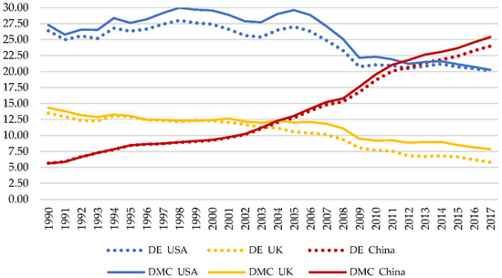
Figure 1.
EI and DMC per capita, tonnes. Source: own elaboration based on data from Global Material Flows Database [52].
Two different trends can be distinguished. On the one hand, the USA and the United Kingdom maintain a declining trajectory for most of the series, with a turning point in 2008, coinciding with the 2008 Crisis. It is noteworthy that the USA values are much higher and are notably more influenced by the 2008 Crisis. Nevertheless, in recent years oil extraction has increased, thanks to techniques such as fracking, promoted by the government as part of its goal of achieving energy independence [55,71]. In the United Kingdom, the downward trend is due to the decline of the coal industry and sector. During the 1980s, most mines were closed, and coal was progressively replaced by other imported energy sources, such as gas [72]. Moreover, part of the difference in extraction and consumption values between the USA and the United Kingdom can be explained by territorial distribution: while the USA has a large surface area and a large endowment of resources, the United Kingdom has a much smaller territory and is poorer in material resources. Consequently, the population density of the United Kingdom is much higher, facilitating a lower consumption of resources in transport, while at the same time it needs to outsource many production processes due to spatial issues, which reduces its DMC [53,54].
On the other hand, China’s trend is increasing and, although starting from very low levels, it has overtaken the USA in recent years. China’s extraction and consumption are driven by the rapid growth of its economy, which demands large quantities of practically all groups of materials. Of note is the extraction and consumption of non-metallic minerals, which include the materials needed to produce cement, as China is by far the largest consumer of this material in recent years [73], due to the major infrastructure and city construction process still underway in the country. The PTB corresponds to the difference between the EI and the DMC and provides information about the effects of international trade on consumption. Figure 2 shows that all three countries show physical surpluses throughout the series, implying that they are net importers of materials.
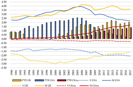
Figure 2.
PTB, tonnes per capita. X: exports, M: imports. Source: own elaboration based on data from Global Material Flows Database [52].
The United Kingdom’s scarce resource endowment and the decline of its industry mean that it needs to import all kinds of products. In the USA, trade flows are mainly determined by fossil fuels and metal ores. After the 2008 crisis, consumption of metal ores fell significantly and dragged down imports, while the focus on domestic fuel extraction reduced external dependence, even allowing exports to increase. China’s surplus grows as it reaches higher levels of development, through imports of resources such as oil and certain food products. More recently, the development of the steel and aluminium industries has made China a major importer of metal ores.
In terms of efficiency, the United Kingdom performs the best, well above the USA, as can be seen in Figure 3. China is still far behind these countries, weighed down by heavy investment in infrastructure. It is important to note that, as discussed above, efficiency indicators that directly compare GDP and DMC tend to favour more developed countries, as their high GDP level smooths the DMC [9].
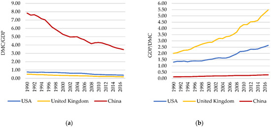
Figure 3.
(a) Material intensity, Kg/USD. (b) Material productivity, USD/kg. Source: own elaboration based on data from Global Material Flows Database [52].
To obtain information on the evolution of a country’s material requirements, it is more appropriate to analyse the degree of decoupling through the growth rates of GDP and the DMC. Table 1 shows the values of the decoupling ratio for the three countries in the time interval studied.

Table 1.
Decoupling ratio (1990–2017). Source: own elaboration based on data from Global Material Flows Database [52].
The decoupling ratio indicates that decoupling occurs in all three cases. As would be expected from its DMC, the United Kingdom has the highest degree of decoupling. More striking is the case of China, which performs better than the USA despite the high growth rate of its DMC. As in the case of the efficiency indicators, the relative nature of this indicator means that a high growth rate of the DMC can be diluted by an even higher GDP growth rate and show as sustainable territories that consume increasing and very high quantities of materials.
The best way to assess a country’s sustainability is to analyse whether dematerialisation occurs. Figure 4 shows the graphical representation of GDP and DMC growth rates for each country, which allows us to analyse both decoupling and dematerialisation. It can be seen how, once again, the 2008 crisis represents a turning point: in the USA, it is the point from which dematerialisation occurs, while in the United Kingdom, which is at dematerialisation values throughout the series, the decline in the DMC intensifies. It is common for periods of low growth or recession to favour dematerialisation in the most developed countries [10]. On the other hand, the 2008 crisis meant an increase in the growth rate of China’s DMC, although this was compensated for by the high value of its GDP growth.
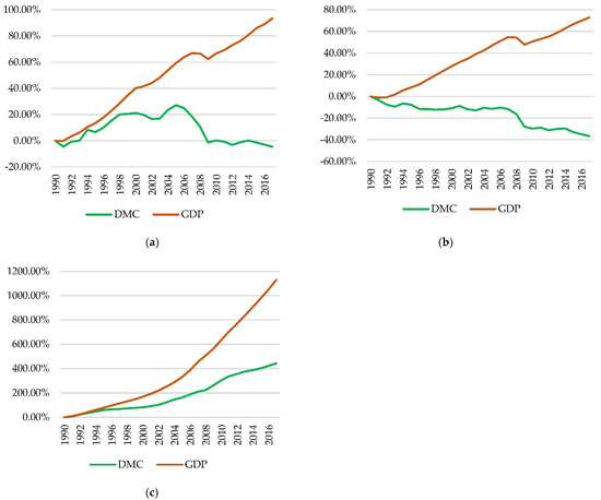
Figure 4.
(a) USA decoupling. (b) UK decoupling. (c) China decoupling. Source: own elaboration based on data from Global Material Flows Database [52].
From the perspective of production, the MFA in these three countries allows us to affirm that it is possible to make economic growth compatible with the reduction of material consumption. While dematerialisation does not occur in the USA until after the 2008 crisis, the United Kingdom maintains a decreasing DMC throughout the series. This situation could fit within the EKC hypothesis [5,7,8], so that the United Kingdom would have passed the turning point of its DMC before the period analysed, while for the USA it would correspond to the 2008 Crisis. In China, although there is decoupling, the DMC grows at a high rate, which could be interpreted as the development phase in which both variables are positively correlated. Table 2 shows a summary of the results of the production method through which these conclusions have been obtained.
Table 2.
Summary of production method data, units per capita. Source: own elaboration based on data from Global Material Flows Database [52].
3.2. Dematerialisation or Relocation?
Decoupling can be understood as a normal consequence of economic operation, since any economic process seeks to maximise output given a limited number of resources. However, dematerialisation implies a reduction in the use of resources, which is not a common occurrence no matter how much efficiency is improved. Efficiency improvements are usually aimed at increasing output, rather than maintaining the same level using fewer resources. In fact, an increase in efficiency in the use of a given resource reduces the cost of the technologies associated with it, leading to a greater use of that resource and, therefore, to an increase in the use of that resource, known as the rebound effect [18,20,21].
In countries where dematerialisation is observed, from the perspective of production, different factors come together, for example: reduced population growth, increased efficiency in the use of resources, a high stock of infrastructures, high population density or specialisation in service activities, known as tertiarization [46,53]. However, the most important factor behind dematerialisation is often the relocation of productive activities to other territories [23,25]. The offshoring processes that richer countries have carried out over the last few decades have caused production chains to be structured on a global scale, taking production centres and, therefore, material consumption away from rich countries [60].
Figure 5 and Figure 6 show how the global distribution of material consumption varies according to the perspective used. The most obvious variations occur in Western countries, mainly in North America and Europe, which have a much higher Material Footprint than their DMC. This can be seen with a shift towards shades closer to yellow and red. In contrast, in regions such as South America or much of Asia, where countries with high levels of material exports are found, there is a shift towards more greenish colours, because they generally have a lower Material Footprint than their DMC. Table A1 in Appendix A contains data that complement the information in this section and reinforce the conclusions drawn. Table A1 in Appendix A contains data that complement the information in this section and reinforce the conclusions drawn. It contains data for 165 countries for 2015, including GDP per capita, Domestic Extraction, Physical Trade Balance, Raw Trade Balance, Mate-rial Footprint, Domestic Material Consumption, and the difference between the latter two, providing a complete overview of each country’s situation.
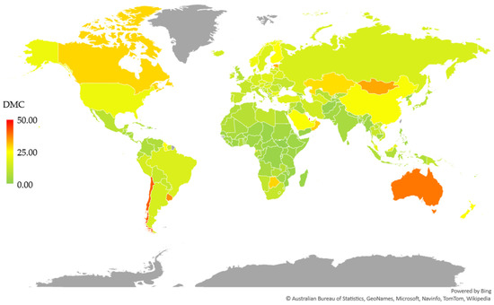
Figure 5.
Domestic Material Consumption tonnes per capita, year 2015. Source: own elaboration based on data from Global Material Flows Database [52] using the Microsoft Excel map creation tool.
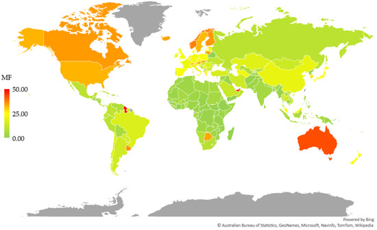
Figure 6.
Material Footprint, tonnes per capita, year 2015. Source: own elaboration based on data from Global Material Flows Database [52] using the Microsoft Excel map creation tool.
Therefore, the production approach underestimates the material consumption of countries with less industrial weight, generally the richest, while overestimating the material consumption of exporting countries [19,74,75]. Through this approach, offshoring reduces material consumption, as production is shifted to other countries. However, the goods produced by the offshored industries are still consumed, so material consumption is maintained. Using the consumption method, it is possible to obtain a more realistic picture of the material requirements of each country [76].
3.3. Consumption Method
As indicated in the methodological section, the consumption perspective focuses on the materials that each country needs to mobilise to satisfy its domestic consumption. This is achieved by attributing to each country the indirect flows associated with its trade flows, so that each country is assigned the consumption of materials associated with the production of its final consumption, regardless of where this production takes place.
Figure 7 shows that import indirect flows are very high in both the United Kingdom and the USA, indicating a high dependence on goods produced elsewhere. Indirect flows linked to exports are much lower and are on a downward trend that may be associated with the decline in local production. The situation is the reverse in China, whose indirect flows are particularly high in exports, due to the role of importer of raw materials and exporter of products that it has acquired in many sectors, such as metals [77]. The indirect flows of its imports, although more moderate, maintain a growing trend, derived from its growing need to import foodstuffs [78], among other things.
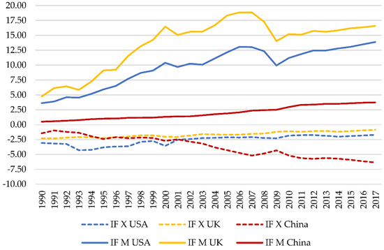
Figure 7.
Indirect trade flows, tonnes per capita. X: exports, M: imports. Source: own elaboration based on data from Global Material Flows Database [52].
Incorporating indirect flows into the analysis substantially changes the PTB of all the countries analysed, as can be seen in Figure 8. The surplus of the United Kingdom and the USA becomes more pronounced, revealing a much higher environmental impact than through the production approach. On the other hand, China’s high indirect export flows place it as a net material exporter, a position more in line with its role as a major global producer.
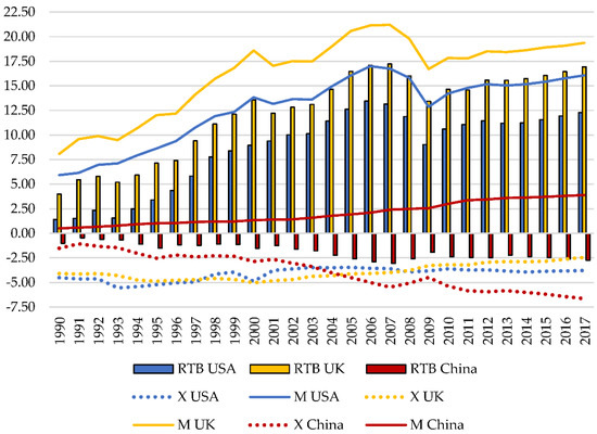
Figure 8.
PTB with indirect flows (RTB), tonnes per capita. X: exports, M: imports. Source: own elaboration based on data from Global Material Flows Database [52].
The Material Footprint, which is equivalent to the DMC from a consumption perspective, is more influenced by international trade, so the two indicators differ significantly, as shown in Figure 9.
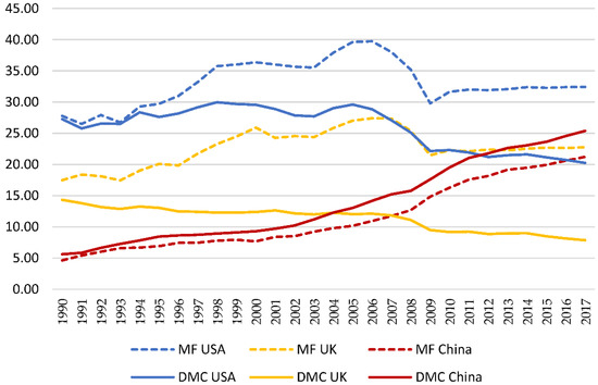
Figure 9.
DMC and Material Footprint, tonnes per capita. Source: own elaboration based on data from Global Material Flows Database [52].
The high external dependence of most rich countries means that their Material Footprint is often considerably higher than their DMC [20,29], as is the case in the USA and the United Kingdom. In contrast, China’s Material Footprint is below its DMC, as is the Material Footprint of the USA and the United Kingdom. The differences between the DMC and the Material Footprint change the efficiency levels considerably, which can be seen in Figure 10.
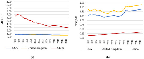
Figure 10.
(a) Material intensity, Kg/USD. (b) Material productivity, USD/kg. Source: own elaboration based on data from Global Material Flows Database [52].
Through the consumption method, the differences in efficiency between countries are more moderate, thanks to the notable decrease in efficiency in the United Kingdom and the USA and the slight improvement of China. If efficiency indicators tend to overestimate sustainability in rich countries, the production method accentuates this overestimation by relieving them of part of their environmental impact.
On the other hand, Table 3 shows how the dematerialisation ratio worsens ostensibly for the USA and, especially, for the United Kingdom. In contrast, for China the variation is minimal.
Table 3.
Decoupling ratio (1990–2017). Source: own elaboration based on data from Global Material Flows Database [52].
Graphically, no dematerialisation can be observed in any case through Material Footprint, as shown in Figure 11. Moreover, neither in the United Kingdom nor in the USA is there decoupling before the 2008 crisis, as Material Footprint growth is higher than GDP growth. The decoupling that has occurred in both countries since 2008 is probably more linked to the fall in activity and consumption because of the 2008 Crisis [10] than to major changes in material consumption patterns. In China, the differences between the DMC and the Material Footprint are very small, maintaining the decoupling, but with very high levels of material consumption growth.
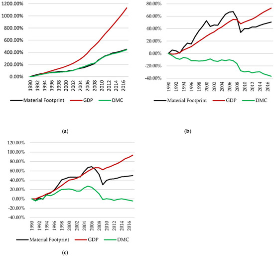
Figure 11.
(a) USA Decoupling. (b) UK decoupling. (c) China decoupling. Source: own elaboration based on data from the Global Material Flows Database [52].
From a consumption perspective, there is no evidence that economic growth coexists with a reduction in material consumption. The EKC hypotheses [4,5,7,8] are not fulfilled when this method is used to assign environmental impact, coinciding with the results of other studies focusing on the Material Footprint [18,19,40]. Table 4 summarises the main results obtained using the consumption method.
Table 4.
Summary of consumption method data, units per capita. Source: own elaboration based on data from Global Material Flows Database [52].
The evolution of the economic structure towards services and industry with a high technological content makes it possible to reduce the environmental impact on the territory itself, but at the cost of displacing activities with high material intensity to other countries. In this way, not only is the environmental impact not reduced, but it is also increased on a global scale, since relocations tend to take place to countries with less efficient production structures [25]. In this sense, China is a clear example of development through the absorption of relocations from richer countries, assuming the consequent environmental impact.
The data contained in Table A1 of Appendix A allows to check the differences between the results of each MFA method. The results for the three countries analysed can be extrapolated to most countries, except for some specific cases in which some characteristics are excessively anomalous.
4. Conclusions
In recent decades, the high impact of economic activity on nature has led to a debate about economic growth. Since the Industrial Revolution, economic growth has been closely linked to material consumption. However, there are studies that link cumulative economic growth to the evolution of the economic structure towards low material intensity activities, making it possible to decouple GDP growth from material consumption. In this paper we have analysed GDP growth and material consumption to determine the direction of their relationship in the United Kingdom, USA, and China.
From the production perspective, it has been found that in the United Kingdom and the USA there is a decoupling between the GDP growth series and the DMC, even reaching dematerialisation. In China, although there is decoupling, the DMC continues to grow strongly, which could place this country in the phase of a positive relationship between both variables, before reaching the level of development necessary for dematerialisation. Therefore, from this perspective, it is possible to affirm that the accumulation of economic growth and structural change lead to a reduction in physical requirements.
On the other hand, the consumption perspective shows a different reality. This approach allows a more complete assessment of the effects of international trade on material flows, which is very relevant in a context in which production is highly globalised. In this case, dematerialisation is not observed in any of the countries analysed. Moreover, in the United Kingdom and the USA, decoupling has only been observed since the 2008 crisis, so it could be due more to the effects of the crisis than to a real change in the structure of consumption. These countries have a very high dependence on imports of processed products, which means that from a production perspective the DMC is underestimated. This high external dependence is a consequence of the delocalisation of industrial activities that has taken place in recent decades in the rich countries, which is also behind the tertiarization of these economies. Thus, the dematerialisation that can be seen through the production approach is mainly motivated by offshoring but is rather a translation of the environmental impact. In China, the change of focus does not imply a large change in its material consumption, although it does modify its PTB significantly, because of the high indirect flows of its exports. China’s development in recent decades is closely linked to the absorption of industrial relocations from rich countries, resulting in a large physical surplus. The high economic returns obtained through this form of development have been offset by the assumption of part of the environmental impact of other countries.
Therefore, when the indirect flows associated with international trade are considered, dematerialisation does not occur, so it is not possible to decouple economic growth from material consumption. In fact, the offshoring of production implies higher material consumption to the extent that the recipient countries possess less developed technologies and imply an unnecessary increase in the transport of goods.
4.1. Policy Implications
It should be noted that the territorial or production method is the most widely used method in environmental policy making, which has consequences for its effectiveness. This method underestimates the material consumption of rich, importing countries, while overestimating that of less developed, exporting countries. The targets defined through this method are not adequately adjusted to the possibilities of each country and encourage the offshoring of material-intensive activities by rich countries. Instead, the distribution of responsibility for environmental impacts obtained through the consumption approach would make environmental policy targets more demanding for richer countries, which have a larger Material Footprint and, at the same time, the greatest capacity to act. While it is true that the consumption approach may discourage technological progress and environmental control in producer-exporter countries, this could be corrected by setting certain technological progress requirements adjusted to the level of each country. More specifically, the implications for each country would be as follows:
- In China, the production method makes it possible to check the environmental impact occurring within its borders, which is high. However, it implies taking full responsibility for it, when part of it corresponds to the production of goods that are consumed in other countries, something that should be considered when setting environmental impact reduction targets. Considering the particularities of each country, this can be extended to other economies where the export sector is predominant, especially where processed manufactures are exported;
- The United Kingdom is one of the countries that has most reduced its environmental impact over the last decades, as measured by the production method. However, a significant part of this improvement is due to the shifting of the environmental burden to other countries through offshoring. This can be verified through the consumption method, which assigns United Kingdom a considerably higher environmental impact. It is important that this is considered when setting environmental targets, to match the true capacity of each country. The United Kingdom’s situation is generalisable to many small and medium-sized Western economies with a highly developed service sector, such as much of the European Union;
- Some characteristics of the USA, such as its large size or the high prevalence of road transport, lead to a very high environmental impact per capita, even through the production method. Like the United Kingdom, the USA depends on production in other countries, to which it transfers part of its environmental burden. However, the large size of the USA means that the burden it shifts is much greater, and environmental impact reduction strategies must be adopted to avoid such burden shifts. The characteristics of the USA make it so easy to generalise its results to other countries, but, in general terms, the implications are common to most countries with high external physical dependence.
4.2. Limitations and Future Research Ampliations
One of the limitations of this work is the time span, which, due to the limited availability of data, is not long enough to cover all phases of development in each country. In addition, this research does not consider material flows that are not part of any economic process, known as hidden flows [15], so that part of the environmental impact is excluded from the analysis. It is important to note that some of the data used are estimates, so there is some margin of error.
As lines of future expansion, it would be interesting to use econometric techniques to analyse the relationships between variables, as well as to extend the time interval analysed as data availability increases. The selection of countries could also be widened, or the territorial distribution of the selected countries could be deepened. On the other hand, disaggregating material flows by category would broaden the information and improve the quality of the results.
Author Contributions
Conceptualization, P.A.-F. and R.M.R.-F.; Methodology, R.M.R.-F.; Software, P.A.-F. and R.M.R.-F.; Validation, P.A.-F. and R.M.R.-F.; Formal Analysis, P.A.-F.; Investigation, P.A.-F.; Resources, P.A.-F. and R.M.R.-F.; Data Curation, P.A.-F.; Writing–Original Draft Preparation, P.A.-F.; Writing–Review & Editing, P.A.-F. and R.M.R.-F.; Visualization, P.A.-F. and R.M.R.-F.; Supervision, P.A.-F. and R.M.R.-F.; Project Administration, P.A.-F. All authors have read and agreed to the published version of the manuscript.
Funding
This research received no external funding.
Institutional Review Board Statement
Not applicable.
Informed Consent Statement
Not applicable.
Data Availability Statement
The data presented in this study are openly available in [52].
Conflicts of Interest
The authors declare no conflict of interest.
Appendix A
Table A1.
Extension of data for the main indicators of both methods, units per capita, year 2015 1. Source: own elaboration based on data from Global Material Flows Database [52].
Table A1.
Extension of data for the main indicators of both methods, units per capita, year 2015 1. Source: own elaboration based on data from Global Material Flows Database [52].
| Country | GDP (USD 2010) | DE (Tonnes) | MF (Tonnes) | DMC (Tonnes) | RTB (Tonnes) | PTB (Tonnes) | MF-DMC |
|---|---|---|---|---|---|---|---|
| Luxembourg | 107,638.21 | 12.39 | 104.83 | 28.15 | 92.44 | 15.76 | 76.68 |
| Norway | 90,029.36 | 54.98 | 37.56 | 21.15 | −17.41 | −33.83 | 16.41 |
| Switzerland | 76,553.28 | 9.77 | 31.67 | 13.52 | 21.90 | 3.57 | 18.15 |
| Qatar | 67,443.05 | 109.15 | 14.82 | 55.23 | −94.33 | −55.03 | −40.42 |
| Ireland | 65,432.73 | 9.75 | 21.15 | 13.94 | 11.40 | 4.19 | 7.21 |
| Denmark | 60,402.13 | 14.79 | 24.34 | 16.65 | 9.54 | 1.86 | 7.68 |
| Sweden | 56,339.99 | 20.94 | 31.78 | 17.03 | 10.84 | −3.91 | 14.75 |
| Australia | 55,079.89 | 90.63 | 42.49 | 38.38 | −48.15 | −52.41 | 4.10 |
| Singapore | 54,009.74 | 5.80 | 73.28 | 33.37 | 67.48 | 27.55 | 39.91 |
| United States of America | 52,168.13 | 20.72 | 32.29 | 21.14 | 11.57 | 0.42 | 11.14 |
| Netherlands | 51,871.58 | 8.45 | 26.75 | 14.30 | 18.30 | 5.85 | 12.45 |
| Canada | 50,262.03 | 37.00 | 34.89 | 29.02 | −2.11 | −7.98 | 5.86 |
| Austria | 47,789.39 | 13.21 | 32.39 | 15.76 | 19.18 | 2.55 | 16.63 |
| Iceland | 47,533.70 | 9.94 | 34.08 | 15.20 | 24.15 | 5.03 | 18.89 |
| Japan | 47,102.58 | 4.33 | 25.02 | 9.38 | 20.70 | 5.05 | 15.64 |
| Finland | 45,647.67 | 25.88 | 35.24 | 24.61 | 9.36 | −1.27 | 10.63 |
| Belgium | 45,507.23 | 9.71 | 23.41 | 15.88 | 13.70 | 6.18 | 7.52 |
| Germany | 45,208.06 | 11.90 | 22.59 | 15.02 | 10.69 | 3.11 | 7.57 |
| United Kingdom | 42,017.14 | 6.65 | 22.71 | 8.50 | 16.07 | 1.85 | 14.22 |
| France | 41,793.54 | 9.94 | 21.19 | 11.83 | 11.24 | 1.88 | 9.36 |
| United Arab Emirates | 40,247.75 | 37.92 | 48.09 | 20.71 | 10.16 | −17.22 | 27.38 |
| New Zealand | 36,683.09 | 23.52 | 24.55 | 24.86 | 1.03 | 1.34 | −0.31 |
| Kuwait | 35,969.35 | 55.97 | 47.06 | 29.82 | −8.91 | −26.15 | 17.24 |
| Italy | 33,961.44 | 8.32 | 20.87 | 10.90 | 12.55 | 2.58 | 9.97 |
| Israel | 33,071.41 | 9.53 | 23.83 | 13.30 | 14.30 | 3.76 | 10.54 |
| Brunei Darussalam | 32,873.47 | 45.32 | 19.55 | 23.33 | −25.78 | −21.99 | −3.79 |
| Spain | 30,549.79 | 10.00 | 23.34 | 12.00 | 13.34 | 2.00 | 11.34 |
| Cyprus | 27,897.96 | 22.66 | 34.74 | 24.43 | 12.08 | 1.76 | 10.32 |
| Bahamas | 27,583.41 | 7.99 | 20.89 | 3.25 | 12.90 | −8.43 | 17.65 |
| Malta | 26,426.68 | 9.24 | 26.71 | 16.26 | 17.47 | 7.02 | 10.45 |
| South Korea | 26,063.71 | 7.97 | 27.50 | 15.90 | 19.53 | 7.93 | 11.60 |
| Slovenia | 23,826.13 | 11.16 | 23.24 | 13.77 | 12.08 | 2.61 | 9.47 |
| Greece | 22,615.39 | 10.48 | 26.18 | 11.62 | 15.69 | 1.14 | 14.55 |
| Bahrain | 22,353.36 | 26.97 | 14.68 | 28.82 | −12.29 | 1.85 | −14.15 |
| Portugal | 22,018.01 | 9.66 | 18.42 | 11.09 | 8.76 | 1.43 | 7.33 |
| Czech Republic | 21,560.83 | 15.51 | 22.53 | 17.12 | 7.02 | 1.60 | 5.41 |
| Saudi Arabia | 21,399.11 | 34.86 | 12.31 | 24.08 | −22.54 | −10.78 | −11.77 |
| Slovakia | 18,898.18 | 8.95 | 34.41 | 10.91 | 25.46 | 1.96 | 23.50 |
| Estonia | 17,633.59 | 32.44 | 27.99 | 32.98 | −4.45 | 0.53 | −4.99 |
| Trinidad and Tobago | 16,840.12 | 30.22 | 5.37 | 18.92 | −24.85 | −14.07 | −13.55 |
| Oman | 16,658.09 | 38.48 | 10.17 | 29.57 | −28.31 | −8.91 | −19.40 |
| Barbados | 15,836.38 | 2.61 | 11.10 | 2.76 | 8.48 | 0.14 | 8.33 |
| Lithuania | 15,398.86 | 12.75 | 34.87 | 14.80 | 22.11 | 2.05 | 20.06 |
| Hungary | 14,850.43 | 12.73 | 14.34 | 16.92 | 1.61 | 4.20 | −2.58 |
| Chile | 14,722.37 | 41.68 | 17.07 | 40.93 | −24.61 | −0.76 | −23.86 |
| Poland | 14,610.88 | 16.64 | 23.24 | 17.68 | 6.60 | 1.04 | 5.56 |
| Latvia | 14,414.25 | 16.01 | 21.70 | 16.00 | 5.69 | −0.01 | 5.69 |
| Croatia | 14,111.25 | 9.24 | 15.30 | 9.79 | 6.06 | 0.56 | 5.50 |
| Uruguay | 13,938.79 | 37.46 | 35.78 | 35.83 | −1.68 | −1.63 | −0.04 |
| Turkey | 13,923.68 | 16.25 | 15.60 | 17.77 | −0.65 | 1.52 | −2.17 |
| Antigua and Barbuda | 13,328.15 | 2.44 | 13.63 | 3.28 | 11.19 | 0.84 | 10.35 |
| Seychelles | 13,187.61 | 2.15 | 21.14 | 2.46 | 19.00 | 0.31 | 18.68 |
| Brazil | 11,431.15 | 18.67 | 16.43 | 16.45 | −2.24 | −2.25 | −0.02 |
| Russian Federation | 11,355.24 | 21.04 | 9.54 | 16.36 | −11.50 | −4.68 | −6.82 |
| Malaysia | 10,912.15 | 18.83 | 23.83 | 18.86 | 5.01 | 0.01 | 4.97 |
| Panama | 10,765.91 | 5.14 | 7.93 | 7.47 | 2.79 | 2.33 | 0.46 |
| Kazakhstan | 10,617.47 | 35.70 | 17.78 | 28.21 | −17.91 | −7.59 | −10.43 |
| Argentina | 10,568.16 | 16.85 | 14.29 | 15.71 | −2.56 | −1.14 | −1.42 |
| Mexico | 10,042.14 | 9.79 | 9.62 | 9.74 | −0.17 | −0.04 | −0.13 |
| Romania | 9660.43 | 11.60 | 16.41 | 11.47 | 4.80 | −0.14 | 4.94 |
| Gabon | 9521.29 | 12.77 | 5.07 | 6.77 | −7.70 | −6.00 | −1.70 |
| Mauritius | 9476.67 | 9.25 | 20.13 | 11.65 | 10.88 | 2.40 | 8.48 |
| Costa Rica | 9219.39 | 8.32 | 8.08 | 8.48 | −0.24 | 0.16 | −0.40 |
| Suriname | 8464.76 | 13.85 | 14.37 | 13.81 | 0.52 | −0.04 | 0.56 |
| Bulgaria | 7663.72 | 18.84 | 12.11 | 18.70 | −6.73 | −0.14 | −6.59 |
| Botswana | 7613.70 | 28.25 | 33.59 | 29.11 | 5.33 | 0.86 | 4.48 |
| Colombia | 7580.28 | 8.77 | 10.36 | 6.67 | 1.59 | −2.10 | 3.69 |
| South Africa | 7556.79 | 14.28 | 8.64 | 11.69 | −5.64 | −2.59 | −3.05 |
| Maldives | 7501.55 | 4.20 | 16.39 | 7.49 | 12.19 | 3.28 | 8.90 |
| Montenegro | 7286.46 | 11.18 | 24.92 | 12.78 | 13.73 | 1.59 | 12.14 |
| Turkmenistan | 6693.93 | 24.08 | 21.42 | 16.64 | −2.66 | −7.44 | 4.78 |
| Dominican Republic | 6661.87 | 5.21 | 6.55 | 5.77 | 1.33 | 0.56 | 0.77 |
| Cuba | 6522.74 | 7.36 | 8.09 | 8.16 | 0.72 | 0.80 | −0.07 |
| China | 6500.42 | 22.42 | 19.94 | 23.65 | −2.47 | 1.23 | −3.70 |
| Lebanon | 6487.90 | 7.57 | 15.35 | 10.05 | 7.78 | 2.48 | 5.30 |
| Belarus | 6384.82 | 16.13 | 0.40 | 16.60 | −15.73 | 0.47 | −16.19 |
| Namibia | 6274.75 | 10.85 | 8.16 | 11.02 | −2.69 | 0.17 | −2.86 |
| Serbia | 6157.25 | 14.03 | 19.72 | 14.27 | 5.69 | 0.23 | 5.46 |
| Peru | 6114.23 | 15.55 | 9.38 | 15.14 | −6.17 | −0.44 | −5.76 |
| Iran | 6070.19 | 15.34 | 13.83 | 14.44 | −1.51 | −0.91 | −0.61 |
| Azerbaijan | 6063.72 | 12.53 | 5.85 | 8.42 | −6.68 | −4.10 | −2.58 |
| Libya | 5899.90 | 11.40 | 3.80 | 10.81 | −7.60 | −0.59 | −7.01 |
| Thailand | 5741.35 | 11.78 | 14.43 | 12.30 | 2.64 | 0.52 | 2.12 |
| Bosnia and Herzegovina | 5352.72 | 11.36 | 8.79 | 11.94 | −2.57 | 0.59 | −3.15 |
| Ecuador | 5330.54 | 10.14 | 10.70 | 9.09 | 0.56 | −1.05 | 1.61 |
| Iraq | 5295.99 | 9.09 | 2.75 | 6.25 | −6.34 | −2.84 | −3.50 |
| Guyana | 5257.46 | 25.25 | 116.73 | 24.74 | 91.49 | −0.51 | 92.00 |
| Macedonia | 5105.40 | 12.50 | 13.28 | 13.94 | 0.77 | 1.44 | −0.66 |
| Paraguay | 4944.19 | 13.36 | 14.64 | 12.15 | 1.28 | −1.22 | 2.49 |
| Algeria | 4775.87 | 9.91 | 3.04 | 8.72 | −6.87 | −1.19 | −5.68 |
| Jamaica | 4722.05 | 8.26 | 8.26 | 7.13 | 0.00 | −1.14 | 1.14 |
| Albania | 4524.37 | 9.41 | 10.86 | 9.70 | 1.45 | 0.22 | 1.16 |
| Fiji Islands | 4352.47 | 6.28 | 7.21 | 6.86 | 0.93 | 0.58 | 0.35 |
| Tunisia | 4308.42 | 8.52 | 6.21 | 9.20 | −2.31 | 0.68 | −2.99 |
| Belize | 4300.56 | 12.03 | 7.95 | 11.98 | −4.09 | −0.05 | −4.03 |
| Georgia | 4185.81 | 4.86 | 8.47 | 6.25 | 3.61 | 1.39 | 2.22 |
| Armenia | 3923.72 | 9.09 | 7.37 | 9.99 | −1.72 | 0.90 | −2.62 |
| Mongolia | 3895.41 | 40.19 | 13.29 | 33.49 | −26.90 | −6.70 | −20.21 |
| Indonesia | 3824.27 | 8.61 | 6.02 | 7.19 | −2.59 | −1.42 | −1.17 |
| Angola | 3748.32 | 8.52 | 3.75 | 5.42 | −4.77 | −3.11 | −1.67 |
| Sri Lanka | 3647.39 | 4.42 | 3.93 | 5.36 | −0.49 | 0.94 | −1.43 |
| Samoa | 3558.12 | 4.68 | 7.61 | 5.13 | 2.93 | 0.45 | 2.48 |
| Cape Verde | 3414.56 | 5.84 | 8.50 | 6.74 | 2.67 | 0.91 | 1.76 |
| Jordan | 3350.39 | 8.59 | 8.18 | 9.52 | −0.40 | 0.93 | −1.34 |
| El Salvador | 3314.70 | 4.81 | 6.31 | 5.43 | 1.50 | 0.61 | 0.88 |
| Morocco | 3222.05 | 7.04 | 3.83 | 7.66 | −3.21 | 0.62 | −3.84 |
| Guatemala | 3210.87 | 6.42 | 3.82 | 6.54 | −2.60 | 0.11 | −2.72 |
| Rep Congo | 3097.28 | 6.10 | 2.39 | 3.81 | −3.71 | −2.29 | −1.42 |
| Moldova | 2953.72 | 7.61 | 3.54 | 8.26 | −4.07 | 0.65 | −4.72 |
| Ukraine | 2828.89 | 13.97 | 11.35 | 11.80 | −2.62 | −2.16 | −0.46 |
| Vanuatu | 2781.79 | 6.01 | 7.47 | 6.04 | 1.46 | 0.03 | 1.43 |
| Bhutan | 2780.82 | 12.86 | 10.22 | 10.25 | −2.64 | −2.63 | −0.03 |
| Philippines | 2735.19 | 4.14 | 4.37 | 3.97 | 0.23 | −0.19 | 0.39 |
| Egypt | 2704.92 | 7.03 | 4.88 | 7.61 | −2.15 | 0.58 | −2.72 |
| Nigeria | 2549.72 | 4.06 | 2.73 | 3.49 | −1.34 | −0.57 | −0.76 |
| Bolivia | 2361.06 | 13.94 | 5.39 | 12.56 | −8.55 | −1.38 | −7.17 |
| Papua New Guinea | 2336.81 | 9.54 | 2.73 | 10.95 | −6.81 | 1.41 | −8.22 |
| Uzbekistan | 2138.57 | 9.51 | 6.14 | 9.28 | −3.37 | −0.23 | −3.14 |
| Honduras | 2067.29 | 5.56 | 4.37 | 5.69 | −1.19 | 0.05 | −1.32 |
| Nicaragua | 1836.01 | 6.13 | 4.20 | 6.47 | −1.93 | 0.34 | −2.27 |
| Sudan | 1825.72 | 4.45 | 4.36 | 4.63 | −0.09 | 0.19 | −0.27 |
| India | 1751.66 | 5.05 | 4.45 | 5.34 | −0.59 | 0.29 | −0.88 |
| Mauritania | 1732.59 | 10.06 | 2.59 | 7.52 | −7.47 | −2.54 | −4.93 |
| Vietnam | 1667.17 | 13.52 | 11.79 | 13.59 | −1.73 | 0.08 | −1.80 |
| Zambia | 1641.01 | 8.04 | 3.39 | 8.07 | −4.65 | 0.03 | −4.68 |
| Ghana | 1625.91 | 6.58 | 3.56 | 6.84 | −3.02 | 0.26 | −3.28 |
| Laos | 1538.85 | 10.76 | 6.60 | 10.61 | −4.16 | −0.16 | −4.00 |
| Cote d’Ivoire | 1463.71 | 2.94 | 0.98 | 3.08 | −1.96 | 0.14 | −2.09 |
| Cameroon | 1441.78 | 3.93 | 1.87 | 4.03 | −2.05 | 0.11 | −2.16 |
| Senegal | 1384.52 | 3.04 | 2.42 | 3.21 | −0.62 | 0.17 | −0.79 |
| Lesotho | 1363.93 | 11.61 | 11.48 | 11.82 | −0.14 | 0.21 | −0.34 |
| Myanmar | 1335.20 | 3.43 | 1.35 | 3.30 | −2.08 | −0.13 | −1.95 |
| Haiti | 1260.60 | 1.39 | 1.34 | 1.59 | −0.05 | 0.20 | −0.25 |
| Zimbabwe | 1234.10 | 3.47 | 3.42 | 3.59 | −0.05 | 0.12 | −0.17 |
| Sao Tome and Principe | 1232.17 | 3.01 | 6.04 | 3.37 | 3.03 | 0.35 | 2.67 |
| Benin | 1129.00 | 4.62 | 4.28 | 5.01 | −0.34 | 0.38 | −0.73 |
| Kenya | 1093.13 | 3.05 | 3.07 | 3.28 | 0.02 | 0.22 | −0.20 |
| Pakistan | 1081.29 | 4.19 | 3.16 | 4.43 | −1.03 | 0.24 | −1.27 |
| Cambodia | 1024.62 | 4.33 | 3.38 | 4.88 | −0.95 | 0.55 | −1.50 |
| Kyrgyzstan | 1021.16 | 7.33 | 8.52 | 8.20 | 1.19 | 0.88 | 0.31 |
| Bangladesh | 1002.39 | 2.35 | 2.28 | 2.58 | −0.06 | 0.23 | −0.29 |
| Chad | 956.66 | 2.57 | 1.59 | 2.59 | −0.98 | 0.02 | −1.00 |
| Tajikistan | 936.00 | 3.04 | 3.55 | 3.37 | 0.52 | 0.34 | 0.18 |
| Uganda | 903.85 | 2.98 | 2.63 | 3.03 | −0.35 | 0.05 | −0.40 |
| Tanzania | 872.00 | 3.22 | 1.44 | 3.35 | −1.78 | 0.13 | −1.91 |
| Yemen | 785.34 | 1.92 | 1.09 | 2.23 | −0.83 | 0.31 | −1.14 |
| Rwanda | 764.62 | 2.80 | 3.04 | 2.87 | 0.25 | 0.07 | 0.18 |
| Gambia | 754.99 | 2.24 | 2.29 | 2.47 | 0.05 | 0.23 | −0.18 |
| Guinea | 750.40 | 5.05 | 2.21 | 3.64 | −2.84 | −1.41 | −1.43 |
| Nepal | 732.00 | 3.55 | 2.70 | 3.79 | −0.85 | 0.25 | −1.09 |
| South Sudan | 730.93 | 1.38 | 1.26 | 0.78 | −0.12 | −0.84 | 0.48 |
| Mali | 729.63 | 5.56 | 4.55 | 5.69 | −1.01 | 0.12 | −1.13 |
| Burkina Faso | 726.71 | 4.16 | 3.82 | 4.27 | −0.33 | 0.11 | −0.44 |
| Togo | 630.94 | 4.22 | 2.57 | 4.25 | −1.64 | 0.00 | −1.68 |
| Mozambique | 580.05 | 2.49 | 1.93 | 2.41 | −0.56 | −3.96 | −0.47 |
| Afghanistan | 574.18 | 1.86 | 1.28 | 2.00 | −0.58 | 0.15 | −0.72 |
| Liberia | 571.45 | 3.22 | 1.69 | 3.29 | −1.53 | 0.07 | −1.60 |
| Niger | 520.76 | 3.43 | 3.26 | 3.49 | −0.16 | 0.06 | −0.22 |
| Malawi | 507.55 | 3.34 | 1.22 | 3.36 | −2.12 | 0.02 | −2.14 |
| Ethiopia | 482.64 | 2.94 | 0.70 | 3.02 | −2.24 | 0.08 | −2.32 |
| Madagascar | 469.94 | 2.28 | 0.83 | 2.40 | −1.46 | 0.12 | −1.58 |
| Sierra Leone | 441.14 | 6.53 | 5.93 | 6.41 | −0.59 | −0.38 | −0.47 |
| DR Congo | 411.02 | 2.30 | 2.03 | 2.33 | −0.28 | 0.03 | −0.30 |
| Central African Republic | 346.69 | 3.08 | 2.33 | 3.10 | −0.75 | 0.02 | −0.77 |
| Burundi | 228.43 | 1.62 | 1.50 | 1.66 | −0.13 | 0.04 | −0.16 |
1 Data from 2015 is used because it is the most recent year for which data is available for most countries.
References
- Naredo, J.M. Economía y Sostenibilidad. La Economía Ecológica En Perspectiva. POLIS Rev. Latinoam. 2001, 1, 27. [Google Scholar]
- Meadows, D.H.; Meadows, D.L.; Randers, J.; Behrens, W.W., III. The Limits to Growth. A Report for The Club of Rome’s Project on the Predicament of Mankind; Universe Books: New York, NY, USA, 1972. [Google Scholar]
- United Nations. Report of the World Commission on Environment and Development: Our Common Future; United Nations: New York, NY, USA, 1987. [Google Scholar]
- Shafik, N.; Bandyopadhyay, S. Ecomomic Growth and Enivronmental Quality, Time Series Anda Cross-Country Evidence; World Development Report; World Bank Group: Washington, DC, USA, 1992. [Google Scholar]
- Panayotou, T. Environmental Degradation at Different Stages of Economic Development. In Beyond Rio; Ahmed, I., Doeleman, J.A., Eds.; Palgrave Macmillan: London, UK, 1995; pp. 13–36. [Google Scholar]
- Castells, M. La Era de La Información; Alianza: Madriz, Nicaragua, 1997. [Google Scholar]
- Aruga, K. Investigating the Energy-Environmental Kuznets Curve Hypothesis for the Asia-Pacific Region. Sustainability 2019, 11, 2395. [Google Scholar] [CrossRef]
- Maneejuk, N.; Ratchakom, S.; Maneejuk, P.; Yamaka, W. Does the Environmental Kuznets Curve Exist? An International Study. Sustainability 2020, 12, 9117. [Google Scholar] [CrossRef]
- Scheel, C.; Aguiñaga, E.; Bello, B. Decoupling Economic Development from the Consumption of Finite Resources Using Circular Economy. A Model for Developing Countries. Sustainability 2020, 12, 1291. [Google Scholar] [CrossRef]
- Shao, Q.; Schaffartzik, A.; Mayer, A.; Krausmann, F. The High ‘Price’ of Dematerialization: A Dynamic Panel Data Analysis of Material Use and Economic Recession. J. Clean. Prod. 2017, 167, 120–132. [Google Scholar] [CrossRef]
- Bampatsou, C.; Halkos, G.; Dimou, A. Determining Economic Productivity under Environmental and Resource Pressures: An Empirical Application. J. Econ. Struct. 2017, 6, 12. [Google Scholar] [CrossRef]
- Cohen, G.; Jalles, J.T.; Loungani, P.; Marto, R. The Long-Run Decoupling of Emissions and Output: Evidence from the Largest Emitters. Energy Policy 2018, 118, 58–68. [Google Scholar] [CrossRef]
- Steinberger, J.K.; Krausmann, F.; Getzner, M.; Schandl, H.; West, J. Development and Dematerialization: An International Study. PLoS ONE 2013, 8, e70385. [Google Scholar] [CrossRef]
- Martínez-Alier, J.; Pascual, U.; Vivien, F.-D.; Zaccai, E. Sustainable De-Growth: Mapping the Context, Criticisms and Future Prospects of an Emergent Paradigm. Ecol. Econ. 2010, 69, 1741–1747. [Google Scholar] [CrossRef]
- Adriaanse, A. Resource Flows: The Material Basis of Industrial Economies; World Resources Institute: Washington, DC, USA, 1997. [Google Scholar]
- Bithas, K.; Kalimeris, P. Unmasking Decoupling: Redefining the Resource Intensity of the Economy. Sci. Total Environ. 2018, 619–620, 338–351. [Google Scholar] [CrossRef]
- Steinberger, J.K.; Krausmann, F. Material and Energy Productivity. Policy Anal. 2011, 45, 1169–1176. [Google Scholar] [CrossRef]
- Schandl, H.; Fischer-Kowalski, M.; West, J.; Giljum, S.; Dittrich, M.; Eisenmenger, N.; Geschke, A.; Lieber, M.; Wieland, H.; Schaffartzik, A.; et al. Global Material Flows and Resource Productivity: Forty Years of Evidence: Global Material Flows and Resource Productivity. J. Ind. Ecol. 2018, 22, 827–838. [Google Scholar] [CrossRef]
- Wiedmann, T.O.; Schandl, H.; Lenzen, M.; Moran, D.; Suh, S.; West, J.; Kanemoto, K. The Material Footprint of Nations. Proc. Natl. Acad. Sci. USA 2015, 112, 6271–6276. [Google Scholar] [CrossRef] [PubMed]
- Carpintero, Ó. Los costes ambientales del sector servicios y la nueva economía: Entre la desmaterialización y el efecto rebote. Econ. Ind. 2003, 352, 59–76. [Google Scholar]
- Carpintero, Ó. Pautas de consumo, desmaterialización y ‘nueva economía’: Entre la realidad y el deseo. In Necesidades, Consumo y Sostenibilidad; Colección Urbanitats; CCCB/Bakeaz: Barcelona, Spain, 2003. [Google Scholar]
- Pothen, F.; Schymura, M. Bigger Cakes with Fewer Ingredients? A Comparison of Material Use of the World Economy. Ecol. Econ. 2015, 109, 109–121. [Google Scholar] [CrossRef]
- Krausmann, F.; Schandl, H.; Eisenmenger, N.; Giljum, S.; Jackson, T. Material Flow Accounting: Measuring Global Material Use for Sustainable Development. Annu. Rev. Environ. Resour. 2017, 42, 647–675. [Google Scholar] [CrossRef]
- Arto, I.; Roca, J.; Serrano, M. Emisiones territoriales y fuga de emisiones. Análisis del caso español. Rev. Iberoam. Econ. Ecol. 2012, 18, 73–87. [Google Scholar]
- Dittrich, M.; Giljum, S.; Lutter, S.; Polzin, C. Green Economies around the World? Implications of Resource Use for Development and the Environment; Sustainable Europe Research Institute (SERI): Vienna, Austria, 2012. [Google Scholar]
- Knight, K.W.; Schor, J.B. Economic Growth and Climate Change: A Cross-National Analysis of Territorial and Consumption-Based Carbon Emissions in High-Income Countries. Sustainability 2014, 6, 3722–3731. [Google Scholar] [CrossRef]
- Eisenmenger, N.; Giljum, S.; Lutter, S.; Marques, A.; Theurl, M.; Pereira, H.; Tukker, A. Towards a Conceptual Framework for Social-Ecological Systems Integrating Biodiversity and Ecosystem Services with Resource Efficiency Indicators. Sustainability 2016, 8, 201. [Google Scholar] [CrossRef]
- Ayres, R.U.; Kneese, A.V. Production, Consumption, and Externalities. Am. Econ. Rev. 1969, 59, 282–297. [Google Scholar]
- Ayres, R.U.; Ayres, L. Accounting for Resources: Economy-Wide Applications of Mass-Balance Principles to Materials and Waste; Edward Elgar: Camberley, UK, 1998. [Google Scholar]
- Daniels, P.L.; Moore, S. Approaches for Quantifying the Metabolism of Physical Economies: Part I: Methodological Overview. J. Ind. Ecol. 2001, 5, 69–93. [Google Scholar] [CrossRef]
- Daniels, P.L. Approaches for Quantifying the Metabolism of Physical Economies: A Comparative Survey: Part II: Review of Individual Approaches. J. Ind. Ecol. 2002, 6, 65–88. [Google Scholar] [CrossRef]
- Steurer, A.; Schutz, H. Economy-Wide Material Flow Accounts and Derived Indicators: A Methodological Guide; Eurostat, Ed.; Office for Official Publications of the European Communities: Luxembourg, 2001. [Google Scholar]
- Fischer-Kowalski, M.; Krausmann, F.; Giljum, S.; Lutter, S.; Mayer, A.; Bringezu, S.; Moriguchi, Y.; Schütz, H.; Schandl, H.; Weisz, H. Methodology and Indicators of Economy-Wide Material Flow Accounting. J. Ind. Ecol. 2011, 15, 855–876. [Google Scholar] [CrossRef]
- EUROSTAT. Economy-Wide Material Flow Accounts Handbook: 2018 Edition; Publications Office of the European Union: Luxembourg, 2018. [Google Scholar]
- Fischer-Kowalski, M.; Haberl, H. Sustainable Development: Socio-economic Metabolism and Colonization of Nature. Int. Soc. Sci. J. 1998, 50, 573–587. [Google Scholar] [CrossRef]
- Ayres, R.U.; Simonis, U.E. Industrial Metabolism: Restructuring for Sustainable Development; United Nations University Press: New York, NY, USA, 1994. [Google Scholar]
- Fischer-Kowalski, M.; Weisz, H. Society as Hybrid between Material and Symbolic Realms: Toward a Theoretical Framework of Society-Nature Interaction. Adv. Hum. Ecol. 1999, 8, 215–251. [Google Scholar]
- Georgescu-Roegen, N. La Ley de Entropía y El Proceso Económico; Fundación Argentaria: Madrid, Spain, 1996. [Google Scholar]
- Piñero, P.; Bruckner, M.; Wieland, H.; Pongrácz, E.; Giljum, S. The Raw Material Basis of Global Value Chains: Allocating Environmental Responsibility Based on Value Generation. Econ. Syst. Res. 2019, 31, 206–227. [Google Scholar] [CrossRef]
- Schandl, H.; Fischer-Kowalski, M.; West, J.; Giljum, S.; Dittrich, M.; Eisenmenger, N.; Geschke, A.; Lieber, M.; Wieland, H.; Schaffartzik, A.; et al. Global Material Flows and Resource Productivity, Assessment Study for the UNEP International Resource Panel; United Nations Environment Programme: Paris, France, 2016. [Google Scholar]
- Schaffartzik, A.; Wiedenhofer, D.; Eisenmenger, N. Raw Material Equivalents: The Challenges of Accounting for Sustainability in a Globalized World. Sustainability 2015, 7, 5345–5370. [Google Scholar] [CrossRef]
- Carpintero, Ó. El Metabolismo Económico Regional Español: Glosario de Términos; FUHEM Ecosocial: Madrid, Spain, 2015. [Google Scholar]
- Anke Schaffartzik; Melanie Pichler Extractive Economies in Material and Political Terms: Broadening the Analytical Scope. Sustainability 2017, 9, 1047. [CrossRef]
- Eisenmenger, N.; Fischer-Kowalski, M.; Weisz, H. Indicators of natural resource use and consumption. In Sustainability Indicators; SCOPE: Washington, DC, USA, 2007; pp. 193–211. [Google Scholar]
- UNEP. Decoupling Natural Resource Use and Environmental Impacts from Economic Growth; UNEP: Nairobi, Kenya, 2011. [Google Scholar]
- Fischer-Kowalski, M.; Haberl, H. Social metabolism: A metric for biophysical growth and degrowth. In Handbook of Ecological Economics; Edward Elgard: Cheltenham, UK, 2015; pp. 100–138. [Google Scholar]
- Ruffing, K. Indicators to measure decoupling of environmental pressure from economic growth. In Sustainability Indicators: A Scientific Assessment; SCOPE: Washington, DC, USA, 2007; pp. 221–223. [Google Scholar]
- Giljum, S.; Hak, T.; Hinterberger, F.; Kovanda, J. Environmental Governance in the European Union: Strategies and Instruments for Absolute Decoupling. Int. J. Sustain. Dev. 2005, 8, 31. [Google Scholar] [CrossRef]
- Martínez-Alier, J. Los Conflictos Ecológico-Distributivos y Los Indicadores de Sustentabilidad. Rev. Iberoam. Econ. Ecol. 2004, 1, 21–30. [Google Scholar]
- UNEP. Assessing the Environmental Impacts of Consumption and Production. Int. J. Sustain. High. Educ. 2010, 11. [Google Scholar] [CrossRef]
- Dittrich, M.; Bringezu, S.; Schütz, H. The Physical Dimension of International Trade, Part 2: Indirect Global Resource Flows between 1962 and 2005. Ecol. Econ. 2012, 79, 32–43. [Google Scholar] [CrossRef]
- United Nations Environment Programme International Resource Panel Global Material Flows Database. Available online: https://www.resourcepanel.org/global-material-flows-database (accessed on 1 March 2021).
- Weisz, H.; Krausmann, F.; Amann, C.; Eisenmenger, N.; Erb, K.-H.; Hubacek, K.; Fischer-Kowalski, M. The Physical Economy of the European Union: Cross-Country Comparison and Determinants of Material Consumption. Ecol. Econ. 2006, 58, 676–698. [Google Scholar] [CrossRef]
- Fernández-Herrero, L.; Duro, J.A. What Causes Inequality in Material Productivity between Countries? Ecol. Econ. 2019, 162, 1–16. [Google Scholar] [CrossRef]
- Palazuelos, E.; Machín, A. Ruidos y Silencios de La Política Energética de Estados Unidos. Econ. UNAM 2008, 14, 7–36. [Google Scholar]
- Bradshaw, C.J.A.; Giam, X.; Sodhi, N.S. Evaluating the Relative Environmental Impact of Countries. PLoS ONE 2010, 5, e10440. [Google Scholar] [CrossRef]
- Palazuelos, E.; García, C. La Transición Energética en China. Rev. Econ. Mund. 2008, 20, 165–196. [Google Scholar]
- Pérez Lagüela, E. El metabolismo de la economía china. Una visión del desarrollo desde la Economía ecológica. Rev. Econ. Mund. 2017. [Google Scholar] [CrossRef]
- Levy, D. Offshoring in the New Global Political Economy. J. Manag. Stud. 2005, 685–693. [Google Scholar] [CrossRef]
- Santarcángelo, J.; Schteingart, D.; Porta, F. Cadenas Globales de Valor: Una mirada crítica a una nueva forma de pensar el desarrollo. Cuad. Econ. Crítica 2017, 4, 99–129. [Google Scholar]
- Álvarez, N.; Medialdea, B. Revista de Economía Mundial; Universidad Huelva: Huelva, Spain, 2010; pp. 165–191. [Google Scholar]
- Palomo Garrido, A. Desarrollo y consecuencias de la globalización financiera. Nómadas Rev. Crítica Cienc. Soc. Juríd. 2013, 35, 353–373. [Google Scholar] [CrossRef]
- Carpintero, Ó.; Naredo, J.M. Sobre Financiarización y Neoextractivismo. Papeles Relac. Ecosociales 2018, 143, 97–108. [Google Scholar]
- Salvador, A.I. El proceso de apertura de la economía china a la inversión extranjera. Rev. Econ. Mund. 2012, 30, 209–231. [Google Scholar]
- Salvador, A.I. El proceso de reforma económica de China y su adhesión a la OMC. Pecvnia Rev. Fac. Cienc. Económicas Empres. Univ. 2008, 7, 257–284. [Google Scholar] [CrossRef]
- Bustelo, P.; Fernández Lommen, Y. Gradualismo y factores estructurales en la reforma económica china (1978–1995). Doc. Trab. Fac. Cienc. Económicas Empres. 1996, 11, 1–28. [Google Scholar]
- Claro, S. 25 años de reformas económicas en China: 1978–2003. Cuad. Inf. Econ. 2003, 186, 74–81. [Google Scholar]
- Bustelo, P. China 2006–2010: ¿Hacia una Nueva Pauta de Desarrollo? Real Instituto Elcano de Estudios Internacionales y Estratégicos: Madrid, Spain, 2005. [Google Scholar]
- Lommen, Y.F. El futuro incierto de China. Retos del duodécimo Plan Quinquenal. Estud. Política Exter. 2011, 56, 46–54. [Google Scholar]
- Pérez, Á.P. Boletín del Instituto Español de Estudios Estratégicos; Publicaciones Defensa: Madrid, Spain, 2016; pp. 709–724. [Google Scholar]
- Bustillo, I.; Artecona, R.; Makhoul, I.; Perrotti, D. Energía y Políticas Públicas en Estados Unidos. Una Relación Virtuosa Para El Desarrollo de Fuentes No Convencionales; CEPAL: Santiago, Chile, 2015. [Google Scholar]
- Hudson, R.; Sadler, D. State Policies and the Changing Geography of the Coal Industry in the United Kingdom in the 1980s and 1990s. Trans. Inst. Br. Geogr. 1990, 15, 435–454. [Google Scholar] [CrossRef]
- Xun, S. Minerals Yearbook: The Mineral Industry of China; USGS: Washington, DC, USA, 2018.
- Bruckner, M.; Giljum, S.; Lutz, C.; Wiebe, K.S. Materials Embodied in International Trade—Global Material Extraction and Consumption between 1995 and 2005. Glob. Environ. Chang. 2012, 22, 568–576. [Google Scholar] [CrossRef]
- Piñero, P.; Pérez-Neira, D.; Infante-Amate, J.; Chas-Amil, M.L.; Doldán-García, X.R. Unequal Raw Material Exchange between and within Countries: Galicia (NW Spain) as a Core-Periphery Economy. Ecol. Econ. 2020, 172, 106621. [Google Scholar] [CrossRef]
- Muñoz, P.; Giljum, S.; Roca, J. The Raw Material Equivalents of International Trade. J. Ind. Ecol. 2009, 13, 881–897. [Google Scholar] [CrossRef]
- Chen, X.; Mao, J.; Tian, H. Analysis of China’s Iron Trade Flow: Quantity, Value and Regional Pattern. Sustainability 2020, 12, 10427. [Google Scholar] [CrossRef]
- Huang, J. The Prospects for China’s Food Security and Imports: Will China Starve the World via Imports? J. Integr. Agric. 2017, 16, 2933–2944. [Google Scholar] [CrossRef]


Publisher’s Note: MDPI stays neutral with regard to jurisdictional claims in published maps and institutional affiliations. |
© 2021 by the authors. Licensee MDPI, Basel, Switzerland. This article is an open access article distributed under the terms and conditions of the Creative Commons Attribution (CC BY) license (https://creativecommons.org/licenses/by/4.0/).