Exploring the Impact of Climate and Extreme Weather on Fatal Traffic Accidents

Abstract

Climate change and the extreme weather have a negative impact on road traffic safety, resulting in severe road traffic accidents. In this study, a negative binomial model and a log-change model are proposed to analyse the impact of various factors on fatal traffic accidents. The dataset used in this study includes the fatal traffic accident frequency, social development indicators and climate indicators in California and Arizona. The results show that both models can provide accurate fitting results. Climate variables (i.e., average temperature and standard precipitation 24) can significantly affect the frequency of fatal traffic accidents. Non-climate variables (i.e., beer consumption, rural Vehicle miles travelled ratio, and vehicle performance) also have a significant impact. The modelling results can provide decision-making guidelines for the transportation management agencies to improve road traffic safety.

1. Introduction

Traffic accidents can result in considerable losses to individuals and society. According to the World Health Organization (WHO), globally road traffic accidents cause approximately 1.35 million deaths annually and cost $518 billion USD. Without suitable improvement strategies, road traffic injuries are expected to become the fifth leading cause of death by 2030. Thus, it is necessary to analyse the influential factors affecting traffic accidents in order to improve the traffic safety. There are a large number of factors affecting road traffic accidents in the existing literature, such as economy, climate, and traffic safety laws.

Some research shows that economic growth is significantly related to the increase of road traffic accidents [1,2,3,4]. Among the economic factors, the impact of GDP and residents’ income are more significant. The increase of GDP and per capita income result in higher traffic accident mortality. Some studies [5,6,7] have examined the impact of fuel prices and fuel taxes on traffic accidents. In addition, studies [8,9,10] have investigated the relationship between various social development indicators and road traffic accidents. It has been observed that the Gini index, average household income and road network distribution have impacts on road traffic accident mortality. The reduction of traffic volume, young drivers and drunk driving can significantly reduce the number of traffic deaths. Moreover, the proportion of high capacity roads, unemployment rate, and motorization rate can reduce the number of traffic deaths and serious injuries.

Some studies have examined the impact of weather factors on traffic accidents [11,12,13,14,15,16,17,18,19], but there are few studies focused on the impact of climate factors on fatal traffic accidents from the macro perspective. Climate change can influence road environment and driving behaviour, which in turn affect the risk of road traffic accidents [20,21,22,23]. The climatic factors affecting the traffic accident include temperature, precipitation and wind. Temperature has an influence on the risk level of road traffic accidents, especially the extreme low temperature conditions and the hot weather [24,25,26,27,28,29]. Extreme cold weather and icy roads will significantly increase the frequency of traffic accidents, especially those accidents caused by vehicle skidding. Also, rainfall and other characteristics can affect the risk of traffic accidents [30,31,32,33,34]. The road traffic accident rate in rainy days is significantly higher than that in sunny days. Rainfall can also increase the rate of traffic accident casualties, and the impact of rainy weather changes with the amount of rainfall. In addition, the impact of windy weather on road traffic accidents cannot be ignored. The occurrence of windy weather will increase the risk of traffic accidents [35,36]. In stormy weather, when the gust speed is higher than a certain threshold, the probability of traffic accidents increases accordingly. Strong winds increase the frequency of rollovers, sideslip and spin, especially rollovers [37].

The existing traffic safety law studies mainly consider Driving Under the Influence (DUI), safety belts, helmets (for motocyclists) and so on. Revision of DUI laws and the increase of the legal drinking age can reduce traffic accidents and casualties [38,39]. The improvement of DUI law can significantly reduce the incidence of alcohol related traffic accidents. Moreover, the increase of legal drinking age can also reduce the frequency of drunk driving, thereby reducing road traffic accidents. There are also some studies focusing on the possible impact of safety belt and helmet use laws, which show that relevant laws can have a certain impact on motor vehicle traffic accidents [40,41,42].The results show that the abolition of safety belt law may lead to a significant increase in the number of traffic casualties.

Two issues have not been adequately addressed in the previous research. First, these studies fail to comprehensively investigate the influence of economy, climate and law so that they ignore the overall effect. The second point is that most studies adopt simple mathematical statistical methods in analyzing the impact of climate or law, which cannot accurately explore the sensitivity of influencing factors to traffic accidents. The objective of this paper is to comprehensively explore the impact of climate and other factors on fatal traffic accident from a macroscopic perspective. And the influence of these factors on the frequency of fatal traffic accidents can be quantified, especially the climate factors. Furthermore, this paper explains the influence mechanism of these factors on fatal traffic accidents.

The next section introduces the data characteristics. The third section describes the data process procedure and statistical analysis. The fourth section shows the modelling results, and discussions. The last section provides the conclusions.

2. Data Description

The dataset used in this study integrates multi-source data [43,44,45] from California and Arizona (USA) for time period 2001 to 2016. The original dataset may be divided into three main categories: fatal traffic accidents, social development and climate characteristics. Social development variables include economy, traffic, laws and regulations and other factors indicating social conditions. Such factors usually affect residents’ activities and traffic conditions. Climate characteristics include temperature, precipitation and humidity, meteorological disasters, and other factors reflecting the regional climate characteristics. These factors usually affect the driving environment and the physical and mental state of drivers.

2.1. Fatal Traffic Accident Data

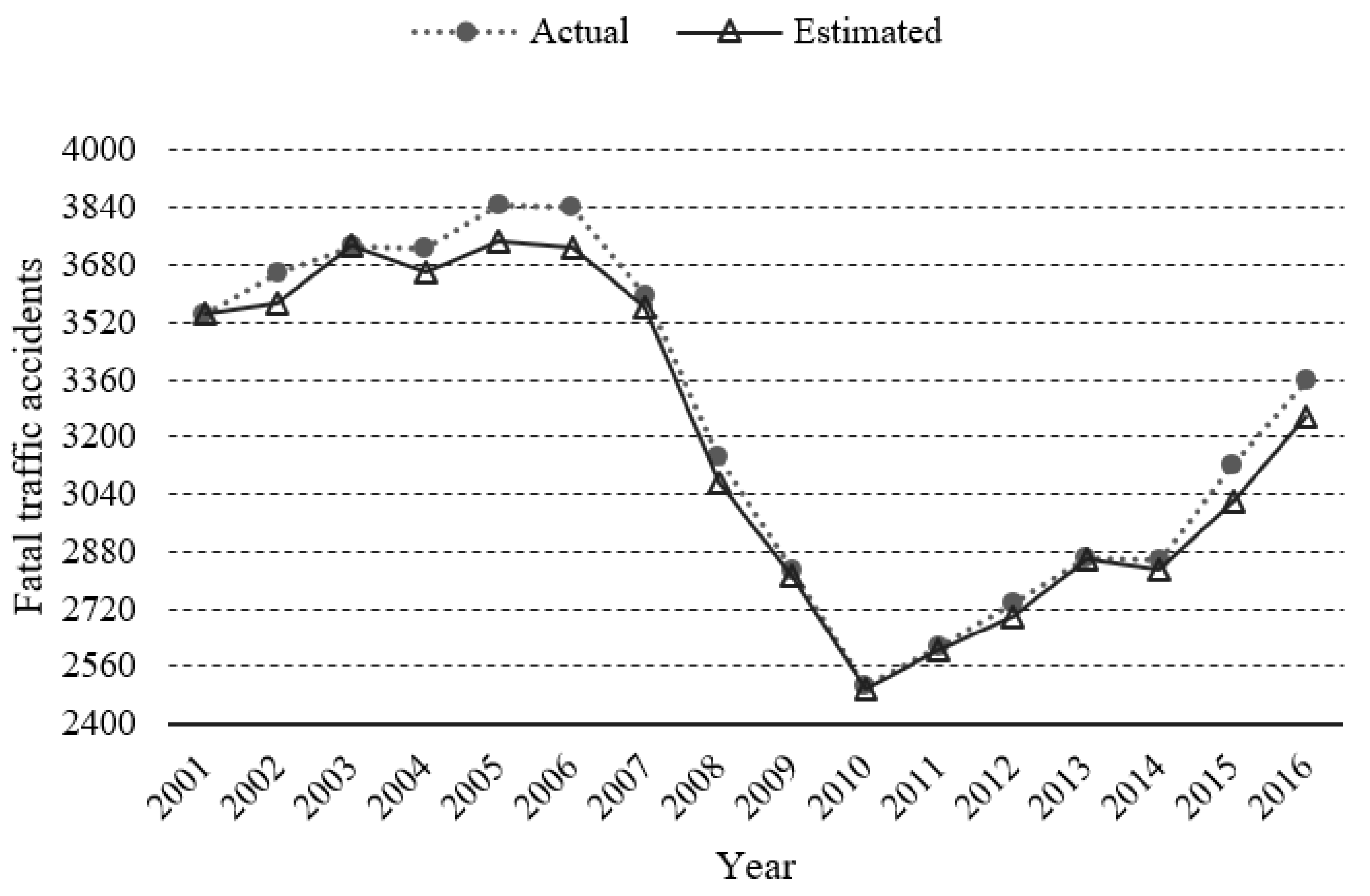
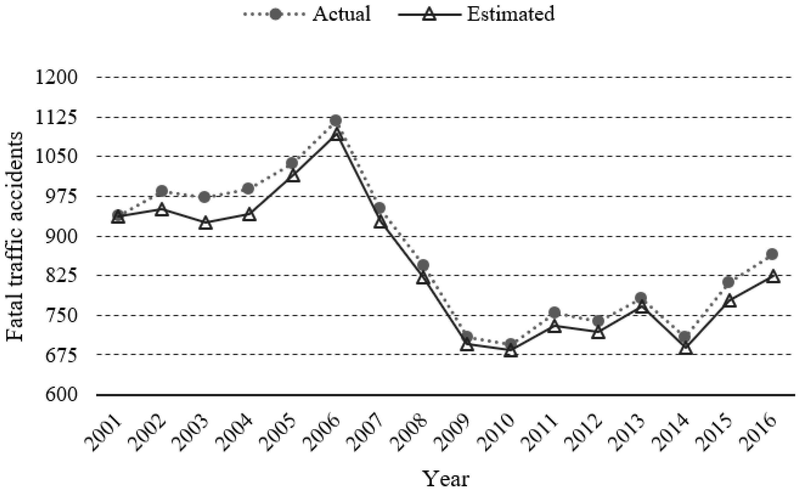
The fatal traffic accident data used in this study are obtained from the Fatality Analysis Reporting System (FARS) of the National Highway Traffic Safety Administration (NHTSA). Figure 1 shows the trend of fatal traffic accidents in California and Arizona from 2001 to 2016 respectively. The time span of the collected traffic accident frequency is a year, and the space span is a state.

The trend of fatal traffic accidents in California can be summarized into three periods. First, the frequency of fatal traffic accidents shows a slow upward trend from 3543 in 2001 to 3839 in 2006. Second, the fatal traffic accident frequency shows a sharp downward trend from 3591 in 2007 to 2504 in 2010. Third, the frequency of fatal traffic accidents shows a significant upward trend from 2617 in 2011 to 3357 in 2016, with an increase of about 28%. The change trend of fatal traffic accidents in Arizona can be also divided into three periods. First, the frequency of fatal traffic accidents shows an upward trend from 938 in 2001 to 1118 in 2006. Second, the frequency of fatal traffic accidents shows a rapid decline from 2007 to 2010. Third, the frequency of fatal traffic accidents shows an upward trend from 755 in 2011 to 865 in 2016. Based on the trend analysis of fatal traffic accidents, it can be observed that the frequency of fatal traffic accidents has different trends in different periods.

2.2. Social Development Data

The social development data adopted in this study mainly include society, economy, roads, vehicles, laws and regulations. It should be noted that in the road and vehicle category, Vehicle Miles Travelled (VMT) is used as an exposure with the collision risk during modelling process.

Table 1. Description of the Social development data.

Category	Data	Name	Description
Social and economic	GDP	Gross domestic product per capita (in $10,000)	An estimated value obtained by dividing gross domestic product and state population.
	Med Income	Median household income (in $10,000)	An estimated value obtained by averaging two original values before and after the current year.
	Gas Price	Gasoline price per gallon (in $)	The price of regular grade gasoline plus the fuel tax.
	Youth Unemp	Unemployment rate (%, between age 16 to 24)	The legal driving age in US is at least 16.
	Beer Consump	Beer consumption per capita (in gallon)	Beer is one of the most consumed alcoholic drinks in US.
	Rural Prop	Proportion of rural VMT	The proportion of rural VMT in the total VMT.
Road and vehicle	Highway Cap	Highway capital spending per mile (in $1000)	Reflects the strength of highway infrastructure construction.
	Safety Cap	Highway safety spending per mile (in $1000)	Includes traffic law enforcement expenditure, safety education and other aspects.
	Veh Perform	Proportion of vehicles manufactured after 1991 in the fleet (%)	Reflects the overall safety performance of vehicles to a certain extent.
	VMT	Vehicle Miles Travelled (million)	/
Laws and regulations	DUI_degree	Regulation rigor degree of driving under the influence	Reflects the strength of drunk driving law, which may inhibit drunk driving behaviour.
	Safety Belt_degree	Regulation rigor degree of safety belt	Shows the strength of safety belt use law, which urges more drivers to use safety belt.
	Helmet_degree	Regulation rigor degree of motorcycle helmet	Shows the strength of the law on the use of motorcycle helmets, which promotes more motorcycle drivers to use helmets.

provides the social development data used in this study.

Considering inflation or deflation rate, the GDP per capita, median household income, gasoline price, highway capital spending and highway safety spending are converted into dollars in 2013 through Consumer Price Index (CPI).

2.3. Climatic Characteristic Data

The climate characteristic data considered in this study mainly include temperature, precipitation, humidity, and meteorological disaster. Note that, the extreme weather defined in this study refers to meteorological disaster events with low probability in one year. Generally, these meteorological disaster events include but are not limited to drought, extreme temperature, wind, tornado, hail, snowstorm, thunderstorm and sandstorm. Among them, wind, tornado and hail are common meteorological disasters. Therefore, these three meteorological disasters are considered as extreme weather in this study. Previous studies show that temperature, precipitation and common disaster weather are related to the occurrence and frequency of road traffic accidents. All climatic variables collected at different time scales are aggregated as annual data.

Table 2. Description of the climatic data.

Category	Data	Name	Description
Temperature	TAVG	Annual average month temperature (in °F)	The mean value of the 12-month average temperature.
	TMIN	Average month minimum temperature (in °F)	Taken as the mean value rather than the minimum value. Reflect the situation of the annual extreme temperature.
	TMAX	Average month maximum temperature (in °F)
	CDD	Cooling degree days (in °F·day)	When the daily average outdoor temperature of a day in a year is higher or lower than the indoor reference temperature, multiply the extra degrees by one day, and then add up the product of each day.
	HDD	Heating degree days (in °F·day)
Precipitation and humidity	SPI	Standard precipitation index (I = 1,2,3,6,9,12,24)	The smaller the value is, the drier the climate is. Smaller I (index) reflects recent precipitation and larger I reflects long-term.
	PCP	Precipitation concentration period	The percentage of precipitation in the summer flood season. It reflects the concentration degree.
	PDSI	Palmer drought severity index	Can consider the current water supply, demand situation, the influence of the previous conditions and their duration on the current situation.
	PHDI	Palmer hydrological drought index
	PMDI	Palmer modified drought index
	ZNDX	Palmer Z-Index
Meteorological disasters	hail	Annual count of hail weather	Related to extreme cold weather, slippery or frozen road surface.
	torn	Annual count of tornado	Related to dust weather, vehicle overturning or deviation.
	wind	Annual count of wind	Related to snowstorm, dust, vehicle skidding or rollover.

provides the climatic data used in this study.

2.4. Data Summary

In order to display the numerical value scale of various data intuitively, the California and Arizona data are averaged annually in

Table 3. Mean values of different variables over 16 years.

Variable	California	Arizona	Variable	California	Arizona
GDP	6.45	4.85	HDD	554.25	512.50
MedIncome	6.10	5.20	SP01	−0.10	−0.14
GasPrice	3.19	2.90	SP02	−0.17	−0.21
YouthUnemp	14.99%	14.21%	SP03	−0.19	−0.25
BeerConsump	1.02	1.28	SP06	−0.23	−0.32
RuralProp	18.03%	29.00%	SP09	−0.27	−0.37
HighwayCap	65.66	70.54	SP12	−0.29	−0.40
SafetyCap	27.05	12.30	SP24	−0.46	−0.59
VehPerform	94.55%	94.55%	PCP	20.60	11.12
VMT	326,425.03	59,378.86	PDSI	−1.63	−2.12
DUI_degree	18.75	22.63	PHDI	−1.67	−2.22
SafetyBelt_degree	4	1	PMDI	−1.54	−1.89
Helmet_degree	4	2	ZNDX	−0.52	−0.72
TAVG	59.16	61.23	hail	24.00	35.69
TMIN	33.29	28.63	torn	8.19	3.94
TMAX	92.22	96.06	wind	22.13	86.63
CDD	949.63	3077.00

. The mean values of the variables can also be used for subsequent sensitivity analysis.

3. Methodology

In this study, the Negative Binomial model and the log-change model are used to analyse the relationship between various factors and the frequency of fatal traffic accidents. Note that there is no zero value in the dependent variable. The Negative Binomial model takes the frequency of fatal traffic accidents as the dependent variable, VMT as the exposure, and various influencing factors as the independent variables. The log-change model takes the logarithm of the change rate of accident frequency as the dependent variable and the logarithm of the change of various factors as the independent variable. As a result, the coefficients can reflect the change rate of the factors’ influence on traffic fatal accidents.

3.1. Accident Count Model

In this model, VMT is considered as an offset term because there is a linear relationship between VMT and fatal traffic accidents.

The accident count model could be described using Equation (1):

$$\mu =\mathrm{VMT}\times e^{{\beta }_0+{\displaystyle {\sum }_i{\beta }_i{X}_i}}$$

(1)

where:

• μ = the estimated frequency of fatal traffic accidents per year;
• VMT = the number of vehicle miles travelled (million) per year;
• X_i = independent variable i affecting the frequency of fatal traffic accidents, which is mentioned in the second section;
• β₀ = intercept;
• β_i = the estimated coefficient of variable i.

3.2. Log-Change Model

In the log-change model, VMT is no longer regarded as an exposure item. Change rate of VMT is used as a variable to explain the change rate of accident frequency. In the simplified form of the model, there is a linear relationship between the logarithm of the fatal traffic accidents change rate and logarithm of the variables change rate.

The functional form is shown in Equation (2):

$$\ln \frac{y_t}{y_{t-1}}={\beta }_0+{\displaystyle {\sum }_i{\beta }_i}{z}_i^{\prime }$$

(2)

where:

• y_t = the frequency of fatal traffic accidents in year t;
• y_t−1 = the frequency of fatal traffic accidents in year t − 1;
• z_i^′ = the logarithm of change rate of variable i;
• β₀ = intercept;
• β_i = the estimated coefficient of variable i.

The change rate of the independent variable in the current year is defined as a multiple of the previous year, as shown in Equation (3):

$$z_t=\frac{x_t}{x_{t-1}}$$

(3)

where:

• z_t = the change rate of the independent variable in year t;
• x_t = the value of the independent variable in year t;

The independent variable in Equation (2) can be obtained by taking the logarithm of the change rate of the variable in the current year, as shown in Equation (4):

$$z_t^{\prime }=\ln z_t$$

(4)

When exponentiated, the coefficient can be converted to a multiple of the traffic accidents frequency caused by the change of factors, as shown in Equation (5):

$$\frac{y_t}{y_{t-1}}=e^{{\beta }_0}{\displaystyle {\prod }_i{e}^{{\beta }_i}}{z}_i$$

(5)

4. Results and Discussion

This section mainly includes three aspects: variable selection, results and discussion. Variable selection briefly introduces the filter methods and results. The results section shows the estimated value of the variable coefficient of the count model and the log-change model. The count model is used to analyse the sensitivity of independent variables and relationship between influencing factors and the frequency of traffic accidents. Then the log-change model is used to perform the change trend of traffic accidents, and the validity of the log-change model can be verified. In the discussion, the influence of the independent variables on the frequency of traffic accident is quantitatively described, and its influence mechanism is also analysed.

4.1. Variable Selection

In addition to the exposure item VMT, influencing factors collected include 12 types of social development data and 14 types of climate characteristic data. Among the climate characteristic data, SPI has seven different values on different time scales, so there are 20 climate characteristic variables. Then, factor analysis and correlation analysis are adopted in this study to filter the various variables, in order to eliminate the collinearity between variables.

Kaiser-Meyer-Olkin (KMO) and Bartlett ball tests were conducted to verify the applicability of factor analysis. The results show that there is obvious collinearity between the original variables. The eigenvalue of components and the matrix of score coefficient after rotation in factor analysis are shown in

Table 4. Eigenvalues of 20 components.

Component	Eigenvalue	Variance Percentage (%)	Cumulative Percentage (%)
11	9.990	49.950	49.950
2	4.333	21.666	71.617
3	2.127	10.636	82.252
4	1.078	5.392	87.645
5	0.744	3.718	91.362
6	0.413	2.064	93.427
7	0.339	1.693	95.120
8	0.241	1.204	96.324
9	0.200	1.001	97.325
10	0.168	0.840	98.165
11	0.151	0.756	98.921
12	0.060	0.298	99.219
13	0.042	0.212	99.430
14	0.034	0.168	99.598
15	0.026	0.131	99.729
16	0.020	0.102	99.830
17	0.016	0.081	99.911
18	0.007	0.035	99.946
19	0.007	0.033	99.979
20	0.004	0.021	100.000

¹ Bold font denotes eigenvalues >=1.

and

Table 5. Score coefficient matrix after rotation.

Variable	Principal Component Score
	1	2	3	4
SP011	0.966	−0.113	0.086	0.060
SP02	0.966	−0.108	0.167	0.053
SP12	0.960	−0.111	0.101	0.031
SP03	0.946	−0.109	0.230	0.046
ZNDX	0.909	−0.141	0.269	0.083
SP06	0.860	−0.100	0.418	0.029
SP09	0.750	−0.098	0.573	0.017
PDSI	0.729	−0.162	0.605	0.067
PMDI	0.682	−0.151	0.672	0.078
PCP	0.548	0.376	0.193	−0.130
TAVG	−0.052	0.971	−0.025	0.114
TMIN	−0.045	0.950	−0.122	−0.031
HDD	0.098	−0.931	0.173	0.016
CDD	−0.104	0.871	−0.035	0.254
TMAX	−0.296	0.766	−0.109	0.296
SP24	0.339	−0.140	0.845	0.014
PHDI	0.632	−0.150	0.730	0.069
hail	0.009	0.006	−0.016	0.925
torn	0.091	0.219	−0.035	0.874
wind	0.075	0.144	0.140	0.801

¹ Bold font denotes score ≥0.700.

. Based on these two tables, principal components and variables with high scores are selected in turn. Then according to correlation matrix, further screening is carried out. Through factor analysis and correlation analysis, four climate variables (Annual Average Month Temperature (TAVG), SP24, hail and wind) are reserved. TAVG is related to several other temperature class variables, which can represent the data of temperature category. SP24 has collinearity with other variables such as other SPI. It can reflect the drought changes on a long-time scale and humidity level. In the meteorological disaster data, the component coefficient scores of the three variables are high, but tornado has a correlation with the other two variables. Therefore, hail and wind are considered as the main meteorological disaster indicators.

4.2. Results

After the above data pre-processing, the final variables used for California and Arizona are shown in

Table 6. Variables used for California and Arizona.

State	Category	Variable
California	Social and economic	GDP
		MedIncome
		BeerConsump
		RuralProp
	Road and vehicle	HighwayCap
		VehPerform
	Temperature	TAVG
	Precipitation and humidity	SP24
	Meteorological disaster	hail
		wind
Arizona	Social and economic	GDP
		MedIncome
		GasPrice
		BeerConsump
	Road and vehicle	HighwayCap
		VehPerform
	Temperature	TAVG
	Precipitation and humidity	SP24
	Meteorological disaster	hail
		wind

. The entire dataset can be divided into two categories, namely non-climatic variables and climatic variables. The non-climatic variables include social and economic category, road and vehicle category. The climatic variables include temperature category, precipitation and humidity category and meteorological disaster category.

In this section, the accident count model and log-change model are used to analyse fatal traffic accidents.

Table 7. Accident count model results in California.

Variable	Estimate	Standard Error	Pr(>|z|)	Exponentiated Value
Intercept	−7.9741	0.6839	<0.0001
GDP	0.0952	0.0672	0.1565	1.0998
MedIncome	0.0418	0.0791	0.5975	1.0426
BeerConsump1	2.5088	0.5060	<0.0001	12.2901
RuralProp	−5.7379	1.7340	0.0009	0.0032
HighwayCap	0.0018	0.0006	0.0026	1.0018
VehPerform	−0.0155	0.0048	0.0013	0.9846
TAVG	0.0393	0.0106	0.0002	1.0401
SP24	0.0943	0.0170	<0.0001	1.0988
hail	0.0017	0.0005	0.0012	1.0017
wind	−0.0004	0.0009	0.6302	0.9996
AIC	194.31
MAD	36.50
MSPE	449.67

¹ The variables in bold are statistically significant at the 95% confidence level.

and

Table 8. Accident count model results in Arizona.

Variable	Estimate	Standard Error	Pr(>|z|)	Exponentiated Value
Intercept	−7.4537	1.3645	0.0000
GDP1	0.1951	0.0812	0.0163	1.2155
MedIncome	0.4001	0.0920	0.0000	1.4919
GasPrice	0.1858	0.0609	0.0023	1.2042
BeerConsump	0.4154	0.4334	0.3377	1.5150
HighwayCap	0.0052	0.0015	0.0004	1.0053
VehPerform	−0.0370	0.0085	0.0000	0.9637
TAVG	0.0349	0.0166	0.0353	1.0355
SP24	0.0908	0.0351	0.0096	1.0951
hail	−0.0044	0.0023	0.0585	0.9956
wind	0.0038	0.0013	0.0027	1.0038
AIC	178.63
MAD	24.60
MSPE	125.05

¹ The variables in bold are statistically significant at the 95% confidence level.

show the variable coefficient results of the count model. Figure 2 and Figure 3 are used to demonstrate the change trend estimated by the log-change model.

Table 7 and Table 8 show the results of estimated coefficients in California and Arizona respectively, and the significant variables are marked in bold in the tables. The exponentiated values show the sensitivity of the fatal traffic accidents to the influencing factors. Three indicators are used to evaluate the goodness of fit of the model in the table, namely Akaike Information Criterion (AIC), Mean Absolute Deviation (MAD) and Mean Squared Prediction Error (MSPE). AIC is based on the concept of entropy, which provides a criterion of model fitting. MAD is the average of the absolute deviations of all individual observations from the arithmetic mean value. MSPE is the average of the square of the difference between the estimated value and the actual value.

Figure 2 and Figure 3 show the estimated traffic accidents based on the log-change model in California and Arizona, respectively. The dotted lines in Figure 2 and Figure 3 represent the actual frequency of fatal traffic accidents. The solid line represents the frequency of traffic accidents estimated by the log-change model. It can be observed that the log-change model can accurately estimate the frequency of yearly fatal traffic accident data. Also, the log-change model can correctly estimate change trend of fatal traffic accidents. Take Figure 2 for example, in order to verify the correctness of change trend estimation, trend of counts between two years need to be observed. The estimated count decreased slightly from 2002 to 2003, and then increased slightly from 2003 to 2004, which is consistent with the actual change of count. From Figure 2 and Figure 3, it can be known the change trend of the estimated value is very consistent with the actual value.

4.3. Discussion

4.3.1. California

For social and economic category, beer consumption and rural VMT proportion are significantly related to the frequency of fatal traffic accidents. The increase of beer consumption can increase the frequency of fatal traffic accidents. The average value of this variable over the past 16 years can be obtained from Table 3, and it is 1.02 gallon per capita. According to the results of the count model, 1.0% relative to the average increase in beer consumption leads to a 2.6% increase in the frequency of traffic accidents. One possible explanation is that the increase of beer consumption is related to the increase of drunk driving to a certain extent. The decrease of rural VMT proportion can also increase the frequency of fatal traffic accidents. Based on the result of the model, 1% decrease in the rural VMT proportion is associated with 5.9% increase in the traffic accident frequency. This may be due to the high level of concentrated urbanization in California. Traffic accidents are more likely to occur with obvious centralization, so the level of ruralisation can reduce the frequency of fatal traffic accidents.

For road and vehicle category, highway capital spending and vehicle performance index significantly affect the frequency of fatal traffic accidents. The improvement of vehicle performance can reduce the frequency of fatal traffic accidents. This variable describes the proportion of vehicles produced after 1991 in the fleet and it can also reflect the performance of vehicles to a certain extent. The average value of the United States in these 16 years is 94.55%. An increase of 1% in this index can reduce the frequency of traffic accidents by 1.5%.

For the climate category, the average temperature, SP24, and the number of hail weather have significant correlations with the frequency of fatal traffic accidents. The increase of average temperature may increase the frequency of fatal traffic accidents. The average temperature of California in these 16 years is 59.16 °F. For every 1 °F rise in temperature, the frequency of traffic accidents increase by 4.0%. Due to the fact that the increase of temperature may lead to the decline of vehicle performance and the change of driver’s physical and mental conditions. So, the increase of this variable affect the probability and severity of traffic accidents, thus increasing the frequency of fatal traffic accidents. The increase of SP24 may increase the frequency of fatal traffic accidents. The SP24 index can usually reflect the long-term precipitation trend of a certain region. When SP24 rises, it indicates that the precipitation in this region has increased. During the 16 years, the average value of SP24 in California is −0.46. According to the model results, for every 0.5 increase of SP24, the frequency of traffic accidents increase by 4.8%. The increase of precipitation corresponds to the increase of rain and snow weather. The occurrence of rainy and snowy weather deteriorates the driving environment. The increase of hail weather may increase the frequency of fatal traffic accidents. The frequency of traffic accidents increase by 0.2% when the hail is occurred. The occurrence of hail weather is often accompanied by adverse weather, and the hail can result in slippery roadway surface as well as low visibility.

4.3.2. Arizona

For social and economic factors, GDP, median income and gasoline price are significantly related to the frequency of fatal traffic accidents. The increase of GDP and median income results in more fatal traffic accidents. Refer to the results of the count model, if GDP increases by 1.0% relative to the average, the frequency of traffic accidents increase by 1.0%. If the median income increases by 1.0%, the frequency of traffic accidents increase by 2.1%. Besides, the rise of gasoline price is also related to the increase of fatal traffic accidents. One possible explanation is that growing economic and rising price reflect social development, which is consistent with the growth of residents’ travel demand. This can have an impact on exposure, so the frequency of fatal traffic accidents increase.

For road and vehicle category, two variables that have significant correlation with the frequency of fatal traffic accidents. They are highway capital spending and vehicle performance index. The increase of highway capital spending is related to the increase of fatal traffic accidents. The overall improvement of vehicle performance reduce the frequency of fatal traffic accidents. The possible explanation of these two variables is the same as that of California.

For the climate category, average temperature, SP24 index, and the number of wind weather have significant correlations with the frequency of fatal traffic accidents. The increase of average temperature may increase the frequency of fatal traffic accidents. The average temperature in Arizona in these 16 years is 61.23 °F. Through the model results, if average temperature increases by 1 °F, the frequency of traffic accidents increase by 3.6%. The reason is that the increase of temperature may lead to the decline of vehicle performance and the change of driver’s physical and mental conditions. Therefore, the increase of this variable can affect the probability and severity of traffic accidents, thus increases the frequency of fatal traffic accidents. The rise of SP24 may increase the frequency of fatal traffic accidents. In the past 16 years, the average value of SP24 in Arizona is −0.59. And for every 0.5 increase of SP24 value, the frequency of traffic accidents increase by 4.6%. The increase in the number of winds may increase the frequency of fatal traffic accidents. In the past 16 years, there have been about 87 times of windy weather in Arizona every year. The model results show that, the frequency of traffic accidents increase by 0.4% for every wind in Arizona.

According to the analysis of the two states, the increase of highway capital spending per miles, the improvement of vehicle performance, temperature, and precipitation have significant influence on the frequency of traffic accidents. For climate factors, for every 1 °F of increase in average temperature, the frequency of traffic accidents increase by about 4%. For every 0.5 increase in SP24, the frequency of traffic accidents increases by about 5%. Extreme weather also has a significant impact on traffic accidents. The impact of wind and hail weather counts per unit on the frequency of traffic accidents is less than 0.5%.

5. Conclusions

This paper explores the possible indicators related to fatal traffic accidents in California and Arizona in the USA using the accident count model and log-change model. Previous studies have not comprehensively considered the impact of various social development and climatic factors on the frequency of fatal traffic accidents from a macroscopic perspective, especially the climatic factors.

In this study, the accident count model is adopted to analyse the impact of various factors on fatal traffic accidents, which can provide accurate fitting performance and capture the change trend of traffic accidents in different periods. For these two states, the improvement of vehicle performance can reduce the frequency of fatal traffic accidents. Climate factors have a significant impact on traffic accidents. If the average temperature increases by 1 °F, the frequency of traffic accidents is predicted to increase by 4.0% in California and 3.6% in Arizona. If the standard precipitation in 24 months value increases by 0.5, the number of fatal traffic accidents will increase by 4.8% in California and 4.6% in Arizona. The frequency of traffic accidents is less affected by hail, wind and other adverse weather.

In practice, the research methodologies in this paper can be used to explore the relevant factors of traffic accidents in other areas. The modelling results can provide guidelines for traffic management agencies to design roadway safety improvement strategies. Meanwhile, the findings in this study can also provide basis for traffic control and improvement in adverse weather according to the analysis results.

The conclusions can also be applied to other regions with similar climate conditions, such as New Mexico. For future work, different data can be obtained from other regions to further examine the impact of climatic conditions on fatal traffic accident. In addition, the machine learning methods [46,47] and multi-source data [48,49] can be also applied to analyse and predict fatal traffic accidents.