Article

Low Cost, Multi-Pollutant Sensing System Using Raspberry Pi for Indoor Air Quality Monitoring

1
UrbSys (Urban Building Energy, Sensing, Controls, Big Data Analysis, and Visualization) Laboratory, M.E. Rinker, Sr. School of Construction Management, University of Florida, Gainesville, FL 32603, USA
2
Department of Mechanical and Aerospace Engineering, Herbert Wertheim College of Engineering, University of Florida, Gainesville, FL 32603, USA
*
Author to whom correspondence should be addressed.
Sustainability 2021, 13(1), 370; https://doi.org/10.3390/su13010370
Submission received: 12 November 2020 / Revised: 23 December 2020 / Accepted: 30 December 2020 / Published: 3 January 2021

Abstract

:
Deteriorating levels of indoor air quality is a prominent environmental issue that results in long-lasting harmful effects on human health and wellbeing. A concurrent multi-parameter monitoring approach accounting for most crucial indoor pollutants is critical and essential. The challenges faced by existing conventional equipment in measuring multiple real-time pollutant concentrations include high cost, limited deployability, and detectability of only select pollutants. The aim of this paper is to present a comprehensive indoor air quality monitoring system using a low-cost Raspberry Pi-based air quality sensor module. The custom-built system measures 10 indoor environmental conditions including pollutants: temperature, relative humidity, Particulate Matter (PM)2.5, PM10, Nitrogen dioxide (NO2), Sulfur dioxide (SO2), Carbon monoxide (CO), Ozone (O3), Carbon dioxide (CO2), and Total Volatile Organic Compounds (TVOCs). A residential unit and an educational office building was selected and monitored over a span of seven days. The recorded mean PM2.5, and PM10 concentrations were significantly higher in the residential unit compared to the office building. The mean NO2, SO2, and TVOC concentrations were comparatively similar for both locations. Spearman rank-order analysis displayed a strong correlation between particulate matter and SO2 for both residential unit and the office building while the latter depicted strong temperature and humidity correlation with O3, SO2, PM2.5, and PM10 when compared to the former.

1. Introduction

In the past decade, declining air quality has emerged as one of the largest global environmental issues due to its harmful effects on human health. The American Lung Association (ALA) “State of the Air® 2020” estimated that nearly 49% of the United States population lived in harmful environmental air conditions [1]. An average person spends upward of 90% of time indoors and owing to the COVID-19 pandemic, this percentage has further increased [2]. A total of 1.6 million premature deaths worldwide are attributed to indoor air pollution [3]. Harm inducing health conditions such as Sick Building Syndrome (SBS) and Building Related Illness (BRI) are proven to be the effects of unhealthy levels of indoor air quality [4,5,6,7]. According to the US Environmental Protection Agency (EPA), the major constituents of indoor air pollution include Particulate Matter (PM), Nitrogen dioxide (NO2), Sulfur dioxide (SO2), Carbon monoxide (CO), Ozone (O3), Carbon dioxide (CO2), and Total Volatile Organic Compounds (TVOCs) [8]. Particulate Matter (PM) refers to a mixture of airborne particles, which are generally categorized by diameter as PM10 (2.5 µm to 10 µm) and PM2.5 (less than 2.5 µm) [6,8,9]. Fine particles of aerosol in the form of PM serve as means for viruses to propagate, causing various respiratory diseases. NO2 is a reddish-brown gas that is mainly generated by vehicular traffic in the outdoor environment, while indoors, it is caused by tobacco smoke and fuel-burning appliances [6,8,10,11]. The highly reactive SO2 is the most harmful gas among the family of Sulfur oxides (SOx) [8,12,13]. The most common source of SO2 is the combustion of fossil fuels and it results in respiratory illness and throat irritation. CO2 is mainly generated by human-activity and incomplete combustion of organic compounds. Increasing levels of this gaseous pollutant may cause headaches, drowsiness, and fatigue [8,14,15]. Although CO2 is not a pollutant per se, it can be used to determine ventilation rates which affect indoor air quality. The common sources of CO, which is a toxic gaseous pollutant, are gas-type space and water heaters, fuel-burning appliances, tobacco smoke, and vehicle emissions. This colorless, odorless gas results in cardiovascular diseases, chest pain, nausea, fatigue, and asthma [8,16,17,18]. Ground-level O3 is the product of volatile organic compounds and nitrogen oxides reacting in the presence of ambient air and solar radiation [11,19]. The source of these reactants includes traffic emissions, electric utilities, while high amounts of heat sources such as volcanic eruptions can act as a catalyst to expedite the reaction to form increased amounts of O3 [8,20]. TVOC is a collection of multiple harmful organic compounds that arises from household products, building materials, and human-activities such as smoking and cooking. Some of the common health impacts of ground-level ozone are pulmonary diseases, throat infection, coughing, and wheezing [4,8,21].
The air pollutants mentioned above serve as key parameters to indicate air quality, and to ensure safe, habitable environmental conditions, they are monitored periodically. The well-established air quality stations provide city-scale approximations of outdoor air pollutant concentrations, while air quality monitors can be used for smaller regions to gather data locally (both indoor and outdoor) [8,22,23]. In addition, due to a developing semi-conductor market in recent times, multiple off-the-shelf Low-Cost Air Quality Sensors (LCAQSs) are available, which may be used to gather reliable, real-time indoor air quality estimations. While the traditional monitors utilizing the federal reference method (FRM) or federal equivalent method (FEM) cost more than thousands of dollars, these low-cost alternative sensors are priced at a few hundred dollars and offer added advantages of easier installation and transmissions, variable time-interval recording options, and convenient data extraction [8,24,25,26]. The LCAQS technology is an open platform communications (OPC) system, which integrates electrical conductivity (EC) sensors and non-dispersive infrared (NDIR) sensors with a metal-oxide-semiconductor (MOS) module [8,27]. A PID (Proportional-Integral-Derivative) controller is used to control the operations of the system. The technology is open-source in nature and can be interfaced with already existing programmable circuit boards and Internet of Things (IoT) platforms. However, to evaluate the performance and effectiveness of LCAQS against traditional monitors, there is a lack of a standard protocol [8,24,27]. The data collected by these LCAQS systems are subjected to both field and laboratory testing by the AQ-SPEC governed by the EPA to ensure an acceptable level of data accuracy and stability is met [8,26,28]. The specification sheet for these LCAQSs lacks a calibration protocol, and the end-users depend on the factory-calibrated settings for data monitoring. Also, inter-pollutant sensitivity leads to uncertainties in measurements among most of the gaseous LCAQSs. Compared to the expensive air quality monitors, the operational lifespan of existing LCQASs is shorter [23,27,29,30,31].
In recent years, the concept of using a single-board computer (SCB) powered LCAQS to measure indoor air pollutants has surged. The Arduino electronic board powered Indoor Air Quality (IAQ) monitoring system built by S. Abraham and X. Li [32] measured pollutants such as CO2, CO, and VOCs to determine air quality. A wireless data transfer technology was set up using a ZigBee module, and the collected data is compared against an off-the-shelf GreyWolf monitor. Zhou et al. [33] developed a monitoring system using Arduino Leonardo, which gathers longitudinal data of dust (PM2.5), temperature, and humidity to alert the user towards an unhealthy air quality. The Internet of Things (IoT) technology is utilized to transmit the measured pollutant concentrations to an online dashboard to visualize and post-process the data. Similar to Arduino, the Raspberry Pi is a versatile SCB which can be integrated with a wireless sensor network (WSN) to determine air quality [34]. Studies have shown that air pollutant concentrations are measured by attaching multiple gas sensors to a Raspberry Pi board [34,35,36,37,38]. The measured data can be visualized in real-time and also extracted remotely using a local network by the end-user. The Open Source Building Science Sensors (OSBSS) platform developed by Akram et al. provides a low-cost Arduino-based system for monitoring and recording long-term indoor parameters such as light and CO2 [39]. Thomas, Alex, and Richard (2019) [40] analyzed the calibration data of 100 air quality monitoring devices from 24 office building to measure the accuracy of monitors using the Monte Carlo simulation. The existing LCAQS studies primarily focus on pollutants such as PM2.5, CO2, and PM10 more frequently than CO, Ozone, and NO2, while SO2 and TVOC are rarely encountered [8,41,42].
The aim of this paper is to present a comprehensive indoor air quality monitoring system using a low-cost Raspberry Pi-based air quality sensor module. The proposed system measures environmental parameters such as temperature, relative humidity, PM2.5, PM10, NO2, SO2, CO2, CO, O3, and TVOC in real-time to determine air quality. The remainder of this paper is structured as follows. Section 2 (materials and methods) describes the LCAQS system with its constituent sensors. The monitoring methods and different data analysis techniques employed are also detailed. Section 3 (results and discussions) presents a case study where the monitored data and results are discussed. The conclusion highlights the paper’s contributions and possible future work in Section 4.

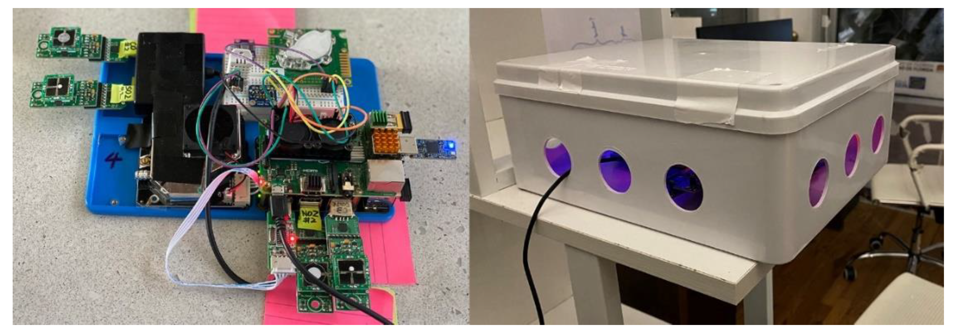
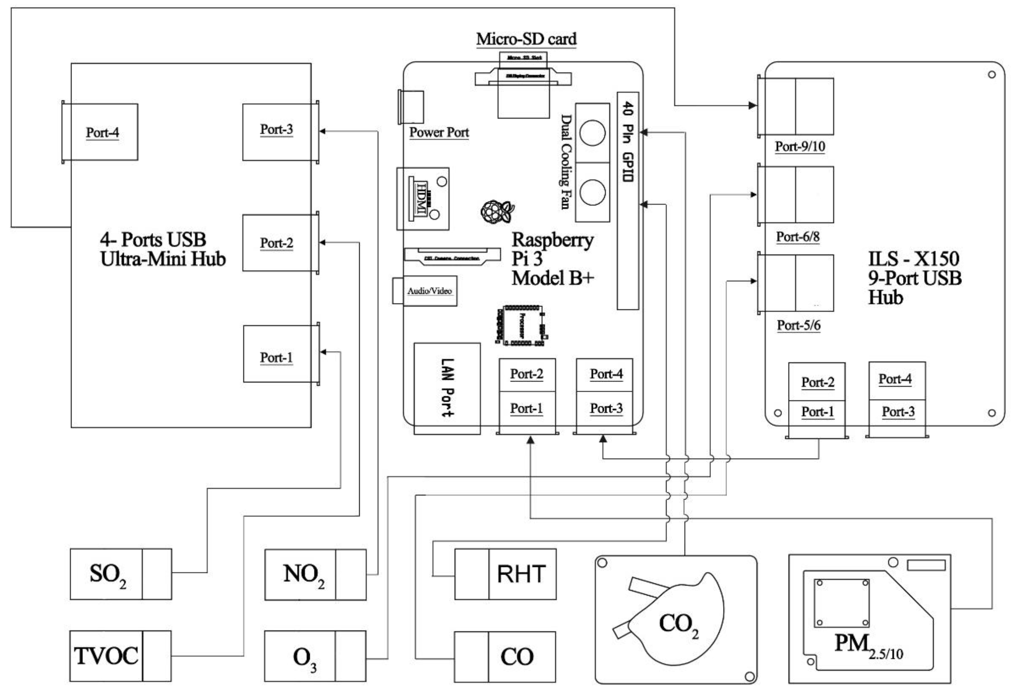
2. Low Cost Air Quality System

The custom built LCAQS monitoring system used for this project was developed on a Raspberry Pi 3B Plus module. This module is a low-power, compact, easily configurable SBC which is powered by an ARM Cortex-A53 processor [43]. The Raspberry Pi module encompasses features such as a Micro SD port for external storage access, Bluetooth, wireless LAN, USB ports, and GPIO pins for external communication. A nine-port expansion board was integrated into the Raspberry Pi module. A Wi-Fi USB adapter was connected to the Gigabit Ethernet port to establish access to the internet. In order to dissipate excess operational heat, a dual fan and heat sink module was attached to the Raspberry Pi system. Figure 1 shows the custom-built LCAQS monitoring system, and Figure 2 depicts a detailed block diagram with all electrical connections. The sensors used in this study were selected from the author’s previous publication [8] accounting for repeatability, tolerance, and response time.
The DHT22 sensor is utilized to measure humidity and temperature levels. The sensor is connected to the Raspberry Pi module through a 5k pull-up resistor using I/O pins. The measuring capacity of the sensor ranges between −40 °F and 176 °F with ±0.5 °F accuracy for temperature and from 0% to 100% with ±2–5% accuracy or humidity [44]. DHT22 outputs humidity and temperature values as serial data. The SDS 011 sensor measures particulate matter between 0.3 and 10 μm in diameter using a laser scattering technique. The sensor with a built-in fan is interfaced with the Raspberry Pi module using an UART (universal asynchronous receiver-transmitter) connection. SDS 011 with a quick response time (<10 s) can measure particulate matter concentrations between 0 and 999 μg/m³ with ±15% accuracy [45]. PM2.5 and PM10 are outputted in the form of PWM (Pulse Width Modulation) output.
The SPEC-DGS-NO2 968-043 is a low-power IoT integrated gas sensor used to measure NO2 levels. The sensor with a circuit voltage of 3 volts is interfaced with the Raspberry Pi module using an UART connection. DGS-NO2-968-043, with a response time of fewer than 30 s and repeatability less than ±3% of the reading, can measure NO2 concentrations between 0 and 5 ppm [46]. The SPEC-DGS-SO2-968-038 is a high-performance IoT integrated gas sensor used to measure SO2 levels. The sensor with a circuit voltage of 3 volts is interfaced with the Raspberry Pi module using an UART connection. DGS-SO2 968-038 with a response time of less than 30 s and repeatability less than ±3% of the reading can measure SO2 concentrations between 0 and 20 ppm [47]. The Senseair K30 is an OEM (original equipment manufacturer) module which is customized as a sensor platform to measure CO2 gas. The sensor uses the NDIR (non-dispersive infrared) technique to detect CO2 levels in a region. The module is interfaced with Raspberry Pi using an UART connection. SenseAir K30, with a quick response time of 20 s, can measure CO2 concentrations between 0 and 5000 ppm with accuracy of ±3% of the reading [48]. The SPEC-DGS-CO 968-034 is a lightweight IoT integrated gas sensor used to measure CO levels. The sensor with a circuit voltage of 3.3 volts is interfaced with the Raspberry Pi module using an UART connection. DGS-CO-968-034 with a typical response time of 15 s and repeatability less than ±3% of the reading (or 2 ppm, whichever is greater) can measure CO concentrations between 0 and 1000 ppm [49]. The SPEC-DGS-O3-968-042 is an ultra-low power consumption IoT integrated gas sensor used to measure O3 levels. The sensor with a circuit voltage of 3.3 volts is interfaced with the Raspberry Pi module using an UART connection. DGS-O3-968-042 with a response time of less than 30 s and repeatability less than ±3% of the reading can measure O3 concentrations between 0 and 5 ppm [50]. The uThing::VOC™ is an open access USB module which utilizes the Bosch BME680 air quality sensor to detect VOCs (volatile organic compounds) [51]. The BME680 sensor mainly detects compounds such as ethane, ethanol, acetone, and isoprene with an accuracy of 5%. The module is integrated with Raspberry Pi using a simple USB connection, and the VCP (virtual communication port) interface is utilized to export data as a CSV (comma-separated values) file. The sensor with a response time of less than one second outputs an IAQ index between 0 and 500 based on EPA guidelines, which corresponds to the VOC concentrations [51]. The specifications and the market price of this LCAQS are shown in Table 1. Based on the official datasheets and specifications, the sensor modules chosen for this LCAQS are pre-calibrated in the factory with FRM/FEM equipment and therefore required no end-user calibration.

3. Measurements Using LCAQS

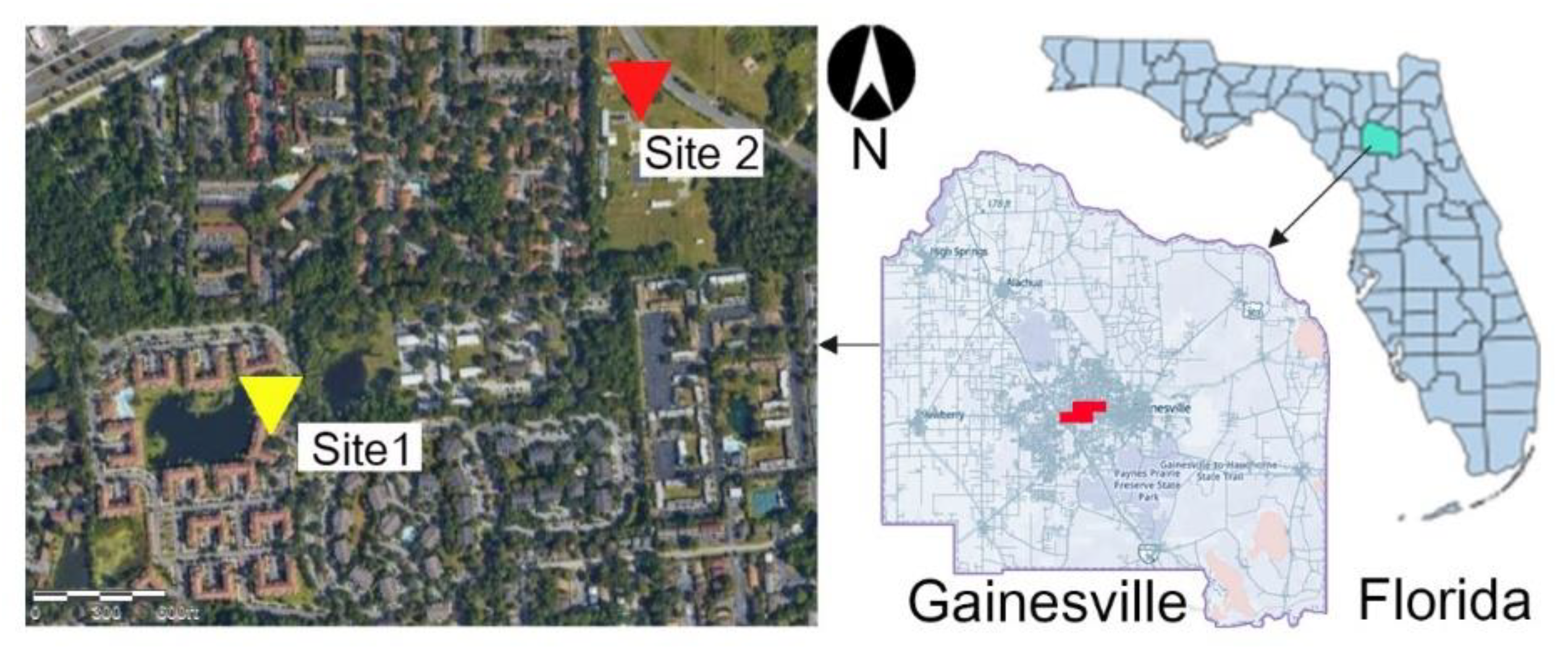
3.1. Site-Description

The two sites (Figure 3) chosen for this experiment were a university lab building and the living room of a two-bedroom residential apartment unit, both located in the city of Gainesville, Florida, United States. Gainesville is an inland city located in Alachua County of Central Florida, which experiences a humid subtropical climate all year-round. The lab building is an educational office space with a plywood floored area of 321 sq.ft situated at a distance of 245 ft from the nearest major road. A 1.5-ton ducted split-type indoor air conditioning unit (Mitsubishi PEA-A18AA) provides centralized cooling for the room while the air handling unit maintains a constant airflow rate of 235 CFM [52]. This HVAC unit is coupled with a washable MERV-8 air filter with a PM2.5 removal efficiency of 20–35% [53]. The mechanically ventilated space has three operable windows, which are closed at all times. Due to the COVID pandemic, the occupancy capacity is limited to a maximum of three people at a given time. The living room is part of a standard two-bedroom residential unit. The unit is located on the second floor of a three-story building with a carpet floor area of 421 sq.ft. A 4-ton centralized air conditioning unit (GOODMAN GSX13048-AWUF24051BA) provides cooling, and the air handling unit maintains a constant airflow rate of 835 CFM [54]. This HVAC unit is coupled with a MERV-8 air filter with a PM2.5 removal efficiency of 20–35% [53]. The mechanically ventilated space has two operable windows, which are closed at all times. The occupancy capacity is limited to a maximum of three people throughout the year. The distance between the two experimental sites is 2272.30 ft. The air conditioning units at both sites continuously function throughout the year. The experimental sites were chosen to study variations in air quality among two similar spaces with different functional purposes.

3.2. Measuring and Sampling Methods
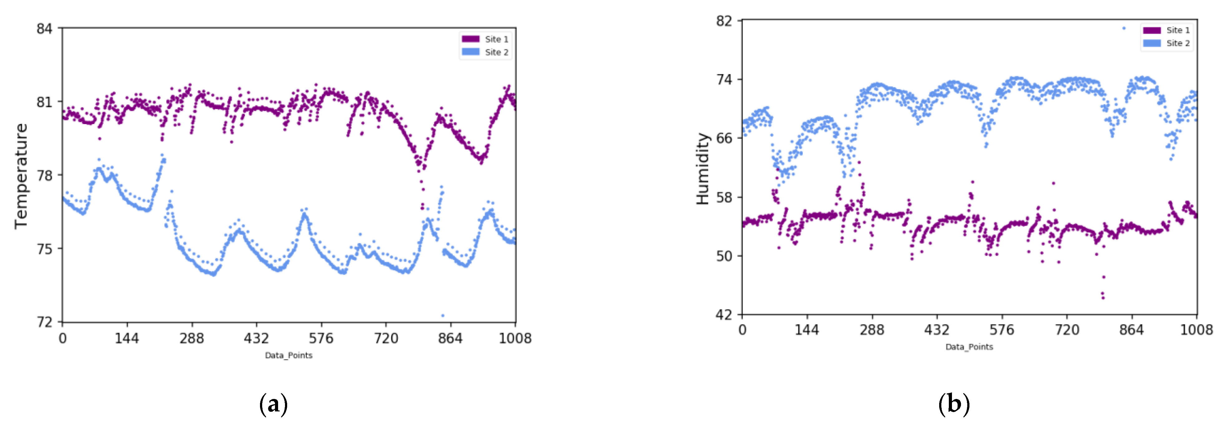
Two distinct time periods spanning seven days were selected to conduct the experiments at the two respective locations. For the residential unit, data were collected between 8 September 2020 and 14 September 2020 while for the educational building, air quality was monitored from 17 September 2020 to 23 September 2020. In total, the 10 air quality parameters measured were relative humidity, temperature, PM2.5, PM10, NO2, SO2, CO2, CO, O3, and TVOC. In order to structure the monitoring process to limit measurement uncertainties, the standardized EPA monitoring protocol for indoor air quality was implemented [10]. The ASHRAE 62.1-2019 standard was utilized for analyzing each air pollutant concentration [55]. In both monitoring locations, the LCAQS system was placed 3.7 feet above floor level, 1.5 feet away from a wall, and at least a 4.8 feet distance from any corner. Each of the two LCAQS systems deployed at both locations collects 24-h continuous data in intervals of 10-min for all of the pollutants mentioned [10,27,56,57].

3.3. Data Analysis

The data measured by the LCQAS systems are extracted and subjected to statistical analyses to understand the effects of indoor pollutant concentrations on air quality. Python (version 3.6.12) language was used to conduct descriptive analysis to determine statistical parameters such as mean, standard deviation, and variance. A quantile-quantile (Q-Q) plot was produced in Python to study the distribution pattern of the data set. Correlation studies were carried out in RStudio software (version 1.3.1093) to study the inter-dependency and influence of one pollutant on another. The monotonic relationship between pollutants was determined using Spearman rank-order correlation. The Spearman correlation coefficient ranging between −1 and 1 was utilized to establish a degree of correlation within pollutants, while a minimum sensitivity of <0.05 was considered significant [58,59,60].

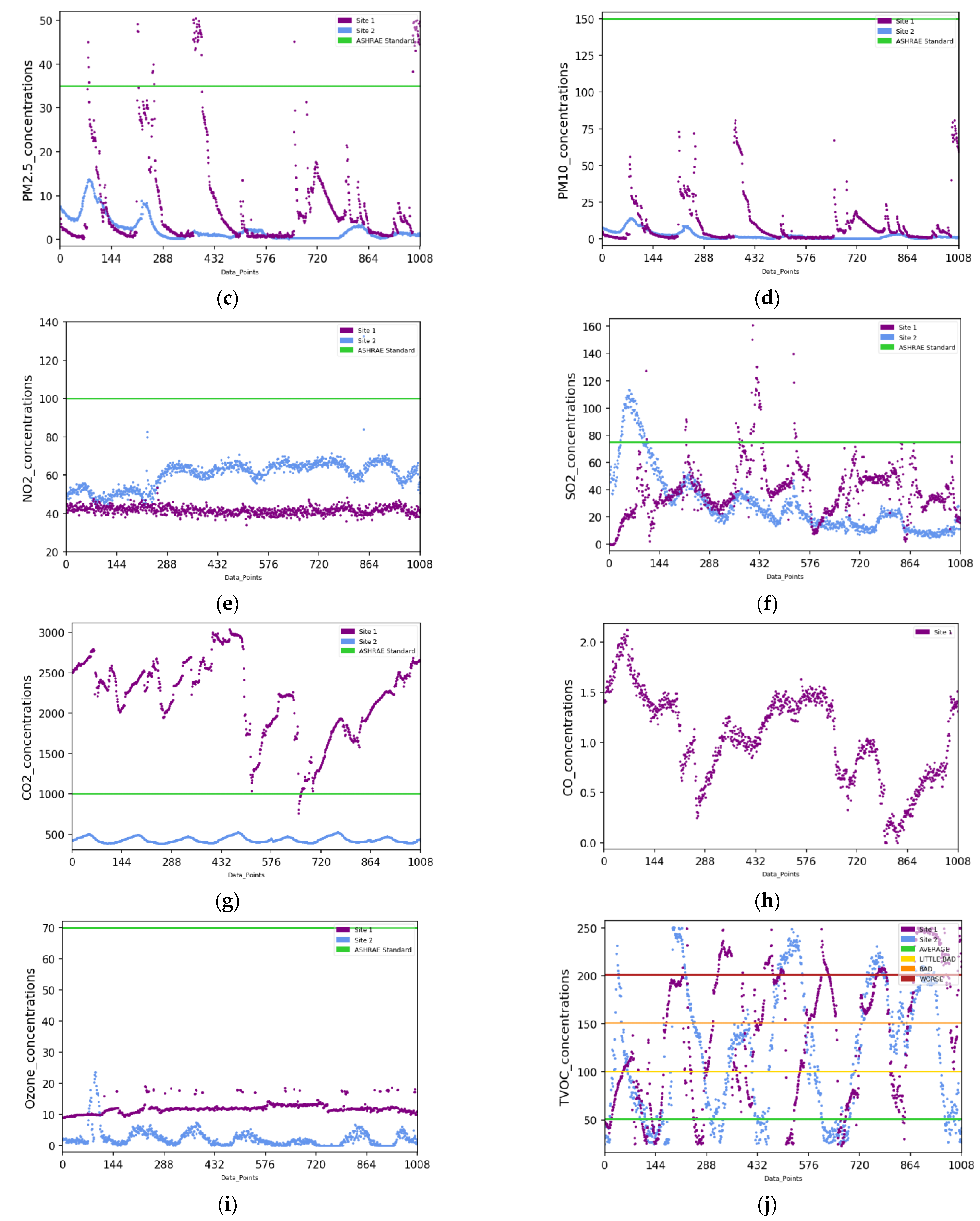
4. Results and Discussion

The custom-built LCAQS system was deployed in two locations, namely: site 1 (a living room within a residential apartment unit) and site 2 (an educational office space). The system successfully gathered concurrent data from all of the individual sensor modules without hindrance at both respective locations. The values of monitored pollutants were extracted from the LCAQS system and transferred to an external computer without data attenuation.
Table 2 shows the monitored average environmental parameters along with its standard deviation, minimum, and maximum levels. Site 1 has a mean temperature and humidity of 80.5 ℉ and 45.5%, while site 2 has a relatively lower mean temperature of 75.5 ℉ and a higher mean humidity of 70.4%. The PM2.5 and PM10 concentrations for site one range between 0.20 and 50.5 µg/m3 and 0.20 and 80.9 µg/m3 while recording mean values of 8.53 and 10.2 µg/m3, respectively. The average PM2.5 and PM10 concentrations for site 2 are comparatively lower at 2.33 and 2.43 µg/m3. The mean NO2 concentration for site 2 at 60.3 ppb is relatively higher than that of site 1 at 41.8 ppb, and the corresponding standard deviation follows a similar trend at 2.02 for site 1 and 6.94 for site 2. Site 1 has a mean SO2 value of 39.9 ppb, while site 2 has a relatively lower value of 29.6 ppb. The minimum CO2 concentration of 761 ppm recorded at site 1 is greater than the maximum value of 522 ppm registered at site 2. Similarly, the mean concentration of 2195 ppm at site 1 is significantly higher than the mean value of 432 ppm at site 2. Since the collected CO data for site 2 was mostly negligible in value, it was deemed as statistically insignificant for this study. For site 1, the average CO concentration is 1.05 ppb, and the maximum value recorded is 2.12 ppb. The mean ozone level for site 1 at 12.1 ppb is over five times greater than the mean concentration of 2.37 ppb registered at site 2. The recorded TVOC values were measured against the IAQ index scale ranging from 0 to 500. Site 1 has an average TVOC level of 139.2, and site 2 has a value of 121 while the maximum value for both sites is 250.
The PM2.5 and PM10 concentrations follow a similar pattern for both site 1 and site 2 as plotted in Figure 4c,d. For the first three days, distinctive peaks varying in amplitudes are visible around midday for the particulate matter at Sites 1 and 2. The crests with higher values at site 1 can be attributed to scheduled cooking activities when compared to relatively shorter peaks at site 2, which may be due to increased human activity during lunch breaks and increased nearby vehicular traffic. These peaks can be compared against the ASHRAE 62.1-2019 standard for the particulate matter, which is 35 µg/m3 (24 h) for PM2.5 and 150 µg/m3 (24 h) for PM10. Some of the data points for PM2.5 exceed the ASHRAE 62.1-2019 [55] standard during mid-day, while PM10 exclusively lies below the standard. On the latter half of the fifth day, a spike is detected starting in the late evening. This anomaly might be due to an organized house event containing three people, subsequently leading to increased house activity. This event can also be viewed in terms of increased pollutant concentrations simultaneously across PM10, CO2, SO2, and TVOC. From Figure 4e, the NO2 concentrations for site 1 show a significantly stable pattern across the seven-day monitoring period. The potential reason for this trend could be the lack of NO2 emitting sources. The recurring smooth crests for site 2 can be attributed to a gradual increase in traffic-related pollution over the course of the day peaking at midday. The ASHRAE 62.1-2019 standard for NO2 is 100 ppb (1 h), and at both sites the NO2 levels recorded are below this standard. The SO2 concentrations follow a relatively similar trend for both site 1 and site 2, as plotted in Figure 4f. The ASHRAE 62.1-2019 standard for SO2 is 75 ppb (1 h), and at both sites, some data points recorded oscillate above this standard. The CO2 concentrations for site 2 show a significantly low value exhibiting a stable pattern across the span of seven-days, as viewed in Figure 4g. The potential reason for this trend could be because of increased sedentary human behavior within the office space. The ASHRAE 62.1-2019 standard for CO2 is 1000 ppm (24 h), and at site 2, the CO2 levels registered are below this standard. Most of the data points are above the standard for Site 1, which might be due to factors such as CO2 exhalation from increased people count, cooking, and emissions from household cleaning products. The CO concentrations detected in site 1 portray a relatively low value when compared to the ASHRAE 62.1-2019 standard for CO, which is 9 ppm (8 h). Figure 4i shows O3 concentrations where site 1 displays a significantly stable pattern across the entirety of the study period. The possible reason for this trend could be a lack of nearby vehicular-emissions, which is a primary source of ground-level O3. The repeating low-amplitude smooth peaks for site 2 can be attributed to locational proximity to traffic-related pollution over the course of the day. Both sites recorded O3 levels below the ASHRAE 62.1-2019 standard of 70 ppb (8 h). The measured TVOC data is mapped onto the IAQ index scale, which classifies air quality on a scale of 0 to 500 as: good (0–50), average (51–100), little bad (101–150), bad (151–200), worse (201–300), and very bad (301–500) [51,61]. As depicted in Figure 4j, the data oscillates, leaving only a few observation points below the acceptable good standard, and some even exceed the worse standard line. Both sites display TVOC concentrations that peak at varying amplitudes throughout the study period around midday. The only exception is day five at site 2 where the decline in TVOC levels can be attributed to the absence of occupants. This decline in concentration is also simultaneously seen in PM2.5, PM10, and O3.
Quantile-Quantile (Q-Q) plots [62,63] are used to characterize the distribution of measured values at Site 1 and 2. Based on the spread of observational points, the type of distribution can be determined by visually characterizing the data sets with respect to the identity line. If most of the measured points are concentrated along the identity line sharing a similar slope, then the data are normally distributed while a deviation above (high-bias) or below (low-bias) the identity line indicates a skewed distribution. From Figure 5, the PM2.5 and PM10 data are normally distributed with limited deviation from the identity line for low to medium concentrations and exhibit a low-bias towards higher concentrations. For NO2, the observational points are concentrated towards the low and medium spectrum of the data range, while a few points exist away from the distribution for higher concentrations. The slope of TVOC distribution is the most identical to that of the identity line, thereby displaying a high degree of normal distribution while indicating a high closeness in trend between Site 1 and 2. Pollutants such as SO2 and CO2 depict a substantial positive and negative deviation respectively across medium and higher concentrations resulting in a skewed distribution. From lower to medium pollutant levels, O3 has a relatively normal distribution. At higher concentrations, the plot shows a greater positive deviation from the identity line.
The Spearman rank-order analysis was used to estimate the strength of the correlation between two measured parameters by assigning a ranked value (R) between −1 and 1 [58,59,64]. According to Figure 6, site 2 exhibits a relatively stronger correlation among environmental parameters compared to site 1. Site 1 shows that SO2 has a strong correlation with PM2.5 (R = 0.9) and PM10 (R = 0.83). This trend can also be found at site 2 among PM2.5 (R = 0.92) and PM10 (R = 0.9). This can be attributed to cooking activities in site 1 and vehicular pollution at site 2, which both contribute to increasing levels of SO2, PM2.5, and PM10 [17,65,66]. Both sites 1 and 2 have the same degree of negative correlation between O3 and humidity (R = −0.78). The higher O3 concentrations can be due to increased solar irradiation corresponding to low relative humidity-high temperature surroundings. The temperature values recorded at site 2 shows strong correlations with O3 (R = 0.78), SO2 (R = 0.8), PM2.5 (R = 0.88), and PM10 (R = 0.9). An increase in temperature results in dry air, which might aggregate higher concentrations of PM2.5, and PM10 in a city environment. The relationship between temperature and O3, SO2, and PM2.5 is similar with the results observed by Mahmoud while exhibiting stronger degrees of correlation [67]. O3 has a strong correlation with PM2.5 (R = 0.8) and PM10 (R = 0.82) at site 2. There is a moderate correlation between temperature and TVOC (R = −0.65) at site 1. Similarly, temperature and TVOC share a moderate correlation (R = −0.72) at site 2. The similar negative correlation between TVOC and temperature within an office space was observed by Otolorin et al. [68]. Site 1 displays a moderate correlation between humidity and SO2 (R= −0.62), while site 2 exhibits a comparatively stronger correlation (R= −0.8). SO2 has the tendency to react with water vapor present in building walls and furniture, which may lead to decreasing concentrations of SO2 as the humidity increases [12,13,20]. There is a moderate correlation (R = 0.58) between humidity and CO2 at site 1 and a strong correlation (R = 0.78) at site 2. Site 1 has a low correlation between NO2 and CO2 (R = 0.47), while site 2 exhibits a relatively stronger correlation (R = 0.77). This might be due to human activities in site 1 and traffic-related pollution at site 2. This correlation between NO2 and CO2 is consistent with the study performed by S.H. Hwang [69]. There is a strong correlation at site 2 between humidity and NO2 (R = 0.98) and a relatively weaker correlation at site 1 (R = 0.45). At site 1 there is a moderate correlation between CO2 and O3 (R = −0.5) while site 2 displays a stronger correlation (R = −0.9) and this may be because of insufficient ventilation [6,15,70]. Site 2 registered a moderate correlation between humidity and TVOC (R = 0.72). The NO2 values of site 2 show a moderate correlation with TVOC (R = 0.73) and have a relatively stronger correlation with humidity (R = 0.98). This may be attributed to the presence of high-emitting building materials and fuel-burning household appliances at the residential unit [17,20,66].

5. Conclusions

In this paper, a comprehensive environmental monitoring system is presented which detects most of the critical indoor air pollutants. Multiple independent sensors were selected accounting for repeatability, tolerance, and response time. These individual sensor modules were integrated onto a Python-powered Raspberry Pi platform to form a single LCAQS system to measure, analyze, and determine indoor air quality. The multi-sensor module recorded environmental parameters such as temperature, relative humidity, PM2.5, PM10, NO2, SO2, CO2, CO, O3, and TVOC in real-time at regular 10-min intervals. The logged data was extracted from the LCAQS system and transferred to a computer using an open-source network file transfer application, PuTTY.
It was observed that both PM2.5 and PM10 concentrations were significantly higher in the residential apartment unit (site 1) than at the office space (site 2) while the former recorded maximum values of 50.5 and 80.9µg/m3, respectively. Sites 1 and 2 registered to mean NO2 levels of 41.8 and 60.3 ppb, respectively, while site 2 displayed a wider range of observed data between 43.8 and 132 ppb. The highest difference in concentration levels was observed with CO2, as site 1 (2195 ppm) exhibited CO2 values that were more than five times greater than those of site 2 (432 ppm). Although both sites 1 and 2 displayed comparatively close levels of SO2 at 39.9 and 29.6 ppb, respectively, the maximum concentration was observed at site 1 at 161 ppb. The mean O3 concentration recorded at site 1 at 12.1 ppb was significantly higher compared to site 2 at 2.37 ppb. Both sites registered the same maximum TVOC value of 250, while site 1 displayed a slightly higher average value of 139.2 to that of site 2 at 121.
Spearman rank-order analysis indicates that PM2.5, and PM10 has a strong correlation with SO2 at both site 1 and site 2. The potential reason for this can be cooking activities in site 1 and vehicular pollution at site 2, which both contribute to increasing levels of PM2.5, PM10, and SO2. O3 concentrations at site 2 exhibit a strong correlation with PM2.5 and PM10. NO2 and CO2 show a relatively stronger correlation at site 1 when compared to site 2, and this might be due to human activities in site 1 and combustion-related pollution at site 2. Similarly, NO2 and TVOC display moderate correlation at site 2. There is a moderate correlation between CO2 and O3 at site 1, while site 2 shows a relatively stronger correlation, and this might be due to insufficient ventilation. The possible effect of an increased number of human occupants on environmental pollutants can be witnessed at site 2, which displays strong temperature and humidity correlation with O3, SO2, PM2.5, and PM10 when compared to site 1.
The constituent sensors of the custom-built LCAQS system utilized in this study rely on factory calibration. It is a challenge to individually calibrate all the sensors owing to limited availability and high cost of calibration equipment in the market for certain pollutants. Owing to the latter, limited efforts have been taken to validate the obtained results with a reference monitor. For future studies, sensor parameters such as such as precision, short and long term drift, and power supply effect can be tested by devising operational rigidity experiments on the sensors to ensure the accuracy of obtained results. Furthermore, the correlation values derived in this paper may need to be examined further to arrive at a conclusive inference. This can be achieved by monitoring air quality for longer periods across different locational settings accounting for varied surrounding-related influences. Moreover, Principal Component Analysis (PCA) can be undertaken to reduce the multicollinearity of measured parameters. Also, mixed-effect linear regression models are suggested to better study the association between indoor air pollutants and building characteristics.

Supplementary Materials

The supplementary materials are available online at https://www.mdpi.com/2071-1050/13/1/370/s1.

Author Contributions

H.Z.; Sensor Development: H.Z.; Data collection and analysis: H.Z. and V.G.; Writing—Original draft: H.Z. and V.G.; writing—Review and editing: R.S.; supervision: R.S. All authors have read and agreed to the published version of the manuscript.

Funding

This research received no external funding.

Informed Consent Statement

Not applicable.

Data Availability Statement

The data presented in this study are available in supplementary material.

Conflicts of Interest

The authors declare no conflict of interest.

References

  1. ALA. The State of the Air 2020; American Lung Association: Chicago, IL, USA, 2020; pp. 1–57. [Google Scholar]
  2. Pitarma, R.; Marques, G.; Ferreira, B.R. Monitoring Indoor Air Quality for Enhanced Occupational Health. J. Med. Syst. 2017, 41, 1–8. [Google Scholar] [CrossRef] [PubMed]
  3. Ritchie, H.; Roser, M. Indoor Air Pollution. Our World Data 2020. Available online: https://ourworldindata.org/indoor-air-pollution (accessed on 3 November 2020).
  4. Andersson, K. TVOC and health in non-industrial indoor environments report from a Nordic scientific consensus meeting at Langholmen in Stockholm, 1996. Indoor Air 1997, 7, 78–91. [Google Scholar] [CrossRef]
  5. Saeki, Y.; Kadonosono, K.; Uchio, E. Clinical and allergological analysis of ocular manifestations of sick building syndrome. Clin. Ophthalmol. 2017, 11, 517–522. [Google Scholar] [CrossRef] [PubMed] [Green Version]
  6. Ahmed Abdul-Wahab, S.A.; En, S.C.F.; Elkamel, A.; Ahmadi, L.; Yetilmezsoy, K. A review of standards and guidelines set by international bodies for the parameters of indoor air quality. Atmos. Pollut. Res. 2015, 6, 751–767. [Google Scholar] [CrossRef]
  7. Menzies, D.; Bourbeau, J. Building-Related Illnesses. N. Engl. J. Med. 1997, 337, 1524–1531. [Google Scholar] [CrossRef] [PubMed]
  8. Zhang, H.; Srinivasan, R. A systematic review of air quality sensors, guidelines, and measurement studies for indoor air quality management. Sustainability 2020, 12, 9045. [Google Scholar] [CrossRef]
  9. Wagner, J.G.; Kamal, A.S.; Morishita, M.; Dvonch, J.T.; Harkema, J.R.; Rohr, A.C. PM2.5-Induced cardiovascular dysregulation in rats is associated with elemental carbon and temperature-resolved carbon subfractions. Part. Fibre Toxicol. 2014, 11, 25. [Google Scholar] [CrossRef] [Green Version]
  10. EPA. A Standardized EPA Protocol for Characterizing Indoor Air Quality in Large Office Buildings; EPA: Washington, DC, USA, 2016.
  11. Branco, P.T.B.S.; Nunes, R.A.O.; Alvim-Ferraz, M.C.M.; Martins, F.G.; Sousa, S.I.V. Children’s exposure to indoor air in urban nurseries—Part II: Gaseous pollutants’ assessment. Environ. Res. 2015, 142, 662–670. [Google Scholar] [CrossRef] [Green Version]
  12. NAAQS. Primary National Ambient Air Quality Standard (NAAQS) for Sulfur Dioxide. Available online: https://www.epa.gov/so2-pollution/primary-national-ambient-air-quality-standard-naaqs-sulfur-dioxide (accessed on 26 July 2019).
  13. Spengler, J.D.; Ferris, B.G.; Dockery, D.W.; Speizer, F.E. Sulfur Dioxide and Nitrogen Dioxide Levels Inside and Outside Homes and the Implications on Health Effects Research. Environ. Sci. Technol. 1979, 13, 1276–1280. [Google Scholar] [CrossRef]
  14. Johnson, D.L.; Lynch, R.A.; Floyd, E.L.; Wang, J.; Bartels, J.N. Indoor air quality in classrooms: Environmental measures and effective ventilation rate modeling in urban elementary schools. Build. Environ. 2018, 136, 185–197. [Google Scholar] [CrossRef]
  15. Madureira, J.; Paciência, I.; Rufo, J.; Severo, M.; Ramos, E.; Barros, H.; de Oliveira Fernandez, E. Source apportionment of CO2, PM10 and VOCs levels and health risk assessment in naturally ventilated primary schools in Porto, Portugal. Build. Environ. 2016, 96, 198–205. [Google Scholar] [CrossRef] [Green Version]
  16. Seltzer, J.M. Building-related illnesses. J. Allergy Clin. Immunol. 1994, 94, 351–361. [Google Scholar] [CrossRef] [PubMed]
  17. Civan, M.Y.; Elbir, T.; Seyfioglu, R.; Kuntasal, Ö.O.; Bayram, A.; Doğan, G.; Yurdakul, S.; Andiç, Ö.; Müezzinoğlu, A.; Sofuoglu, S.C.; et al. Spatial and temporal variations in atmospheric VOCs, NO2, SO2, and O3 concentrations at a heavily industrialized region in Western Turkey, and assessment of the carcinogenic risk levels of benzene. Atmos. Environ. 2015, 103, 102–113. [Google Scholar] [CrossRef] [Green Version]
  18. EPA. Building Air Quality—A Guide for Building Owners and Facility Managers; EPA-402-F-91-102; EPA: Washington, DC, USA, 1991; pp. 1–228.
  19. WHO. WHO Guidelines for Indoor Air Quality: Selected Pollutants; WHO: Copenhagen, Denmark, 2010; Volume 35. [Google Scholar]
  20. Gvozdić, V.; Kovač-Andrić, E.; Brana, J. Influence of Meteorological Factors NO2, SO2, CO and PM10 on the Concentration of O3 in the Urban Atmosphere of Eastern Croatia. Environ. Model. Assess. 2011, 16, 491–501. [Google Scholar] [CrossRef]
  21. Yang, J.; Seo, J.H.; Jeong, N.N.; Sohn, J.R. Effects of Legal Regulation on Indoor Air Quality in Facilities for Sensitive Populations—A Field Study in Seoul, Korea. Environ. Manag. 2019, 64, 344–352. [Google Scholar] [CrossRef]
  22. Fishbain, B.; Lerner, U.; Castell, N.; Cole-Hunter, T.; Popoola, O.; Broday, D.M.; Martinez Iniquez, T.; Nieuwenhuijsen, M.; Jovasevic-Stojanovic, M.; Topalovic, D.; et al. An evaluation tool kit of air quality micro-sensing units. Sci. Total Environ. 2017, 575, 639–648. [Google Scholar] [CrossRef]
  23. Munir, S.; Mayfield, M.; Coca, D.; Jubb, S.A.; Osammor, O. Analysing the performance of low-cost air quality sensors, their drivers, relative benefits and calibration in cities—A case study in Sheffield. Environ. Monit. Assess. 2019, 191. [Google Scholar] [CrossRef] [Green Version]
  24. Clements, A.L.; Griswold, W.G.; Abhijit, R.S.; Johnston, J.E.; Herting, M.M.; Thorson, J.; Collier-Oxandale, A.; Hannigan, M. Low-Cost air quality monitoring tools: From research to practice (A workshop summary). Sensors 2017, 17, 2478. [Google Scholar] [CrossRef] [Green Version]
  25. Williams, R.; Kilaru, V.J.; Snyder, E.G.; Kaufman, A.; Dye, T.; Rutter, A.; Russel, A.; Hafner, H. Air Sensor Guidebook; National Exposure Research Laboratory: Research Triangle Park, NC, USA, 2014. [CrossRef]
  26. Williams, R. Tools and Resources Webinar: Low Cost Air Quality Sensors; EPA: Washington, DC, USA, 2019.
  27. Morawska, L.; Thai, P.K.; Liu, X.; Asumadu-Sakyi, A.; Ayoko, G.; Bartonova, A.; Bedini, A.; Chai, F.; Christensen, B.; Dunbabin, M.; et al. Applications of low-cost sensing technologies for air quality monitoring and exposure assessment: How far have they gone? Environ. Int. 2018, 116, 286–299. [Google Scholar] [CrossRef]
  28. Polidori, A.; Papapostolou, V.; Zhang, H. Laboratory Evaluation of Low-Cost Air Quality Sensors; South Coast AQMD: Diamond Bar, CA, USA, 2016.
  29. AQ-SPEC. Laboratory Evaluation Air Quality Egg 2018 Model; South Coast AQMD: Diamond Bar, CA, USA, 2018.
  30. Giusto, E.; Gandino, F.; Greco, M.L.; Grosso, M.; Montrucchio, B.; Rinaudo, S. An investigation on pervasive technologies for IoT-based thermal monitoring. Sensors 2019, 19, 663. [Google Scholar] [CrossRef] [Green Version]
  31. Thompson, J.E. Crowd-Sourced air quality studies: A review of the literature & portable sensors. Trends Environ. Anal. Chem. 2016, 11, 23–34. [Google Scholar] [CrossRef]
  32. Abraham, S.; Li, X. A cost-effective wireless sensor network system for indoor air quality monitoring applications. Procedia Comput. Sci. 2014, 34, 165–171. [Google Scholar] [CrossRef] [Green Version]
  33. Zhou, M.; Abdulghani, A.M.; Imran, M.A.; Abbasi, Q.H. Internet of Things (IoT) Enabled Smart Indoor Air Quality Monitoring System. ACM Int. Conf. Proc. Ser. 2020, 89–93. [Google Scholar] [CrossRef]
  34. Mohd Pu’ad, M.F.; Gunawan, T.S.; Kartiwi, M.; Janin, Z. Performance evaluation of portable air quality measurement system using raspberry Pi for remote monitoring. Indones. J. Electr. Eng. Comput. Sci. 2019, 17, 564–574. [Google Scholar] [CrossRef] [Green Version]
  35. Kumar, S.; Jasuja, A. Air quality monitoring system based on IoT using Raspberry Pi. In Proceedings of the 2017 IEEE International Conference on Computing, Communication and Automation (ICCCA), Greater Noida, India, 5–6 May 2017; pp. 1341–1346. [Google Scholar] [CrossRef]
  36. Saha, A.K.; Sircar, S.; Chatterjee, P.; Dutta, S.; Mitra, A.; Chatterjee, A.; Chattopadhyay, S.P.; Saha, H.N. A raspberry Pi controlled cloud based air and sound pollution monitoring system with temperature and humidity sensing. In Proceedings of the 2018 IEEE 8th Annual Computing and Communication Workshop and Conference (CCWC), Las Vegas, NV, USA, 8–10 January 2018; pp. 607–611. [Google Scholar] [CrossRef]
  37. Kiruthika, R.; Umamakeswari, A. Low cost pollution control and air quality monitoring system using Raspberry Pi for Internet of Things. In Proceedings of the 2017 International Conference on Energy, Communication, Data Analytics and Soft Compututing (ICECDS), Chennai, India, 1–2 August 2017; pp. 2319–2326. [Google Scholar] [CrossRef]
  38. Alkandari, A.A.; Moein, S. Implementation of monitoring system for air quality using raspberry Pi: Experimental study. Indones. J. Electr. Eng. Comput. Sci. 2018, 10, 43–49. [Google Scholar] [CrossRef]
  39. Ali, A.S.; Zanzinger, Z.; Debose, D.; Stephens, B. Open Source Building Science Sensors (OSBSS): A low-cost Arduino-based platform for long-term indoor environmental data collection. Build. Environ. 2016, 100, 114–126. [Google Scholar] [CrossRef] [Green Version]
  40. Parkinson, T.; Parkinson, A.; de Dear, R. Continuous IEQ monitoring system: Performance specifications and thermal comfort classification. Build. Environ. 2019, 149, 241–252. [Google Scholar] [CrossRef] [Green Version]
  41. Mejía, J.F.; Choy, S.L.; Mengersen, K.; Morawska, L. Methodology for assessing exposure and impacts of air pollutants in school children: Data collection, analysis and health effects—A literature review. Atmos. Environ. 2011, 45, 813–823. [Google Scholar] [CrossRef]
  42. WHO. Risk of Bias Assesssment Instrument for Systematic; WHO Regional Office for Europe: Copenhagen, Denmark, 2020. [Google Scholar]
  43. Raspberry, P. Raspberry Pi 3 Model B+ Datasheet; Raspberry Pi Ltd.: Milton, UK, 2016; p. 5. [Google Scholar]
  44. DHT22. Digital-Output Relative Humidity & Temperature Sensor/Module AM2303, DHT22, Datasheet; Aosong Electron Co, Ltd.: Guangzhou, China, 2015; Available online: https://www.electroschematics.com/wp-content/uploads/2015/02/DHT22-datasheet.pdf (accessed on 20 June 2020).
  45. Nova Fitness Co., Ltd. PM2.5 L. Laser PM2.5 Sensor. Available online: https://cdn-reichelt.de/documents/datenblatt/X200/SDS011-DATASHEET.pdf (accessed on 31 July 2019).
  46. SPEC Sensors. DGS-NO2 986-042, Digital Gas Sensor—Ozone. Available online: https://media.digikey.com/pdf/DataSheets/SPECSensorsPDFs/968-043_9-6-17.pdf (accessed on 25 July 2019).
  47. SPEC Sensors. DGS-SO2 986-042, Digital Gas Sensor—Ozone. Available online: https://www.spec-sensors.com/wp-content/uploads/2017/01/DGS-SO2-968-038.pdf (accessed on 25 July 2019).
  48. CO2Meter. K-30.K-30. Available online: https://img.ozdisan.com/ETicaret_Dosya/456729_1584920.PDF (accessed on 30 July 2019).
  49. Digi-Key Electronics. 968-034 D-C, Digital Gas Sensor—Carbon Monoxide. Available online: https://www.digikey.com/en/products/detail/spec-sensors-llc/968-034/6676880 (accessed on 26 July 2019).
  50. SPEC Sensors. DGS-O3, Digital Gas Sensor—Ozone. Available online: https://www.spec-sensors.com/wp-content/uploads/2017/01/DGS-O3-968-042_9-6-17.pdf (accessed on 25 July 2019).
  51. Ohmetch.io. UTHING::VOCTM™ Air-Quality USB Sensor Dongle. Available online: https://ohmtech.io/products/uthingvoc/#specifications (accessed on 10 June 2019).
  52. Mitsubishi Electric. TECHNICAL & SERVICE MANUAL. PEA-A18AA. PEA-A18AA. Available online: https://www.mitsubishitechinfo.ca/sites/default/files/PEA-A12-18AA4_Service_0.pdf (accessed on 28 June 2020).
  53. EPA. What is a MERV rating? Indoor Air Quality (IAQ). Available online: https://www.epa.gov/indoor-air-quality-iaq/what-merv-rating-1 (accessed on 5 June 2020).
  54. Goodman Air Conditioning and Health. GOODMAN GSX130481 4-tons 2 Ton Central Air Conditioner Air Handler Unit (Model AWUF24051BA). Available online: https://www.goodmanmfg.com/products/air-conditioners/13-seer-gsx13 (accessed on 8 June 2020).
  55. ANSI/ASHRAE. ANSI/ASHRAE Standard 62.1-2019, Ventilation for Acceptable Indoor Air Quality; American Society of Heating, Refrigerating and Air-Conditioning Engineers: Atlanta, GA, USA, 2019. [Google Scholar]
  56. WHO. Methods for Monitoring Indoor Air Quality in Schools; WHO: Bonn, Germany, 2011. [Google Scholar]
  57. Meier, R.; Schindler, C.; Eeftens, M.; Aguilera, I.; Ducret-Stich, R.E.; Ineichen, A.; Davey, M.; Phuleria, H.C.; Probst-Hensch, N.; Tsai, M.-Y.; et al. Modeling indoor air pollution of outdoor origin in homes of SAPALDIA subjects in Switzerland. Environ. Int. 2015, 82, 85–91. [Google Scholar] [CrossRef]
  58. Majd, E.; McCormack, M.; Davis, M.; Curriero, F.; Berman, J.; Connolly, F.; Leaf, P.; Rule, A.; Green, T.; Clemons-Erby, D.; et al. Indoor air quality in inner-city schools and its associations with building characteristics and environmental factors. Environ. Res. 2019, 170, 83–91. [Google Scholar] [CrossRef]
  59. Raysoni, A.U.; Stock, T.H.; Sarnat, J.A.; Chavez, M.C.; Sarnat, S.E.; Montoya, T.; Holguin, F.; Li, W.-W. Evaluation of VOC concentrations in indoor and outdoor microenvironments at near-road schools. Environ. Pollut. 2017, 231, 681–693. [Google Scholar] [CrossRef] [PubMed]
  60. Sunyer, J.; Esnaola, M.; Alvarez-Pedrerol, M.; Forns, J.; Rivas, I.; López-Vicente, M.; Suades-Gonzalez, E.; Foraster, M.; Garcia-Esteban, R.; Basagana, X.; et al. Association between traffic-related air pollution in schools and cognitive development in primary school children: A prospective cohort study. PLoS Med. 2015, 12, e1001792. [Google Scholar] [CrossRef] [PubMed]
  61. Krzyzanowski, M.; Cohen, A. Update of WHO air quality guidelines. Air Qual. Atmos. Health 2008, 1, 7–13. [Google Scholar] [CrossRef] [Green Version]
  62. Zurbenko, I.G. Detecting and tracking changes in ozone air quality. Air Waste 1994, 44, 1089–1092. [Google Scholar] [CrossRef]
  63. Seangkiatiyuth, K.; Surapipith, V.; Tantrakarnapa, K.; Lothongkum, A. Application of the AERMOD modeling system for environmental impact assessment of NO2 emissions from a cement complex. J. Environ. Sci. 2011, 23, 931–940. [Google Scholar] [CrossRef]
  64. Hwang, S.H.; Roh, J.; Park, W.M. Evaluation of PM10, CO2, airborne bacteria, TVOCs, and formaldehyde in facilities for susceptible populations in South Korea. Environ. Pollut. 2018, 242, 700–708. [Google Scholar] [CrossRef]
  65. Scibor, M. Are we safe inside? Indoor air quality in relation to outdoor concentration of PM10 and PM2.5 and to characteristics of homes. Sustain. Cities Soc. 2019, 48, 101537. [Google Scholar] [CrossRef]
  66. Chock, D.P.; Winkler, S.L.; Chen, C. A study of the association between daily mortality and ambient air pollutant concentrations in Pittsburgh, Pennsylvania. J. Air Waste Manag. Assoc. 2000, 50, 1481–1500. [Google Scholar] [CrossRef] [Green Version]
  67. El-Sharkawy, M.F. Assessment of Ambient Air Quality Level at Different Areas inside Dammam University, Case Study. Met. Environ. Arid Land Agric. Sci. 2013, 142, 1–28. [Google Scholar] [CrossRef]
  68. Adebayo, O.J.; Abosede, O.O.; Sunday, F.B.; Ayooluwa, A.A.; Adetayo, A.J.; Ademola, S.J.; Alaba, A.F. Indoor air quality level of total volatile organic compounds (TVOCs) in a university offices. Int. J. Civ. Eng. Technol. 2018, 9, 2872–2882. [Google Scholar]
  69. Hwang, S.H.; Park, W.M. Indoor air concentrations of carbon dioxide (CO2), nitrogen dioxide (NO2), and ozone (O3) in multiple healthcare facilities. Environ. Geochem. Health 2020, 42, 1487–1496. [Google Scholar] [CrossRef] [PubMed]
  70. Dai, X.; Liu, J.; Zhang, X. Monte Carlo simulation to control indoor pollutants from indoor and outdoor sources for residential buildings in Tianjin, China. Build. Environ. 2019, 165, 106376. [Google Scholar] [CrossRef]
Figure 1. Custom built Low-Cost Air Quality Sensor (LCAQS) monitoring system placed inside a weather proof enclosure.
Sustainability 13 00370 g001
Figure 2. Detailed block diagram of the LCAQS monitoring system.
Sustainability 13 00370 g002
Figure 3. Geographical map of Gainesville city located in the state of Florida depicting monitoring locations site1(residential apartment unit) and site2 (educational office space).
Sustainability 13 00370 g003
Figure 4. Seven-day evaluation of indoor environmental parameters monitored at 10-minute intervals (144 observational points a day equating to 1008): (a) temperature, (b) relative humidity, (c) PM2.5, (d) PM10, (e) NO2, (f) SO2, (g) CO2, (h) CO, (i) O3, (j) TVOC.
Sustainability 13 00370 g004aSustainability 13 00370 g004b
Figure 5. Quantile-Quantile (Q-Q) plot of indoor pollutants: (a) PM2.5, (b) PM10, (c) NO2, (d) SO2, (e) CO2, (f) O3, and (g) TVOC with an identity line (y = x line which acts as reference to standardize the axis).
Sustainability 13 00370 g005
Figure 6. Spearman correlation heat map for indoor environmental parameters at two sites.
Sustainability 13 00370 g006
Table 1. Specifications of sensors used in the LCAQS system.
Measured ParameterExample ProductManufacturerMeasuring RangeAccuracy (Repeatability)Approx. Price
(USD). 2019
RHTDHT22Aosong Electronics40 °C–80 °C;
0% to 100%
±0.5 °C; ±1%$10
PM2.5/10SDS011Nova Fitness0.0–999.9 μg /m315%; ±10 μg/m3$30
NO2DGS-NO2 968-043SPEC Sensors0–10 ppm±15%$75
SO2DGS-SO2 968-038SPEC Sensors0–20 ppm±15%$75
CO2K-30CO2Meter0–5000 ppm±30%$80
CODGS-CO 968-034SPEC Sensors0–1000 ppm±15%$75
OzoneDGS-O3 968-042SPEC Sensors0–5 ppm±15%$75
TVOCuThing:VOC™Ohmetech.io0–500 IAQ index±15%$95
Table 2. Descriptive statistics of indoor environmental parameters measured at site 1 and site 2.
Site 1 Site 2
Environmental Parameters Average ± SDMinMaxMedianAverage ± SDMinMaxMedian
PM2.5 (µg/m3)8.53 ± 11.9 0.2050.53.602.33 ± 2.740.0013.81.20
PM10 (µg/m3)10.2 ± 16.10.2080.93.902.43 ± 2.840.0014.31.30
NO2 (ppb)41.8 ± 2.0234.153.541.860.3 ± 6.9443.813262.1
SO2 (ppb)39.9 ± 20.70.0116137.629.6 ± 23.04.7911422.6
CO2 (ppm)2195 ± 47976130392270432 ± 34.6384522424
CO (ppb)1.05 ± 0.450.002.121.06N/AN/AN/AN/A
Ozone (ppb)12.1 ± 1.849.1019.111.92.37 ± 2.920.0023.71.65
TVOC139.2 ± 68.223.0250146121 ± 67.125250123
Temp. (℉)80.5 ± 0.7376.681.780.775.5 ± 1.2072.378.875.1
Humidity (%)45.5 ± 1.6144.362.854.570.4 ± 3.2859.781.171.5
Publisher’s Note: MDPI stays neutral with regard to jurisdictional claims in published maps and institutional affiliations.

