Hindcasting and Forecasting Total Suspended Sediment Concentrations Using a NARX Neural Network

Abstract

Estimating and forecasting suspended sediments concentrations in streams constitutes a valuable asset for sustainable land management. This research presents the development of a non-linear autoregressive exogenous neural network (NARX) for forecasting sediment concentrations at the exit of Francia Creek watershed (Valparaiso, Chile). Details are presented on input data selection, data splitting, selection of model architecture, determination of model structure, NARX training (optimization of model parameters), and model validation (hindcasting and forecasting). The study explored if the developed artificial neural network model is valid for forecasting daily suspended sediment concentrations for a complete year, capturing seasonal trends, and maximum and baseflow concentrations. Francia Creek watershed covers approximately 3.24 km². Land cover within the catchment consists mainly of native and exotic vegetation, eroded soil, and urban areas. Input data consisting of precipitation and stream flow time-series were fed to a NARX network for forecasting daily suspended sediments (SST) concentrations for years 2013–2014, and hindcasting for years 2008–2010. Training of the network was performed with daily SST, precipitation, and flow data from years 2012 and 2013. The resulting NARX net consisted of an open-loop, 12-node hidden layer, 100 iterations, using Bayesian regularization backpropagation. Hindcasting of daily and monthly SST concentrations for years 2008 through 2010 was successful. Daily SST concentrations for years 2013 and 2014 were forecasted successfully for baseflow conditions (R² = 0.73, NS = 0.71, and Kling-Gupta efficiency index (K-G) = 0.84). Forecasting daily SST concentrations for year 2014 was within acceptable statistical fit and error margins (R² = 0.53, NS = 0.47, K-G = 0.60, d = 0.82). Forecasting of monthly maximum SST concentrations for the two-year period (2013 and 2014) was also successful (R² = 0.69, NS = 0.60, K-G = 0.54, d = 0.84).

1. Introduction

Healthy soils are substrates for the habitats of innumerable living organisms. Besides supplying basic resources for survival (food, water, nutrients, and raw materials), soils provide several ecosystem services. Soil erosion and soil loss affect soil health by substantially modifying soil structure and hence causing significant damage to natural habitats and biodiversity [1]. Human activities promote soil loss at various levels. For example, urbanization has a potential to disturb soil in large areas, which may cause substantial erosion if the principles of sustainable land use and land cover management are not applied [2]. Exploring scenarios of land management requires having the capacity to estimate and forecast soil loss under those scenarios. Soil loss (under any land management scenario) occurs by weathering of soil during or after rain events. Run-off transports the eroded soil to nearby streams increasing the amount of soil in the water column (suspended sediment concentration). Total suspended sediment (SST) concentrations in the streams that transport the eroded soil, reflect how a particular land management scenario affects soil loss [3]. Therefore, estimating and forecasting SST concentrations in a stream constitutes a valuable asset for sustainable land management.

Estimation of SST concentrations in streams is performed through the use of water quality models. The development of in-stream water quality models is a time-consuming and costly process [4,5]. The modeling task is usually initiated with the quantification of hydrological and hydraulic processes. This entails the development of hydrological models (to account for non-point sources of water) and hydrodynamic models (to account for in-stream movement of water). Once the water volumes entering the stream are quantified and the movement of water within the stream is characterized, the water quality constituents from non-point sources are calculated, and in-stream concentrations of pollutants are computed. This latter process requires the linking of hydrologic and hydrodynamic models to water quality models [6,7]. There are modeling tools that perform joint estimations of hydrologic, hydrodynamic, and water quality processes, but the modeling sequence does not change, and the required investment of time and resources is also substantial.

Furthermore, traditional approaches to water resources management and modeling rely on historical time-series. Climate change introduces additional uncertainty to forecasting methods based on historical data [8]. Non-traditional approaches (deep learning and fuzzy sets) have been successfully applied to capture complexities introduced by climate change effects [9,10]. In Chile’s central region, where water scarcity is a prevalent problem, climate change and its effects have become an important challenge for cities with water management problems [11].

Moreover, streamflow, sediment, and pollutant transport, are hydrological processes that strongly depend on precipitation, temperature, topography, land cover, and soil texture antecedent conditions. The state of those variables in days previous to an event will determine the hydrological response in streamflow regime, and sediment and pollutant concentrations. Seasonality is also a factor. Most hydrological variables vary drastically during the year, with trends particular to dry or wet seasons [3]. In particular, total suspended sediment (SST) in water bodies is strongly dependent on seasonal meteorology [12]. As such, SST concentrations are indicators of several hydrological processes taking place within a watershed. The presence of SST depends on intensity and duration of rainfall events, soil matrix, and land surface characteristics (slopes, land use, land cover, stream flow, etc.) [3], and antecedent conditions of those hydrological variables. For this reason, the estimation or forecasting of SST concentrations and loads in rivers, is key for implementing sustainable land and water management measures.

Suspended sediment transport and sediment loads in rivers and streams have become primary concerns in Chile. Excessive soil and sediment wash-off from the mountains to rivers and streams have produced infrastructure malfunction with costly social and economic consequences. For example, in Valparaiso (the second-largest metropolitan area in Chile and one of the main seaports in the country) the topography of the city is dominated by several hills that surround the urban center and port. Several creeks drain waters from the surrounding watersheds to the city and seacoast through stormwater sewers. These watersheds are being gradually urbanized, and, with those settlements, the pervious nature of the soil has been modified producing high sediment loads that overload the storm water system of the city [12]. Sediment transport and deposition have been a recurring problem for the existing storm water system and costly infrastructure has been built to remediate the situation [12]. Similarly, excessive sediment and soil wash-off have also produced problems in other important Chilean cities. The Maipo River, located in central Chile, is the main source of drinking and irrigation water for the City of Santiago (Chile’s capital city). However, excessive soil erosion has generated high-turbidity events with incremental frequency and severity, leading to frequent shutdowns of drinking water treatment plants [6]. Social and economic consequences have been substantial. In 2013, nearly 5 million people did not have access to safe drinking water during several days [13]. Economic activities depending on regular access to drinking water also suffered consequences. These examples show the need for effective forecasting methods that would help prevent those consequences. Nevertheless, the necessity for suspended sediment loads and concentration-forecasting capabilities is more urgent in Valparaiso, since its rapid urban growth will only exacerbate the current excessive sediment loading events cited above.

Artificial neural networks (ANN) have been recently explored as a potential tool for estimating sediment processes in streams and rivers. Rajaee and Jafari [14] and Afan et al. [15,16] applied ANN models to simulate river sediment processes. Their results were somewhat limited in prediction accuracy or time extent of the forecast. In a recent research, Ghose and Samantaray [17] focused on the prediction of sediment concentrations using regression and back-propagation neural network models, using daily discharge, temperature, and sediment concentration as input data. Their results showed promise although the forecasted sediment loads were not in the form of time-series. Similarly, Alp and Cigizoglu [18] simulated sediment-load hydrographs using two ANN methods and compared them with a multi-linear regression method. However, only a few hours (not months or years) were simulated.

This research presents a non-linear autoregressive neural network (with exogenous inputs) developed for forecasting sediment concentrations at the exit of Francia Creek watershed (Valparaiso, Chile). The neural network was built following Wu et al. [19] methodology for neural network development and assessment. Details are presented on input data selection, data splitting, selection of model architecture, determination of model structure, model calibration/training (optimization of model parameters), and model validation. Also, the developed ANN is assessed to determine if it can be used for forecasting daily suspended sediments for a complete year.

2. Materials and Methods

2.1. Study Area

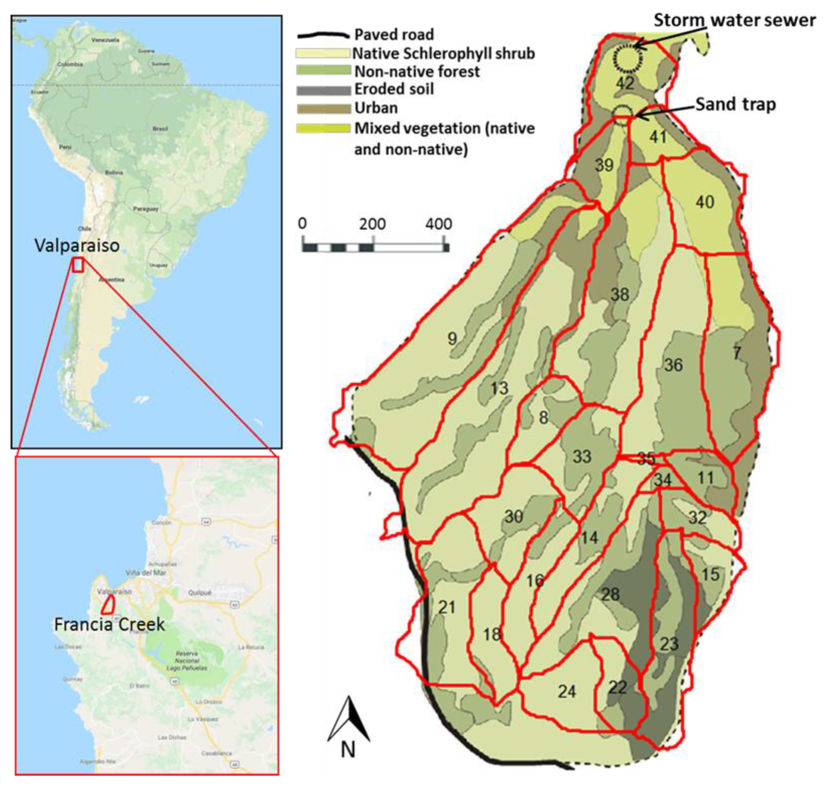
The city of Valparaiso is located in the central region of Chile. Its topography is dominated by 39 creeks (that drain waters from 44 hills that surround the city). The creeks were formed by natural terrain abrasion resulting from precipitation events. The region is characterized by dry weather, with few but intense precipitation events occurring mainly in the winter season (June–August). Baseflow erosion of the silty-clay soil, and oxidation of the granite rock that supports the soil layers also contribute to sediment concentrations and loading in the streams. The waters drained by the creeks feed the storm water pipes of the city system where sediment deposition has been a recurring problem requiring costly infrastructure implementation to remediate the situation [12]. One of the creeks that has been identified as critical is Francia Creek (Figure 1).

Francia Creek (Figure 1) watershed covers approximately 3.24 km² [12]. Land cover within the catchment consist mainly of native and exotic vegetation, eroded soil, and urban areas. Soils in the Francia Creek catchment consist of weathered sedimentary rock (sand, clay, and silt) with a thin organic top layer [20]. The instability of these materials makes the watershed side slopes susceptible to mass removal processes, mainly because the sedimentary rock expands and mobilizes when rainfall increases [21]. Hillslopes are steeper than 40% and they are prone to erodible processes and mudslides during the rainy season. Water flow in the creek can be strong enough to suspend particles in the water column and transport them downstream. To avoid the sediment entering the stormwater sewer network, a sand trap was built at the lowest point of the catchment area (Figure 2). The sand trap accumulates up to 1500 m³ of sediment annually. The accumulated sediment is cleaned up once a year and disposed in a sanitary landfill. Figure 2A shows the upstream side of the sand trap soon after it was cleaned up of debris. Figure 2B shows the sand trap almost full of debris and sediments after a series of strong precipitation events.

Since the erodible processes that have characterized Francia Creek watershed will continue to occur in the future (due to urban growth and other human activities) quantifying the risk associated with high sediment loading events would allow the development of early-warning systems that minimize damage. The initial step in the development of a warning system is building effective forecasting tools.

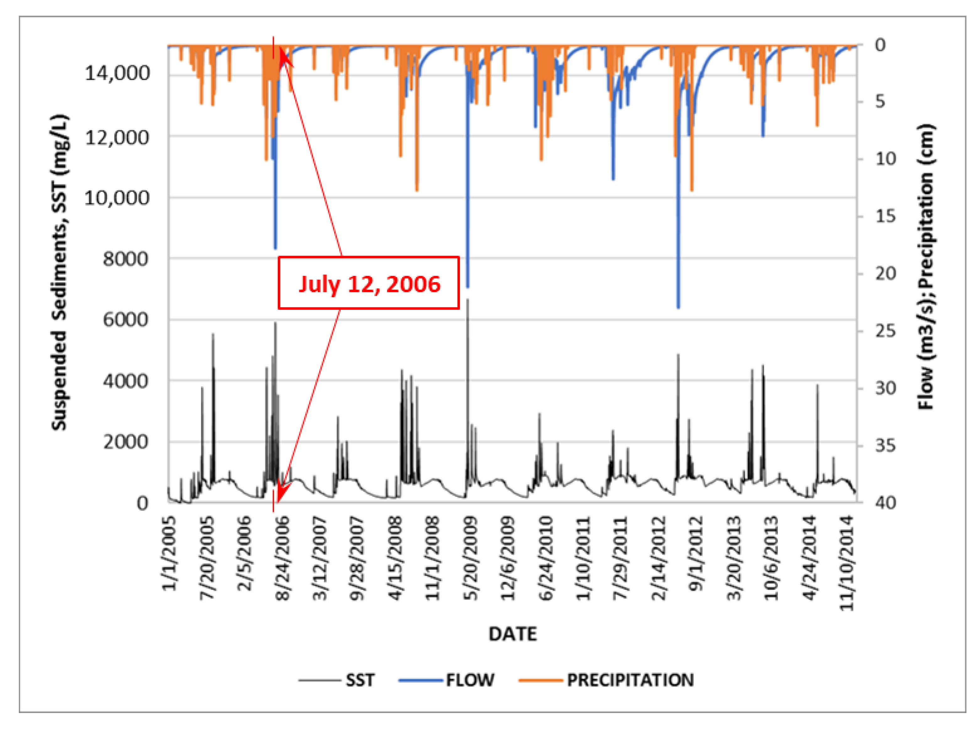
Alarcon and Magrini [12] performed measurements and daily estimations of precipitation, flow, and total suspended sediment concentrations (SST) for Francia Creek watershed at the upstream section of the sand trap (Figure 3). The figure shows that SST concentrations follow a seasonal pattern—concentration peaks occur during the rainy season (June to August). SST concentration peaks fluctuate within 1500 to 6660 mg/L and take place after or during daily precipitation events. Rainfall events accumulating 50 mm to 127 mm produce peak streamflow ranging from 8 m³/s to 23 m³/s. It should be noted that those peaks are preceded by lower intensity precipitation events in days previous to the peak events. Figure 3 also shows measured and estimated SST concentrations corresponding to days when there was absence of rainfall and Francia Creek only carries baseflow (water seeping into the stream from the vadose zone even in the absence of rain). Concentrations ranging between 200 mg/L to 350 mg/L correspond to baseflows ranging between 3 L/s to 5 L/s. Baseflow is continuous throughout the year.

Figure 4 illustrates the dependence of SST concentrations on antecedent conditions of precipitation and flow and follows a discussion on a mudflow event that took place at Francia Creek watershed, on 12 July 2006. SST, flow, and precipitation data for dates 4 July 2006 to 26 July 2006 are shown. On 10 July 2006, a strong precipitation event (200 mm) generated flows of up to 9.93 m³/s and SST concentrations of 4770 mg/L. The day after (11 July 2006), the rain continued to fall accumulating 53 mm of precipitation at the end of the day, generating flows of up to 9.90 m³/s and SST concentrations of up to 4320 mg/L. On 12 July 2006, it did not rain, but mudflow (generated in Francia Creek watershed) produced injuries to five people and damaged several cars in areas close to the watershed exit. In total, twenty people had to be evacuated. Two weeks later (24 July 2006), a precipitation event of almost 160 mm, that produced flows of up to 18 m3/s and SST concentrations of 5920 mg/L, did not produce consequences. The difference in this latter event was that precipitation intensity in days before and after the event was much milder than the recorded peak precipitation of 160 mm. Therefore, the antecedent conditions (rainfall and soil status) in days previous to the peak precipitation event, as well as rainfall and flow occurring in the following day, strongly influenced the generation of the mudflow incident.

The analysis above illustrates the challenges for predicting or forecasting time-series of SST concentrations and loadings. The strategies and methodologies for forecasting SST events should be able to account for antecedent precipitation, flow, and SST concentrations before the occurrence of a peak SST loading or concentration event.

2.2. Forecasting or Predicting SST Time-Series

Estimating or predicting SST time-series in rivers, lakes, or estuaries is usually performed through hydrological and water quality modeling. Nevertheless, there are other quantitative approaches developed and oriented towards specific objectives. Event-based models use simpler formulations for rainfall-runoff generation [22] but are usually developed for short-term purposes such as flood/flow forecasting and/or infrastructure designing. Other approaches that do not require information regarding the physical process (such as non-parametric algorithms) constitute an alternate method. Continuous non-parametric hydrological models were shown to be particularly useful for long-term water resources management (e.g., estimation of design flows, land-use change impacts, and effects of climate change). Non-parametric models such as antecedent precipitation indices, regression, artificial neural networks, fuzzy logic, and frequency analysis were used extensively [22].

The artificial neural network (ANN) approach to time-series prediction is a non-parametric method. For simple non-linear functions of one or several independent variables ANN are universal interpolators, but simple ANN configurations have limitations in modeling seasonal patterns. Special configurations of ANN have been used with success to predict flows and sediment concentrations for rivers around the world [15]. The most commonly used models are artificial neural networks with dynamic architecture (DANN), autoregressive neural networks (ARNN), non-linear autoregressive exogeneous neural networks (NARX), or hybrid configurations that combine ANN with other modeling approaches. Examples of those ANN configurations that reported good predictions of streamflow under flood and drought conditions are found in [23,24,25,26]. Similarly, ARNN and DANN were used extensively for estimating sediment concentrations (e.g., [27,28,29,30]). However, in most of those ANN applications the validation period of the model output corresponded to within-year or seasonal events because the input data was partitioned to capture the seasonality dependence of the input time-series. Also, some of those research projects scaled the input data for improving predictions. There are no ANN model applications that simulate continuous daily SST estimations for a whole year, using raw (not scaled) input data. Due to the strong non-linear SST response to precipitation and flow, non-linear autoregressive architectures with exogenous inputs (NARX ANN) seem to be the most appropriate for predicting SST concentrations if continuous daily estimations are desired, provided that exogenous data are used to capture antecedent hydrological conditions.

2.3. Selection of Model Architecture

The NARX network is a dynamical neural architecture commonly used for nonlinear dynamical systems. When applied to time-series prediction, the NARX network is designed as a feedforward time-delayed neural network (TDNN). 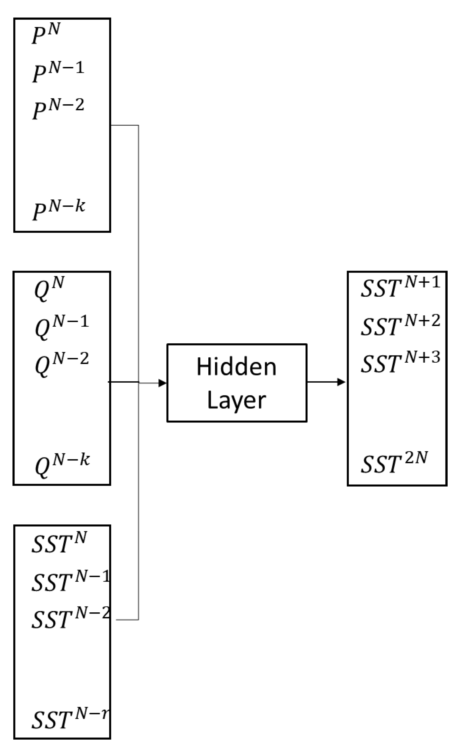NARX neural networks are recurrent dynamic networks, provided with feedback connections which enclose at least two layers of the network, and can use past values of predicted or true (measured) time-series [31]. In this research, a NARX configuration, is proposed, in which past values of the SST time-series, past values of the driving time-series (precipitation and flow), and current precipitation and flow time-series (exogeneous input) are used to perform the SST concentration forecast.

2.4. Determination of Model Structure

To forecast a total suspended sediments time-series of size N ($SS{T}^{N+i}, i:1, 2, 3,\dots ..N$) using a NARX net, based on three time-series that contain past precipitation (P), flow (Q), and total suspended sediments (SST) data ($P^i, Q^i, SS{T}^i, i:1, 2, 3,\dots \dots N$), there are important ANN specifications that have to be predetermined. There are two types of NARX architectures—closed-loop NARX architecture in which prediction of total suspended sediments is done from the present and past measured values of precipitation and stream flow, and the past predicted values of total suspended sediments and open-loop architecture, in which the future value of total suspended sediments,$SS{T}^{N+i}$, is predicted from the observed present and past values of precipitation ($P^{N-k}$), and stream flow ($Q^{N-k}$), and the observed past values of total suspended sediments ($SS{T}^{N-r}$). In this research, an open-loop NARX net was used. In the above equations, k and r are the input and feedback delays, respectively, and represent the number of time-series data that are used (from each input time-series data) to perform the forecast with the calibrated open network. Figure 5 presents a conceptual description of the NARX net used in this research.

The reason for using an open network is to avoid uncertainty propagation. In other fields of research where data uncertainty in the observed data is low, an open loop NARX is used to train the network, and then a closed-loop architecture (in which the network generates a forecast using the predicted data as the feedback input) is used for forecasting [32]. However, since observed SST time-series data are usually measured indirectly via turbidity samplers that allow estimation of SST concentrations, they have an important (but acceptable) degree of uncertainty [33]. Forecasting SST concentration values using NARX-forecasted SST concentrations (as it is done in closed NARX nets) may result in unnecessary propagation of the inherent uncertainty of observed SST data.

In this research, forecasting of SST concentrations was performed without scaling the input data. Efforts were put on forecasting daily SST concentrations for extended periods of time (N > 365). However, forecasting of monthly mean and monthly maximum concentrations was also performed using the developed NARX network. All computations were performed using MATLAB.

The narxnet MATLAB function, with input and feedback delays, open feedback mode, and Bayesian regularization training algorithm (trainbr), was used. Bayesian regularization is a mathematical method that converts a nonlinear regression into a “well-posed” statistical problem by minimizing a linear combination of squared errors and weights [34]. The resulting ANN is neither overtrained nor overfit, with a reduced number of effective network parameters or weights, considerably smaller than the number of weights in a standard fully connected back-propagation neural net [34].

2.5. Input Data Selection and Data Splitting

In order to explore the effect of training data size to achieve a successful prediction of SST, the number of years for training and prediction was varied.

Table 1. Training data size and splitting.

Model Run	Number of Years Used for Training			Number of Years Used for Forecasting
	Precipitation	Flow	SST	Precipitation	Flow	Predicted SST
Initial	2005–2012	2005–2012	2005–2012	2005–2012	2005–2012	2013–2014
Final	2011–2012	2011–2012	2011–2012	2011–2012	2011–2012	2013–2014

details the process.

Initially, precipitation ($P^i$), flow data ($Q^i$), and total suspended sediment concentrations ($SS{T}^i$) data from years 2005 to 2012 were used for training the NARX net. Several combinations of yearly datasets were tested until optimal statistical indicators of fit between simulated and observed daily SST concentrations data were achieved. The final training data set ($P^{N-k}$, $Q^{N-k}$, and $SS{T}^{N-r}$) corresponded to years 2011 and 2012 with respective input delay, k, and feedback delay, r, which are discussed in subsequent sections of this paper. For the prediction phase, data from years 2011 through 2012 were used to predict total suspended sediments, $SS{T}^{N+i}$, for years 2013 and 2014. To account for antecedent conditions of precipitation and flow, $P^{N+i-1}$ and $Q^{N+i-1}$, data (corresponding to the forecasted years) was used as exogenous input.

2.6. Model Calibration and Validation

After adopting the type of neural network (NARX) and developing a strategy for data-splitting, the ANN network was calibrated with several values and combinations of number of neurons in hidden layer, number of hidden layer nodes, and number of iterations. Other NARX net parameters were also varied in the training process. Input and feedback delays partitioned the input time-series data into subsets, during the computation of the forecasted SST time-series. Physically they represented the set of past precipitation, flow, and SST data values that determined the forecasted SST concentration. In MATLAB, input delays could range from 0 to N, while the range of feedback delays is 1 to N. By exploring the behavior of the observed data through time, initial numerical values of input and feedback delays were determined. From the initial estimation of the delay values, a heuristic approach was followed until obtaining a calibrated NARX net. In this research, input delays were varied from 1:15 to 1:60 and feedback delays from 1:2 to 1:6 (MATLAB notation for these parameters is used).

During NARX training, the general practice is to divide the data into three subsets—a training set (used for computing the gradient and updating the network weights and biases), a validation set (for comparing NARX generated output to the validation set), and a test set (that provides an additional check on que quality of the NARX output) [35]. Nevertheless, since in this research an actual validation of the NARX model was performed with observed SST time-series data that were independent from the time-series used during training, the preliminary validation that MATLAB performs was used only as an indicator of the ANN training quality. In this context, training set ratios were varied from 1/60 to 1/95, validation set ratios from 1/5 to 1/40, and test ratios from 1/5 to 1/20 (MATLAB notation for these parameters is used).

Statistical indicators of fit between forecasted and observed data and corresponding statistical errors were computed to quantify the quality of simulated data. The following indicators were used for assessing statistical fit: coefficient of determination (R²); Nash–Sutcliffe coefficient (NS), Kling-Gupta efficiency index (K-G), and Willmott’s index of agreement (d). The root-mean-squared-error to standard deviation ratio (RSR) was calculated to quantify statistical errors, and percent bias (PBIAS) was computed to determine the bias of simulated data with respect to observed data [25].

Table 2. Formulae for calculation of indicators of statistical fit, error, and bias. The table includes acceptability ranges for daily-step simulations.

Indicators of Fit	Formulae	Range
Root-mean-squared-error to standard deviation ratio, $RSR=\frac{RMSE}{STDE{V}_{Obs}}$	$\frac{\sqrt{{{\displaystyle \sum }}_{i=1}^n\left(Y_i^{Obs}-Y_i^{Sim}\right){.}^2}}{\sqrt{{{\displaystyle \sum }}_{i=1}^n\left(Y_i^{Obs}-Y_i^{Mean}\right){.}^2}}$	RSR < 0.79
Percent bias, PBIAS	$\frac{{{\displaystyle \sum }}_{i=1}^n\left(Y_i^{Obs}-Y_i^{Sim}\right)\ast 100}{{{\displaystyle \sum }}_{i=1}^n\left(Y_i^{Obs}\right).}$	−18% < PBIAS < 18%
Correlation coefficient, R	$\sqrt{\frac{{{\displaystyle \sum }}_{i=1}^n\left(Y_i^{Sim}-Y_i^{Mean}\right){.}^2}{{{\displaystyle \sum }}_{i=1}^n\left(Y_i^{Obs}-Y_i^{Mean}\right){.}^2}}$	R > 0.71
Coefficient of determination	$R^2$	$R^2$> 0.50
Nash–Sutcliffe efficiency, NS	$1-\frac{{{\displaystyle \sum }}_{i=1}^n\left(Y_i^{Obs}-Y_i^{Sim}\right){.}^2}{{{\displaystyle \sum }}_{i=1}^n\left(Y_i^{Obs}-Y_i^{Mean}\right){.}^2}$	NS > 0.50
Kling-Gupta efficiency, K-G	$1-\sqrt{{\left(\frac{Y_{Sim}^{Mean}}{Y_{Obs}^{Mean}}-1\right)}^2+{\left(\frac{STDE{V}_{Sim}}{STDE{V}_{Obs}}-1\right)}^2+{\left(R-1\right)}^2}$	K-G > 0.50
Willmott’s index of agreement, d	$1-\frac{{{\displaystyle \sum }}_{i=1}^n\left(Y_i^{Obs}-Y_i^{Sim}\right){.}^2}{{{\displaystyle \sum }}_{i=1}^n\left(\left|Y_i^{Sim}-Y_{Obs}^{Mean}\right|+\left|Y_i^{Obs}-Y_{Obs}^{Mean}\right|\right){.}^2}$	d > 0.65
$Y_i^{Obs}=\mathrm{Observed} \mathrm{SST} \mathrm{concentration}$ $Y_i^{Sim}=$ Simulated SST concentration $Y_{Obs}^{Mean}=\mathrm{Mean} \mathrm{of} \mathrm{observed} \mathrm{SST} \mathrm{concentration}$ $Y_{Sim}^{Mean}=\mathrm{Mean} \mathrm{of} \mathrm{simulated} \mathrm{SST} \mathrm{concentration}$, $n=$ Total number of daily SST concentrations

summarizes the statistical indicators used.

Model validation was performed at daily and monthly levels. The hindcasting and forecasting capabilities of the NARX net was assessed. The acceptable ranges or threshold values of the statistical indicators were defined after thorough review of the literature.

Moriasi et al. [36] states that if the statistical fit indicators (for monthly SST simulations) are within the following ranges, the simulation is satisfactory: RSR < 0.70, −30% < percent bias (PBIAS) < 55%, R² > 0.5, and NS > 0.50. However, the statistical indicators’ ranges need to be modified appropriately for shorter simulation time-steps. It is recommended to extend the acceptability ranges corresponding to monthly simulations by 20% to apply them to daily simulations. [36]. Nevertheless, the literature shows that the modeling community reports much wider and flexible ranges when assessing the quality of simulated data, which reflects the degree of difficulty on modeling and simulating SST concentrations. The following NS ranges for daily sediment concentration simulations are reported in Moriasi et al. [36]: −2.5 < NS < 0.11 for calibration and −3.51 < NS < 0.23 for validation. The following ranges were found by Ang and Oeurng [26]: NS > 0.38, PBIAS < 5.1%, and RSR < 0.79, for calibration. For validation: NSE > −6.61, PBIAS < −78.38%, and RSR < 2.67 are reported [37]. Kling-Gupta efficiencies within the range 0.5 < K-G < 1.0 are usually considered acceptable ([38].

In this research, the acceptability ranges for the indicators of statistical fit (NS, R², and K-G) were set up so that the prediction capabilities of the NARX model are better than satisfactory. The upper limit for the estimators of fit is 1.0, corresponding to perfect fit between simulated and observed data. On the other hand, correlation coefficient values greater than 0.7 are considered acceptable (R > 0.7); therefore, the acceptability range for the coefficient of determination would be: R² > 0.5. Moreover, Knoben et al. [38] (after performing a random sampling experiment) report that K-G = 0.5 correspond (in average) to NS = 0.5. Based on these considerations, Table 2 shows the statistical indicators acceptability ranges and formulae used in this research.

Summarizing, the quality of the NARX output was categorized as having good statistical fit with observed data according to the following criteria:

• Monthly time-step simulations: RSR < 0.7, −15% < PBIAS < 15%, R² > 0.6, NS > 0.6, and K-G > 0.6.
• Daily time-step simulations: RSR < 0.79, −18% < PBIAS < 18%, R² > 0.5, NS > 0.5, and K-G > 0.5.
• In cases in which simulations for SST produced unbalanced performance ratings, the Willmott’s index of agreement (d) was calculated, and if most statistical indicators were on the acceptable ranges, the simulation was rated “satisfactory”. Since in this research, d is used as a deciding qualifier of statistical fit, its threshold values of acceptability are more stringent than those of R² and NS indicators–for monthly simulations d > 0.78 and for daily simulations d > 0.65.
• Ranges for PBIAS and RSR were assigned after [36].

3. Results

3.1. NARX Training

Training of the NARX net was a trial-and-error process, as in any hydrological model calibration methodology. Daily precipitation, flow, and SST data for years 2011 and 2012 were used for calibration. The network architecture (number of nodes and hidden layers) was modified sequentially, along with several combinations of other training parameters. The number of nodes in the hidden layer was varied within the range of 5 to 100. Similarly, the number of iterations was varied from 50 to 1000. Other NARX net parameters were also varied in the training process—input delays were varied within the 1:15 to 1:60 range. The ranges of variation for feedback delays were from 1:2 to 1:6. Training set ratios were varied from 1/60 to 1/95, validation set ratios from 1/5 to 1/40, and test ratios from 1/5 to 1/20.

Table 3. Training data size and splitting.

Non-Linear Autoregressive Exogenous Neural Network (NARX) Feature	Adopted Value
Number of layers	3 (input, hidden, output)
Number of nodes in hidden layer	12
Architecture	Open loop
Number of iterations	100
Input delays	1:30
Feedback delays	1:3
Train ratio	70/100
Value ratio	15/100
Test ratio	15/100
Training algorithm	Bayesian regularization

summarizes the final values adopted for all training parameters. MATLAB notation for all parameters is used.

3.2. Calibration Results

As stated in previous sections, daily precipitation, flow, and SST data for years 2011 and 2012 were used for training of the neural network. Figure 6 illustrates the good quality results achieved during this model development phase. The figure compares simulated daily SST data to observed daily SST data (from 1 January 2011 to 31 December 2012), at the Francia Creek watershed exit. Scatter plots of measured versus simulated data are also shown, including statistical fit parameters (NS, PBIAS, RSR, R², and K-G).

Figure 6 shows that the trained NARX successfully captured seasonal SST trends, peak values and daily baseflow SST concentrations.

Table 4. NARX net calibration/training results.

Comparison Period	Indicator Ranges for Daily SST Simulation
	RSR < 0.79	−18% < PBIAS < 18%	R2 > 0.5	NS >0.5	K-G > 0.5
2011	0.26	−0.28%	0.94	0.93	0.94
2012	0.32	9.99%	0.94	0.90	0.88

shows that training of the NARX net (with daily data from years 2011 and 2012) was successful. All the statistical indicators are shown to be well within acceptable ranges for daily simulations. Consequently, the simulated output has a particularly good statistical fit with the observed data. Nevertheless, results during training of a neural network are usually characterized by good indicators of statistical fit and low statistical error. The actual test of a neural network is during the validation phase, in which the NARX predictions are compared to independent datasets of observed SST concentrations.

3.3. Validation Results

Validation of the neural network was undertaken in two steps: (a) assessing its capability to hindcast past observed data for years 2008 through 2010 (daily baseflow, monthly mean, and monthly maximum SST concentrations) and, (b) evaluating its potential to forecast daily SST concentrations, and monthly maximum and monthly mean SST concentrations.

3.3.1. Hindcasting SST Concentrations

Figure 7 shows simulated SST concentrations for daily baseflow during years 2008 and 2010. The scatter plots associated with the daily comparison charts for SST concentrations and

Table 5. Hindcasting of daily SST concentrations for years 2008–2010.

Comparison Period	Indicator Ranges for Daily SST Simulation
	RSR < 0.79	−18% < PBIAS < 18%	R2 > 0.5	NS > 0.5	K-G > 0.5
2008–2010	0.51	−13.40%	0.82	0.74	0.83

, show that the neural network provided particularly good quality hindcasting of daily baseflow SST concentrations. All statistical indicators of fit were greater than 0.73 (NS = 0.74 R² = 0.82, K-G = 0.83). Error indices (PBIAS and RSR) were also optimal—percent bias (PBIAS) was smaller than 14% and RSR (root mean square error normalized by the standard deviation of observed concentrations) was smaller than 0.52. Therefore, the neural network is able to hindcast concentration values occurring in Francia Creek under baseflow conditions (i.e., absence of rain).

The NARX net capability of hindcasting mean and maximum concentrations was explored at monthly time-step. Figure 8 shows comparison charts of simulated and observed monthly mean and maximum SST concentrations. The neural net acceptably hindcasts the monthly mean SST concentrations.

Table 6. Hindcasting of monthly mean and maximum SST concentrations for years 2008–2010.

Monthly SST for 2008–2010	Indicator Ranges for Monthly SST Simulation
	RSR < 0.70	−15% < PBIAS < 15%	R2 > 0.6	NS > 0.6	K-G > 0.6
Mean	0.74	−15.24%	0.64	0.55	0.72
Maximum	0.55	1.52%	0.69	0.69	0.71

summarizes the statistical fit and error indicators for the monthly simulations.

Table 6 shows that monthly mean SST concentrations hindcasted by the NARX net for years 2008 to 2010 are acceptable. Statistical indicators of error and bias (RSR and PBIAS) are slightly off from the acceptable ranges, but the statistical indicators of fit efficiency and correlation are good (R² = 0.64, NS = 0.55, K-G = 0.72). However, since NS is slightly lower than the required minimum value (Table 6), the Willmott’s index of agreement is calculated to further ascertain on the statistical fit of the simulated SST concentrations. The resulting index of agreement is d = 0.86 which confirms the good quality of the monthly SST mean concentrations forecasting.

The neural network estimations for monthly maximum SST concentrations are very good. RSR = 0.55 indicates low RMSE or residual variation and therefore an accurate model simulation. Similarly, PBIAS = 1.52% indicates a low biased model simulation, with simulated data slightly overestimating observed data. The statistical indicators of fit (R² = 0.69, NS = 0.69, and K-G = 0.71) categorize the NARX net output as a good estimation of monthly maximum SST concentrations. Therefore, the neural network performance in hindcasting was successful.

3.3.2. Forecasting SST Concentrations

The NARX net forecasting capabilities was initially assessed for monthly maximum and monthly minimum SST concentrations, to verify if the neural network was proficient in capturing seasonal concentration trends and values. The evaluation included the comparison of simulated and observed data for two years hindcasts—2013 and 2014. Predicting seasonal and interannual variation in SST concentrations is key in the understanding of erosion and sediment transport processes at watershed scale. Depending on the season of the year, weathering could be more important than sediment transport, and vice versa.

Figure 9 and

Table 7. Forecasting of monthly mean and maximum SST concentrations for years 2013–2014.

Monthly SST for 2013–2014	Indicator Ranges for Monthly SST Simulation
	RSR < 0.70	−15% < PBIAS < 15%	R2 > 0.6	NS > 0.6	K-G > 0.6
Mean	0.79	3.29%	0.43	0.34	0.65
Maximum	0.62	18.87%	0.69	0.60	0.54

show a comparison of NARX-estimated monthly SST concentrations for years 2013 and 2014. As shown, monthly mean SST concentrations estimations are barely acceptable. Statistical errors for monthly mean estimations are contradictory—while PBIAS = 3.29% indicates low deviation from observed data, RSR = 0.79 shows that the normalized root mean square error is slightly higher than the desired range (RSR < 0.7). The statistical indicators of fit are also contradictory. While the Kling-Gupta efficiency value indicates good fit (K-G = 0.65), the coefficient of determination R² = 0.43 is not satisfactory. To settle this apparent contradiction, the Willmott’s index of agreement, d, was calculated. The computation of this statistical indicator of fit produced a value of d = 0.79, indicating good fit between simulated and observed SST concentrations. If simulation for one output variable produces unbalanced performance ratings (as in this case), then, the overall performance should be described conservatively as satisfactory [25].

On the contrary, forecasting of monthly maximum SST concentrations is shown to be successful (Table 7, Figure 9). Only PBIAS is slightly higher than the required threshold (15%) and Kling-Gupta is slightly below 0.6. All other statistical (RSR, R², and NS) indicators are within the acceptable ranges. The statistical fit of simulated SST concentrations to observed data is further reinforced by the calculation of the Willmott’s index of agreement—d = 0.84 (indicating good statistical fit). Therefore, the NARX model is able to forecast the monthly maximum SST concentrations for years 2013 and 2014.

Forecasting of SST concentrations for years 2013 and 2014 was also performed at daily time-step. Figure 10 shows a comparison of daily simulated SST concentrations to daily observed SST data. A scatter plot of observed versus simulated data is included, showing statistical indicators of error and fit for the simulated SST concentrations.

Table 8. Forecasting of daily SST concentrations for years 2013–2014.

Comparison Period	Indicator Ranges for Daily SST Simulation
	RSR < 0.79	−18% < PBIAS < 18%	R2 > 0.5	NS > 0.5	K-G > 0.5
2013–2014	0.89	3.41%	0.28	0.21	0.50
2014	0.91	−15.86%	0.53	0.47	0.60
Baseflow	0.54	3.6%	0.73	0.71	0.84

summarizes error and fit statistical indicators obtained for the simulated daily SST concentrations, comparing them to acceptable ranges for daily level. The statistical indicators of fit are contradictory—while K-G has an acceptable value (0.5), R² and NS present values lower than the acceptable threshold. Indicators of statistical error are also in disagreement—PBIAS = 3.41 reveals low levels of bias, while RSR = 0.89 is higher than the acceptable value (0.79). As in previous cases, the Willmott’s index of agreement (d) was calculated for having more insight into the quality of simulated values. The resulting value is d = 0.68. Therefore, the daily forecasting of SST concentrations for years 2013 and 2014 is satisfactory.

If Figure 10 is explored further, it shows that the daily simulation of SST concentrations corresponding to 2014 approximates observed data better than in year 2013. Therefore, statistical indicators for 2014 were calculated separately. Table 8 shows the resulting values. As shown, statistical indicators of fit for year 2014 improved greatly (R² =0.53, NS = 0.47, K-G = 0.60). Moreover, the additional calculation of Willmott’s index of agreement yielded d = 0.82. Therefore, the statistical indicators for year 2014 reveal that forecasting for that year alone was of acceptable quality.

Forecasted daily SST concentrations for daily baseflow (during years 2013 and 2014) is shown in Figure 11. The figure and corresponding statistical indicators (Table 8) are shown to be very good. All statistical fit indicators are greater than 0.7 (R² = 0.73, NS = 0.71, K-G = 0.84). Likewise, indicators of statistical error are well below the acceptable maximum values—PBIAS = 3.6% < 15%, RSR = 0.54 < 0.79. Moreover, the NARX net is able to capture daily SST concentration peaks occurring during the period of analysis. Therefore, the forecasting of daily SST concentrations occurring under baseflow conditions is of very good quality.

4. Discussion

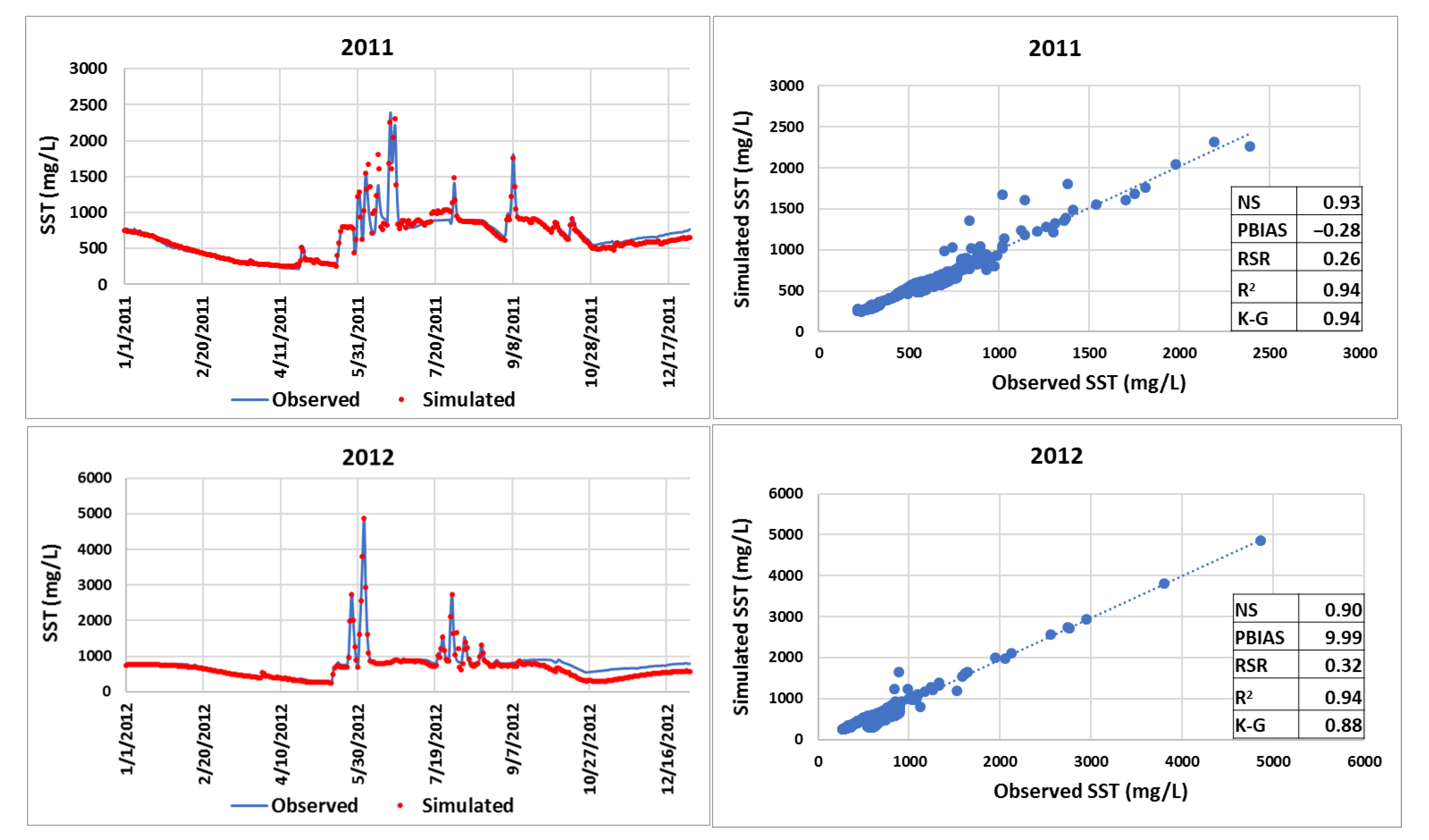
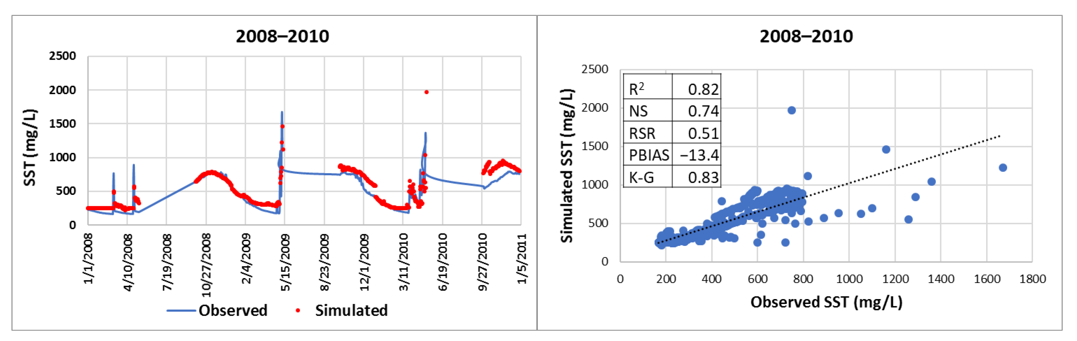
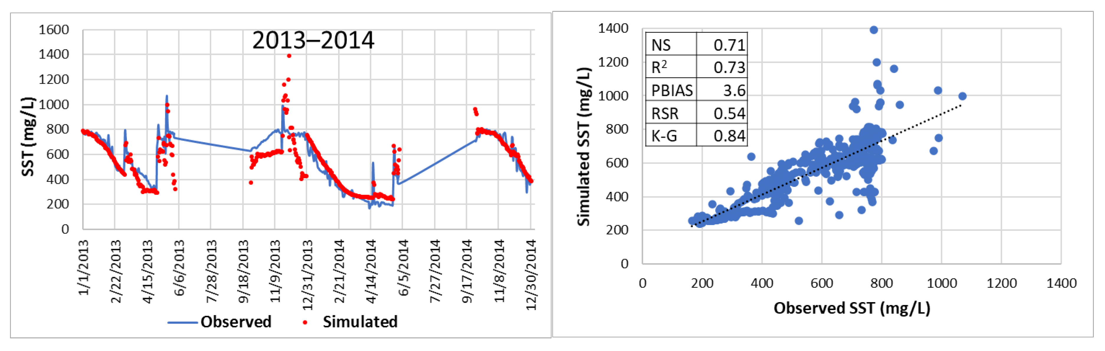
This research shows that forecasting total suspended sediment (SST) concentrations can be performed using a non-linear autoregressive artificial neural network with exogenous inputs (NARX). Although the modeling strategy and the resulting neural network were applied to estimate SST concentrations occurring at Francia Creek (Valparaiso, Chile), the NARX could be adjusted (via re-training) to estimate SST concentrations in other streams and watersheds. The NARX developed in this study was able to predict daily and monthly SST concentrations for years 2013 and 2014, based on precipitation and SST concentrations from previous years (2011 and 2012). The daily SST concentrations were more accurately forecasted for baseflow conditions. Indicators of statistical fit between forecasted and observed data were R² = 0.73, NS = 0.71, and K-G = 0.84, which indicate very good quality prediction levels of daily SST concentrations under baseflow conditions. Indicators of statistical error were below the acceptable maximum values—PBIAS = 3.6% < 15%, RSR = 0.54 < 0.79, which demonstrates that the simulated daily SST data had low residual variation and low bias, characteristics of accurate forecasting.

When comparing simulated and observed daily SST concentrations for a complete year, the NARX network produces a satisfactory forecasting of daily data. For year 2014, the statistical indicators of fit were R² = 0.53, NS = 0.47, K-G = 0.60, Willmott’s index of agreement d = 0.82. Therefore, the statistical indicators of fit were within acceptable margins. The forecasted SST concentrations underperformed in statistical error (RSR = 0.91 > 0.79) but overperformed bias indicators (PBIAS = −15.86% is within the range: −18% < PBIAS < 18%).

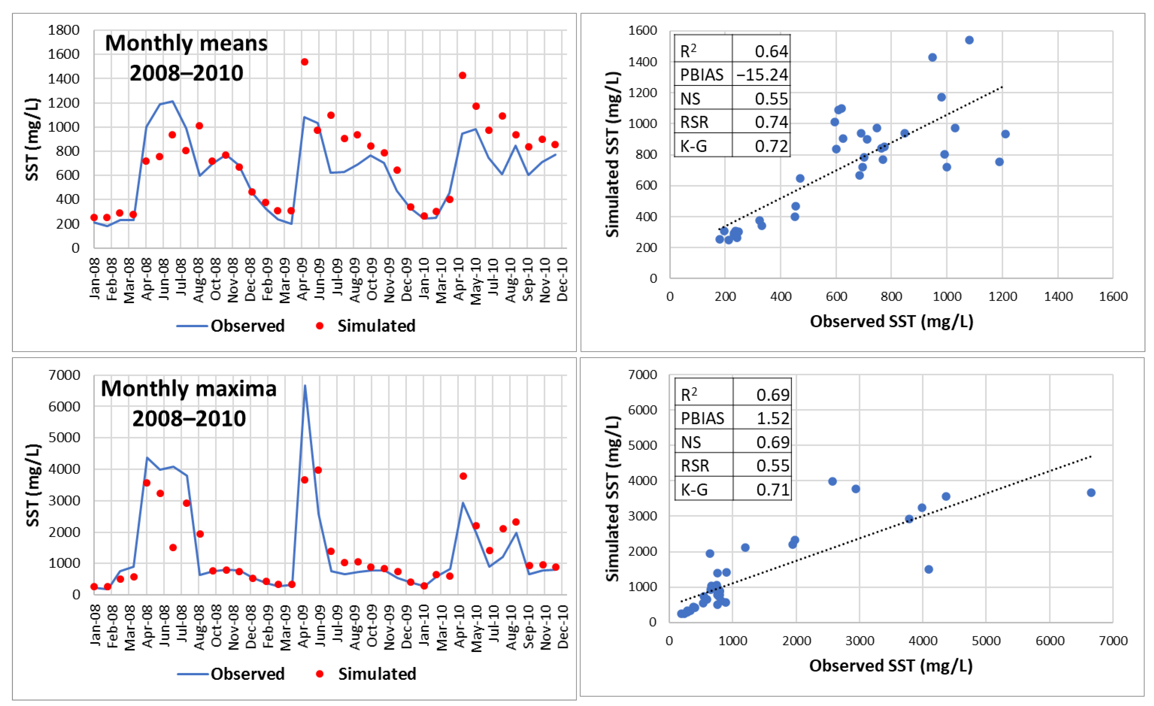
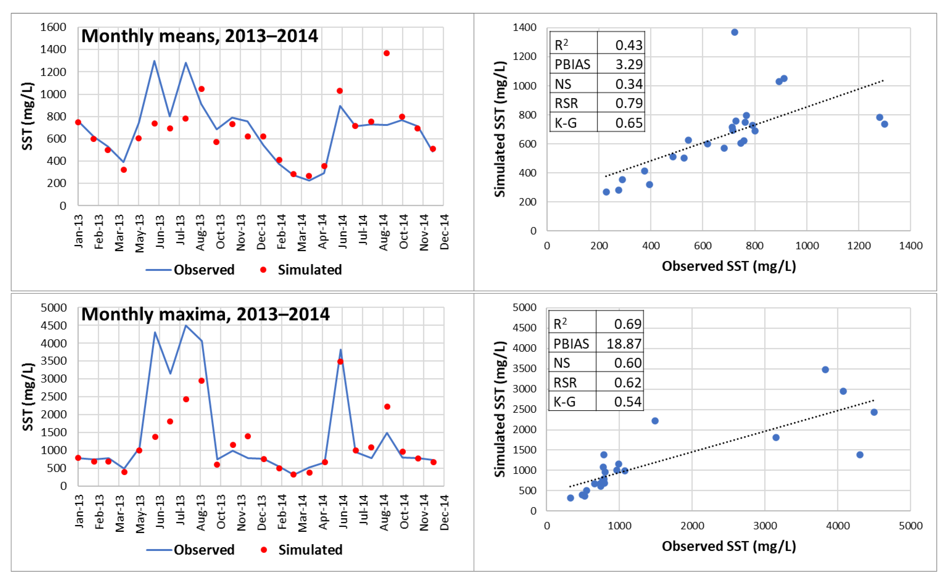
Predicting daily SST concentrations for two years decreases the forecasting quality of the neural network. Predictions for 2013 and 2014 yielded the following indicators of statistical fit: K-G = 0.5, R² = 0.28, NS = 0.21, Willmott’s index of agreement, d = 0.68. Indicators of statistical error were PBIAS = 3.41 (low bias), RSR = 0.89 > 0.79. Therefore, the daily forecasting of SST concentrations for years 2013 and 2014 was satisfactory. However, monthly maximum SST concentrations for the two-year period (2013 and 2014) were well captured by the NARX network: RSR = 0.62 > 0.6, PBIAS = 18.87% < 20%, R² = 0.69 > 0.6, NS = 0.60 > 0.6, K-G = 0.54 > 0.5, d = 0.84 > 0.8.

In consequence, the NARX network successfully forecasted daily SST concentrations for baseflow conditions for two years (2013 and 2014). Also, the neural network was able to forecast (within acceptable statistical fit margins) daily SST for up to one continuous year (2014). At a monthly level, the NARX network was able to predict maximum SST concentrations for two years (2013 and 2014).

The results reported in this paper are relevant to sustainable land management as they provide a forecasting methodology applicable to other watersheds. Nevertheless, the NARX-based forecasting model developed in this research is more site-specific than physically based models (such as the SWAT-MUSLE applications reported in [39]), and it may require substantial adjustments if meteorological conditions and flow regimes are very different to those encountered in this study.

References

1. Zhang, X.; Chen, X.; Liu, M.; Xu, Z.; Wei, H. Coupled changes in soil organic carbon fractions and microbial community composition in urban and suburban forests. Sci. Rep. 2020, 10, 1–12. [Google Scholar] [CrossRef]
2. Parlak, M.; Everest, T.; Ruis, S.J.; Blanco, H. Impact of urbanization on soil loss: A case study from sod production. Environ. Monit. Assess. 2020, 192, 1–12. [Google Scholar] [CrossRef] [PubMed]
3. Alarcon, V.J.; Sassenrath, G.F. Nitrate, Total Ammonia, and Total Suspended Sediments Modeling for the Mobile River Watershed. Int. J. Agric. Environ. Inf. Syst. 2017, 8, 20–31. [Google Scholar] [CrossRef]
4. Forecasting Pollutant Concentration in River to Protect Drinking Water Production. Available online: https://www.scopus.com/inward/record.uri?eid=2-s2.0-85093908096&partnerID=40&md5=5aacaeb5c86709e4ea5569591815ccc0 (accessed on 15 November 2020).
5. Tsai, L.-Y.; Chen, C.-F.; Fan, C.-H.; Lin, J.-Y. Using the HSPF and SWMM Models in a High Pervious Watershed and Estimating Their Parameter Sensitivity. Water 2017, 9, 780. [Google Scholar] [CrossRef] [Green Version]
6. Alarcon, V.J.; Johnson, D.; McAnally, W.H.; Van Der Zwaag, J.; Irby, D.; Cartwright, J. Nested Hydrodynamic Modeling of a Coastal River Applying Dynamic-Coupling. Water Resour. Manag. 2014, 28, 3227–3240. [Google Scholar] [CrossRef]
7. Alarcon, V.J. The Role of Boundary Conditions in Water Quality Modeling; Lecture Notes in Computer Science; Springer: Berlin, Germany, 2014; pp. 721–733. [Google Scholar] [CrossRef]
8. Yang, W.; Chen, H.; Xu, C.-Y.; Huo, R.; Chen, J.; Guo, S. Temporal and spatial transferabilities of hydrological models under different climates and underlying surface conditions. J. Hydrol. 2020, 591, 125276. [Google Scholar] [CrossRef]
9. Ji, L.; Wu, T.; Xie, Y.; Huang, G.; Sun, L. A novel two-stage fuzzy stochastic model for water supply management from a water-energy nexus perspective. J. Clean. Prod. 2020, 277, 123386. [Google Scholar] [CrossRef]
10. Dikshit, A.; Pradhan, B.; Alamri, A.M. Long Lead Time Drought Forecasting Using Lagged Climate Variables and a Stacked Long Short-term Memory Model. Sci. Total Environ. 2021, 755, 142638. [Google Scholar] [CrossRef]
11. Gormaz-Cuevas, D.; Riffo-Rivas, J.; Montastruc, L.; Brüning-González, M.; Díaz-Alvarado, F.A. A multi-objective optimization model to plan city-scale water systems with economic and environmental objectives: A case study in santiago, Chile. J. Clean. Prod. 2021, 279, 123737. [Google Scholar] [CrossRef]
12. Alarcon, V.J.; Magrini, C. Scenarios of Sediment Transport Management in Francia Creek; Lecture Notes in Computer Science, 10962; LNCS: Valparaiso, Chile, 2018; pp. 205–218. [Google Scholar] [CrossRef]
13. Aguas Andinas. Aguas Andinas Detalla Plan de Inversiones. 2017. Available online: https://www.aguasandinas.cl/noticias/historico-noticias/aguas-andinas-detalla-plan-de-inversiones (accessed on 15 November 2020).
14. Rajaee, T.; Jafari, H. Two decades on the artificial intelligence models advancement for modeling river sediment concentration: State-of-the-art. J. Hydrol. 2020, 588, 125011. [Google Scholar] [CrossRef]
15. Afan, H.A.; El-Shafie, A.; Mohtar, W.H.M.W.; Yaseen, Z.M. Past, present and prospect of an Artificial Intelligence (AI) based model for sediment transport prediction. J. Hydrol. 2016, 541, 902–913. [Google Scholar] [CrossRef]
16. Afan, H.A.; El-Shafie, A.; Yaseen, Z.M.; Hameed, M.M.; Mohtar, W.H.M.W.; Hussain, A. ANN Based Sediment Prediction Model Utilizing Different Input Scenarios. Water Resour. Manag. 2014, 29, 1231–1245. [Google Scholar] [CrossRef]
17. Ghose, D.K.; Samantaray, S. Modelling sediment concentration using back propagation neural network and regression coupled with genetic algorithm. Procedia Comput. Sci. 2018, 125, 85–92. [Google Scholar] [CrossRef]
18. Alp, M.; Cigizoglu, H. Suspended sediment load simulation by two artificial neural network methods using hydrometeorological data. Environ. Model. Softw. 2007, 22, 2–13. [Google Scholar] [CrossRef]
19. Wu, W.; Dandy, G.C.; Maier, H.R. Protocol for developing ANN models and its application to the assessment of the quality of the ANN model development process in drinking water quality modelling. Environ. Model. Softw. 2014, 54, 108–127. [Google Scholar] [CrossRef]
20. SERNAGEOMIN. Efectos del Incendio del 12 al 16 de abril de 201, Comuna de Valparaiso, Region de Valparaiso. Ministerio de Mineria, Santiago 2015. Available online: http://sitiohistorico.sernageomin.cl/pdf/volcanes/3-Efectos-del-incendio-del-12-al-16-de-abril-de-2014-en-la-comuna-de-Valparaiso.pdf (accessed on 15 November 2020).
21. Universidad Andrés Bello. Geomorfología Dinámica del Cajón del Maipo. 2015. Available online: https://www.geoaprendo.com/2014/12/informe-geomorfologia-dinamica-del.html. (accessed on 15 November 2020).
22. Xu, C.Y.; Xiong, L.; Singh, V.P. Black-Box Hydrological Models. In Handbook of Hydrometeorological Ensemble Forecasting; Duan, Q., Pappen-berger, F., Thielen, J., Wood, A., Cloke, H., Schaake, J., Eds.; Springer: Berlin/Heidelberg, Germany, 2017. [Google Scholar]
23. Nacar, S.; Hınıs, M.A.; Kankal, M. Forecasting Daily Streamflow Discharges Using Various Neural Network Models and Training Algorithms. KSCE J. Civ. Eng. 2017, 22, 3676–3685. [Google Scholar] [CrossRef]
24. Dariane, A.B.; Azimi, S. Streamflow forecasting by combining neural networks and fuzzy models using advanced methods of input variable selection. J. Hydroinformatics 2017, 20, 520–532. [Google Scholar] [CrossRef] [Green Version]
25. Daliakopoulos, I.N.; Tsanis, I. Comparison of an artificial neural network and a conceptual rainfall–runoff model in the simulation of ephemeral streamflow. Hydrol. Sci. J. 2016, 61, 2763–2774. [Google Scholar] [CrossRef]
26. Besaw, L.E.; Rizzo, D.M.; Bierman, P.; Hackett, W.R. Advances in ungauged streamflow prediction using artificial neural networks. J. Hydrol. 2010, 386, 27–37. [Google Scholar] [CrossRef]
27. Halecki, W.; Kruk, E.; Ryczek, M. Estimations of nitrate nitrogen, total phosphorus flux and suspended sediment concentration (SSC) as indicators of surface-erosion processes using an ANN (Artificial Neural Network) based on geomorphological parameters in mountainous catchments. Ecol. Indic. 2018, 91, 461–469. [Google Scholar] [CrossRef]
28. Meral, R. Analyses of turbidity and acoustic backscatter signal with artificial neural network for estimation of suspended sediment concentration. Appl. Ecol. Environ. Res. 2018, 16, 697–708. [Google Scholar] [CrossRef]
29. Sari, V.; Castro, N.M.D.R.; Pedrollo, O.C. Estimate of Suspended Sediment Concentration from Monitored Data of Turbidity and Water Level Using Artificial Neural Networks. Water Resour. Manag. 2017, 31, 4909–4923. [Google Scholar] [CrossRef]
30. Bhattacharya, B.; Van Kessel, T.; Solomatine, D.P. Spatio-temporal prediction of suspended sediment concentration in the coastal zone using an artificial neural network and a numerical model. J. Hydroinformatics 2012, 14, 574–584. [Google Scholar] [CrossRef] [Green Version]
31. Boussaada, Z.; Curea, O.; Remaci, A.; Camblong, H.; Mrabet, N.B. A Nonlinear Autoregressive Exogenous (NARX) Neural Network Model for the Prediction of the Daily Direct Solar Radiation. Energies 2018, 11, 620. [Google Scholar] [CrossRef] [Green Version]
32. Buitrago, J.; Asfour, S. Short-Term Forecasting of Electric Loads Using Nonlinear Autoregressive Artificial Neural Networks with Exogenous Vector Inputs. Energies 2017, 10, 40. [Google Scholar] [CrossRef] [Green Version]
33. Navratil, O.; Esteves, M.; Legout, C.; Gratiot, N.; Nemery, J.; Willmore, S.; Grangeon, T. Global uncertainty analysis of suspended sediment monitoring using turbidimeter in a small mountainous river catchment. J. Hydrol. 2011, 398, 246–259. [Google Scholar] [CrossRef]
34. Burden, F.; Winkler, D. Bayesian Regularization of Neural Networks. In Artificial Neural Networks; Livingstone, D.J., Ed.; Methods in Molecular Biology; Humana Press: Totowa, NJ, USA, 2008; Volume 458. [Google Scholar] [CrossRef]
35. Mathworks. Divide Data for Optimal Neural Network Training (r2020b). 2020. Available online: https://www.mathworks.com/help/deeplearning/ug/divide-data-for-optimal-neural-network-training.html;jsessionid=0322bf67b3599c9de6ef0bf5e7cc (accessed on 20 December 2020).
36. Moriasi, D.N.; Arnold, J.G.; Van Liew, M.W.; Bingner, R.L.; Harmel, R.D.; Veith, T.L. Model Evaluation Guidelines for Systematic Quantification of Accuracy in Watershed Simulations. Trans. ASABE 2007, 50, 885–900. [Google Scholar] [CrossRef]
37. Ang, R.; Oeurng, C. Simulating streamflow in an ungauged catchment of Tonlesap Lake Basin in Cambodia using Soil and Water Assessment Tool (SWAT) model. Water Sci. 2018, 32, 89–101. [Google Scholar] [CrossRef] [Green Version]
38. Knoben, W.J.M.; Freer, J.E.; Woods, R.A. Technical note: Inherent benchmark or not? Comparing Nash–Sutcliffe and Kling–Gupta efficiency scores. Hydrol. Earth Syst. Sci. 2019, 23, 4323–4331. [Google Scholar] [CrossRef] [Green Version]
39. Djebou, D.C.S. Assessment of sediment inflow to a reservoir using the SWAT model under undammed conditions: A case study for the Somerville reservoir, Texas, USA. Int. Soil Water Conserv. Res. 2018, 6, 222–229. [Google Scholar] [CrossRef]
Figure 1. Study area. Francia Creek watershed (covering 3.24 km2) is located in Valparaiso (Chile). Dry weather, with few, but intense, precipitation events in June–August, characterize the region. Native and non-native vegetation are predominant in the watershed. Slopes are greater than 40%.
Sustainability 13 00363 g001
Figure 2. Sand trap at Francia Creek watershed exit. (A) Sand trap after clean-up of upstream side. (B) Mudflow filling up the upstream side of the sand trap after a series of heavy rain events.
Sustainability 13 00363 g002
Figure 3. Historical data in Francia Creek watershed. Daily time-series of suspended sediments concentrations (SST), precipitation, and stream flow are shown (1 January 2005–31 December 2014). Sediment concentration peaks occur soon after intense and consecutive precipitation events.
Sustainability 13 00363 g003
Figure 4. Time-series of SST, precipitation, and stream flow for dates 4 July 2006 through 26 July 2006. A mudflow event occurred on 12 July 2020 after two consecutive rain events.
Sustainability 13 00363 g004
Figure 5. Conceptual description of the open-loop neural network used in this research. The future value of total suspended sediments,   S S T N + i , is predicted from observed present and past values of precipitation ( P N k ), and stream flow ( Q N k ), and the observed past values of total suspended sediments ( S S T N r ).
Sustainability 13 00363 g005
Figure 6. NARX training results. Daily SST concentrations and flow data for years 2011 and 2012 were used for training.
Sustainability 13 00363 g006
Figure 7. Hindcasting daily baseflow SST concentrations using the NARX net. The neural network successfully reproduced daily SST concentrations observed in daily baseflow in years 2008, 2009 and 2010.
Sustainability 13 00363 g007
Figure 8. Hindcasting using the NARX net. The estimations of the neural network are shown to be successful for monthly mean and maximum SST concentrations.
Sustainability 13 00363 g008
Figure 9. Forecasting of monthly mean and maximum for years 2013 and 2014. The neural network forecast of monthly maxima is shown to be successful while monthly means forecasting is less effective but acceptable.
Sustainability 13 00363 g009
Figure 10. Forecasting of daily SST concentrations for years 2013 and 2014. The statistical indicators for the NARX net forecast show that prediction of daily SST concentrations for 2013 and 2014 is limited. However, if 2014 is analyzed separately, the daily SST concentrations forecast is successful.
Sustainability 13 00363 g010
Figure 11. Forecasting daily SST concentrations for daily baseflow during years 2013 and 2014. The NARX net successfully predicts daily concentrations as reflected by the statistical indicators of fit, error and bias.
Sustainability 13 00363 g011