Deciphering Soil Spatial Variability through Geostatistics and Interpolation Techniques

 ,
,  and
and 
Abstract
1. Introduction
2. Materials and Methods
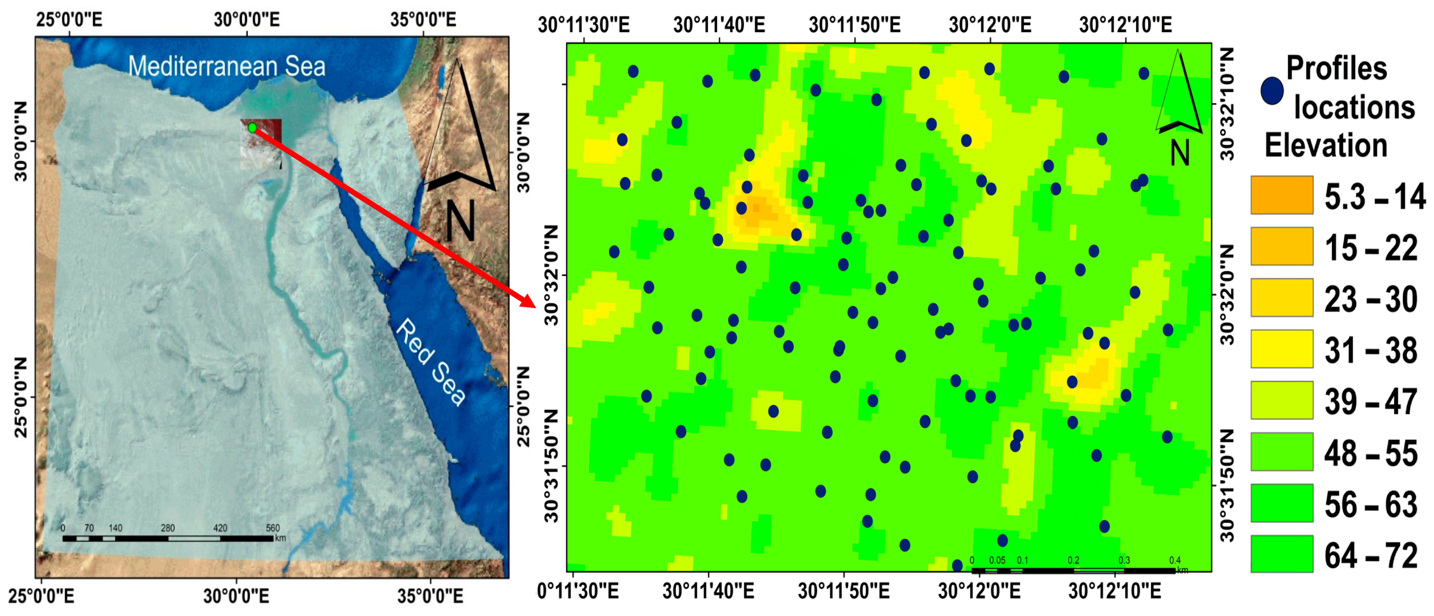
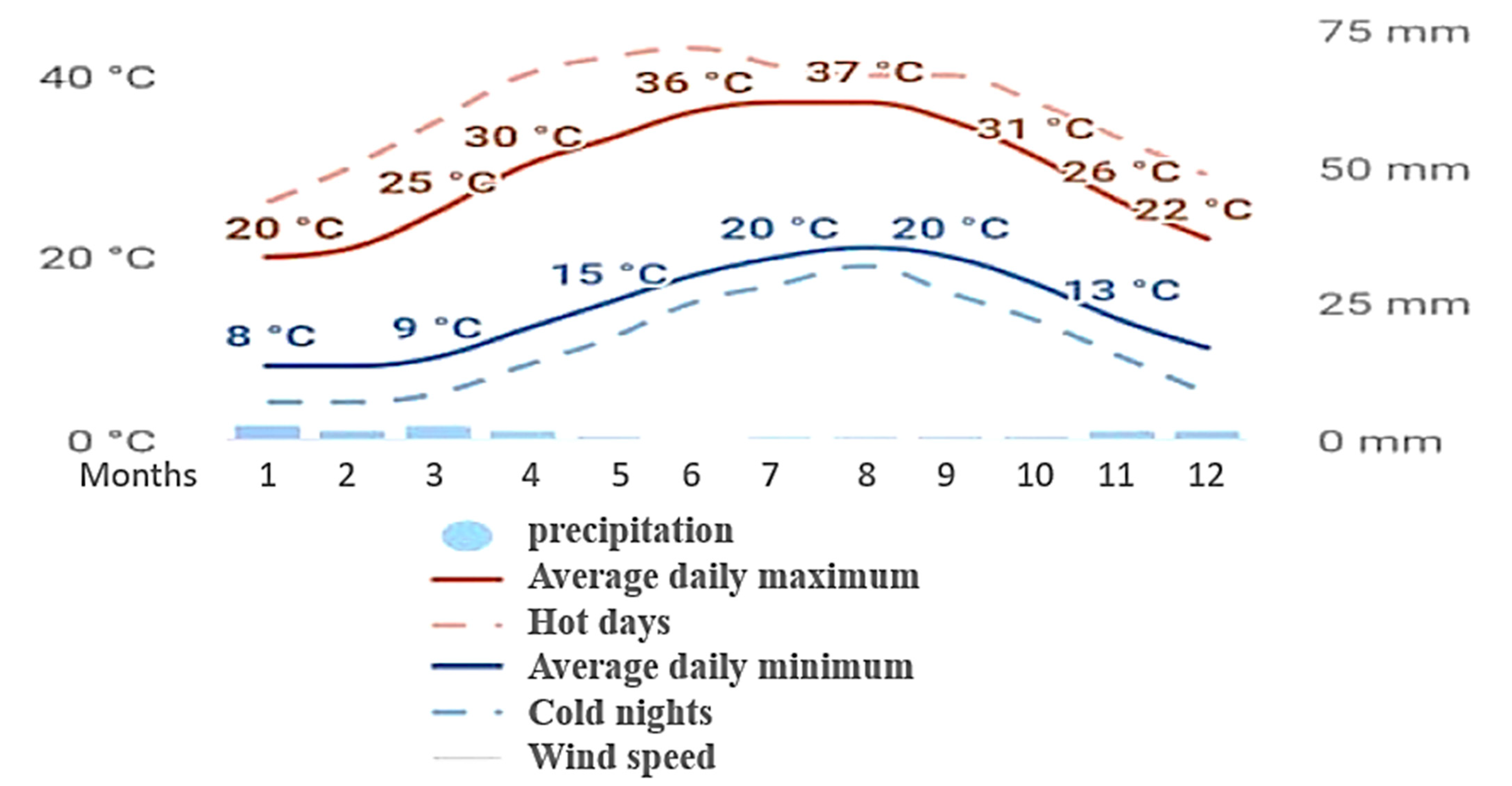
2.1. Study Area
2.2. Experiment Design
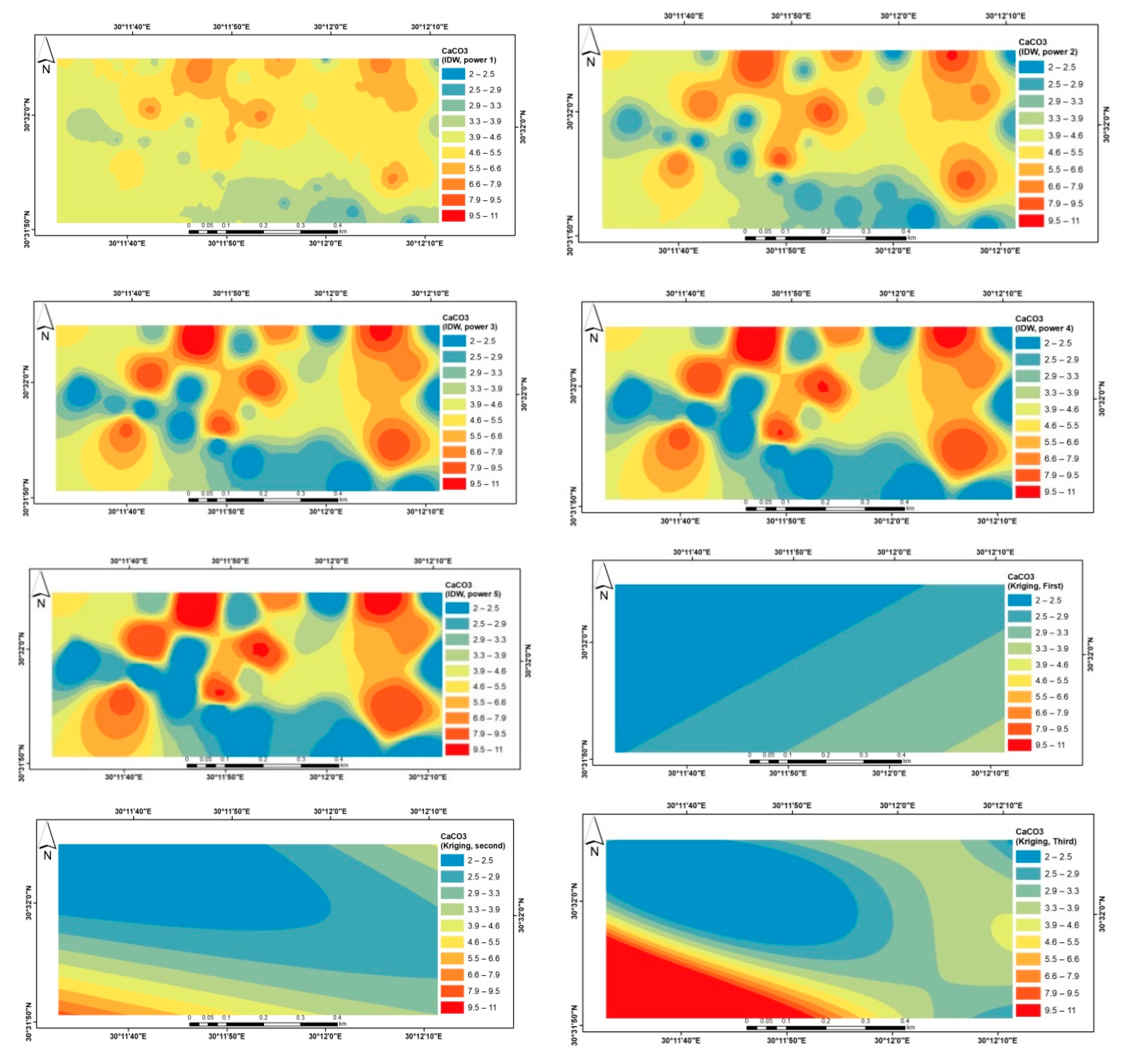
2.3. Interpolation Methods
2.4. Physical Soil Properties
2.5. Chemical Soil Properties
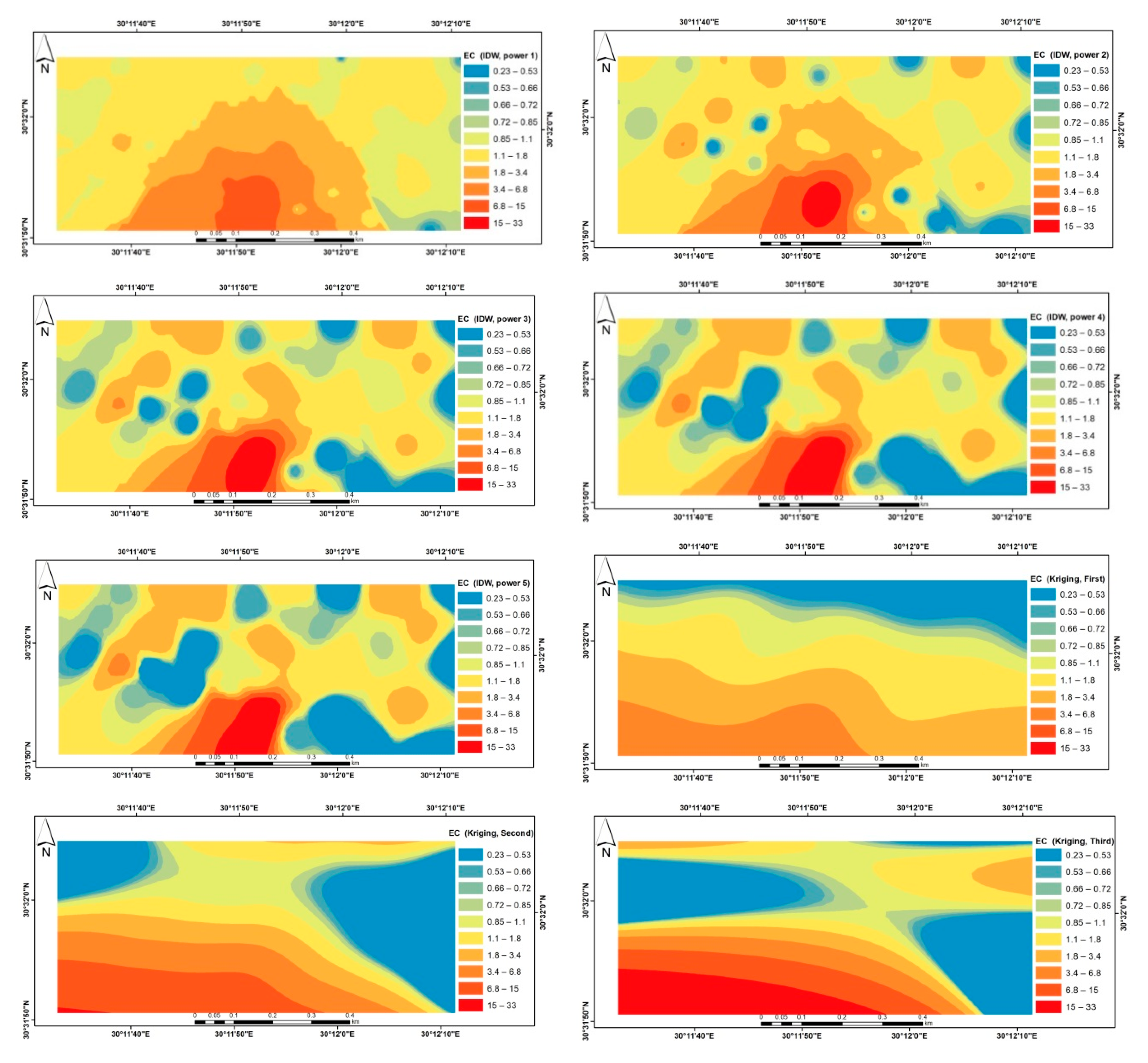
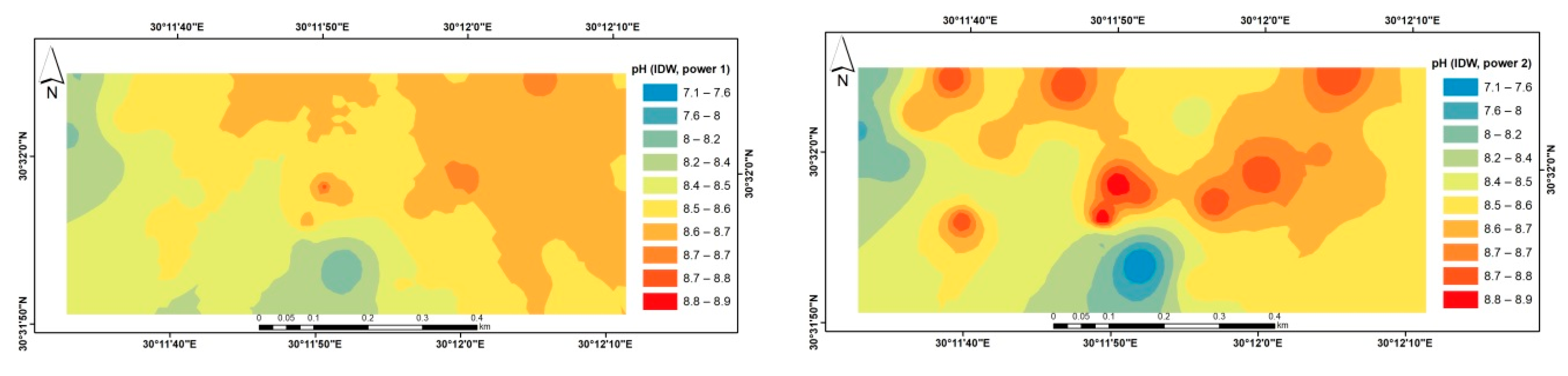
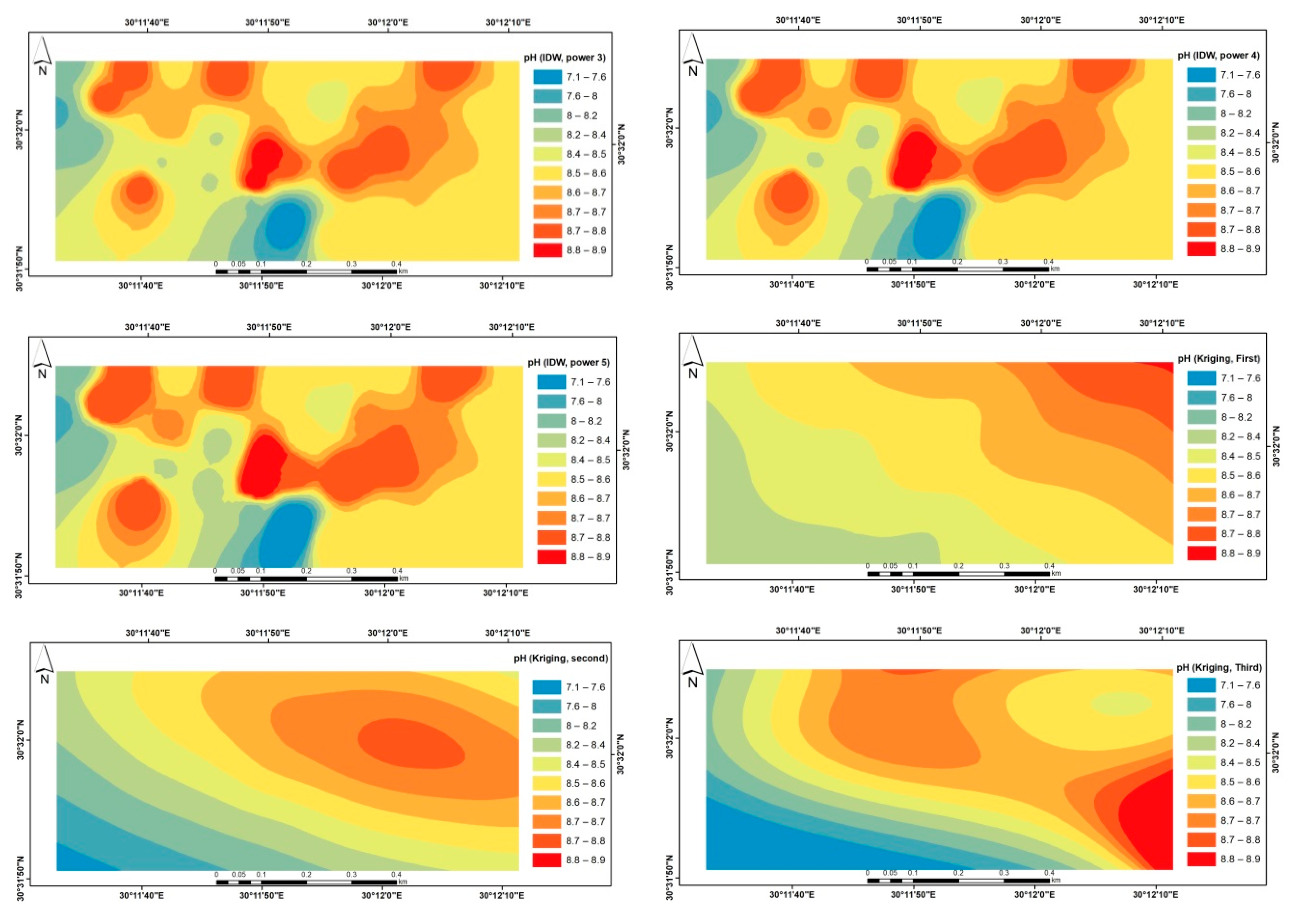
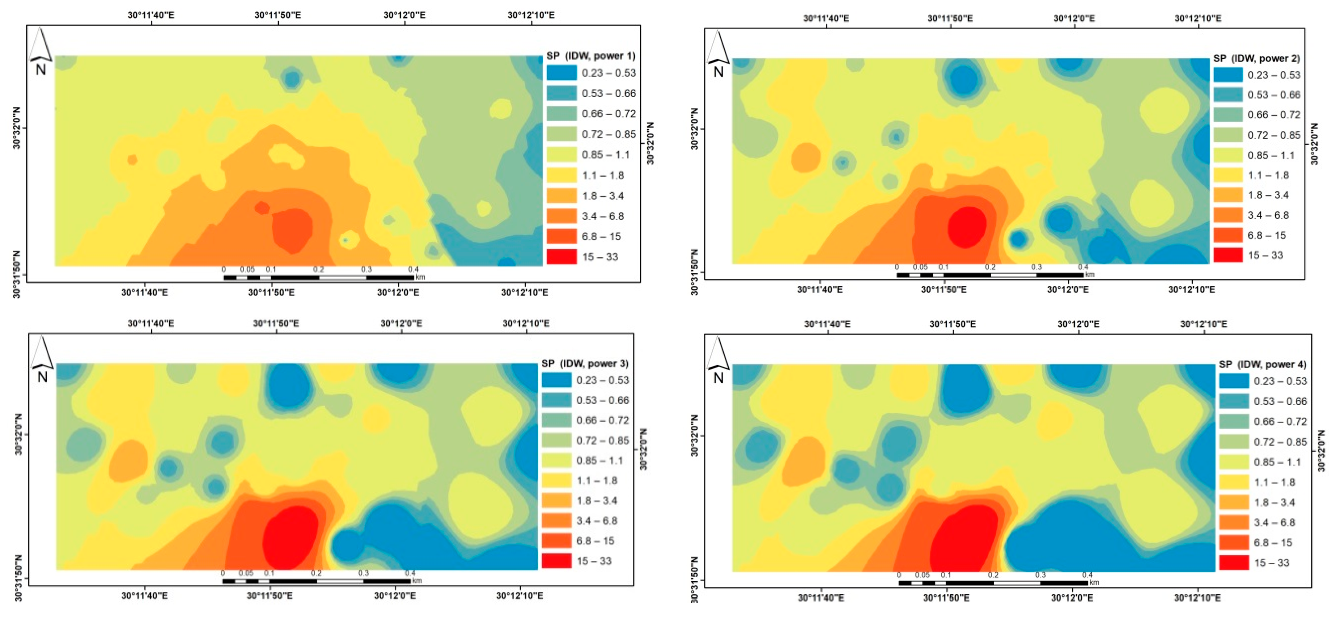
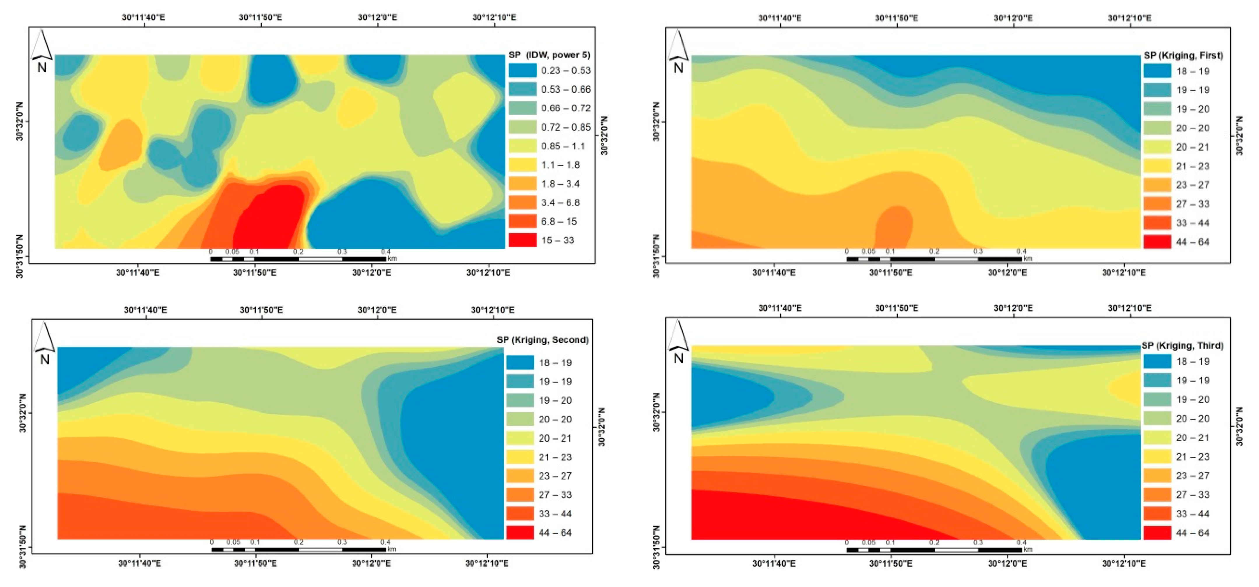
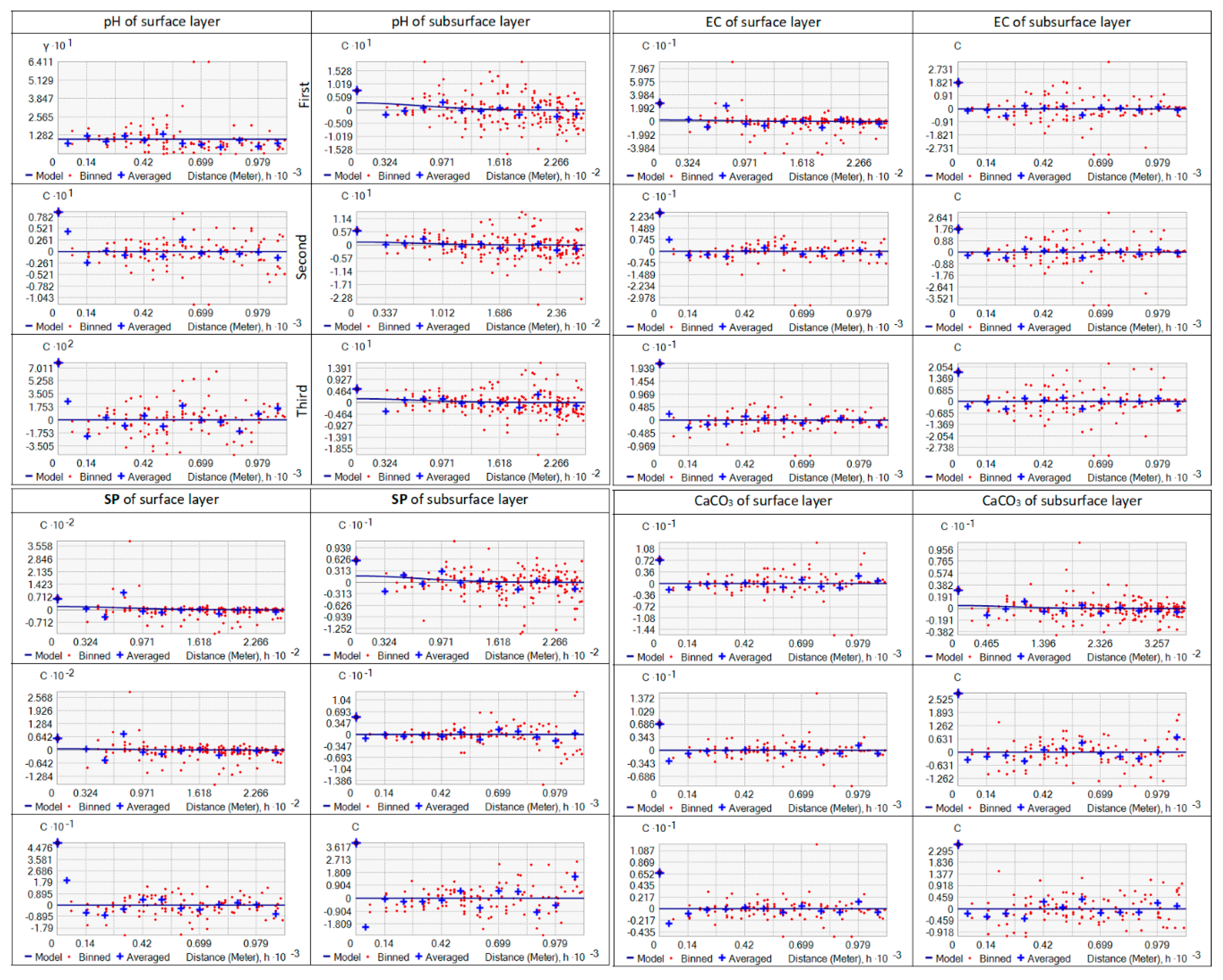
3. Results and Discussion
4. Conclusions
Author Contributions
Funding
Data Availability Statement
Conflicts of Interest
References
- Aboelsoud, H.M.; Abdelrahman, M.A.E. Rapid Field Technique for Soil Salinity Appraisal in North Nile Delta Using EM 38 through Some Empirical Relations. Int. J. Plant Soil Sci. 2017, 14, 1–9. [Google Scholar] [CrossRef]
- AbdelRahman, M.A.E.; Shalaby, A.; Aboelsoud, M.H.; Moghanm, F.S. GIS spatial model based for determining actual land degradation status in Kafr El-Sheikh Governorate, North Nile Delta. Model. Earth Syst. Environ. 2018, 4, 359–372. [Google Scholar] [CrossRef]
- Goovaerts, P. Geostatistics in soil science: State-of-the-art and perspectives. Geoderma 1999, 89, 1–45. [Google Scholar] [CrossRef]
- Zhang, S.-W.; Shen, C.-Y.; Chen, X.-Y.; Ye, H.-C.; Huang, Y.-F.; Lai, S. Spatial Interpolation of Soil Texture Using Compositional Kriging andRegression Kriging with Consideration of the Characteristics of CompositionalData and Environment Variables. J. Integr. Agric. 2013, 12, 1673–1683. [Google Scholar] [CrossRef]
- Lark, R.M. Towards soil geostatistics. Spat. Stat. 2012, 1, 92–99. [Google Scholar] [CrossRef]
- Zhang, Z.; Yu, D.; Shi, X.; Weindorf, D.C.; Sun, Y.; Wang, H.; Zhao, Y. Effects of prediction methods for detecting the temporal evolution of soil organic carbon in the Hilly Red Soil Region, China. Environ. Earth Sci. 2011, 64, 319–328. [Google Scholar] [CrossRef]
- Robinson, T.P.; Metternicht, G. Testing the performance of spatial interpolation techniques for mapping soil properties. Comput. Electron. Agric. 2006, 50, 97–108. [Google Scholar] [CrossRef]
- Sayed, R.M.; Feraidon, S.; Somayeh, D.; Mahmood, R.S.; Abass, T. Evaluating inverse distance weighting and kriging methods in estimation of some physical and chemical properties of soil in Qazvin Plain. Eurasian J. Soil Sci. 2017, 6, 327–336. [Google Scholar]
- Dripps, W.R.; Bradbury, K.R. A simple daily soil–water balance model for estimating the spatial and temporal distribution of groundwater recharge in temperate humid areas. Hydrogeol. J. 2007, 15, 433–444. [Google Scholar] [CrossRef]
- Kravchenko, A.; Bullock, D.G. A comparative study of interpolation methods for mapping soil properties. Agron. J. 1999, 91, 393–400. [Google Scholar] [CrossRef]
- Govaerts, A.; Vervoort, A. Geostatistical interpolation of soil properties in boom clay in Flanders. In GeoENV VII–Geostatistics for Environmental Applications; Springer: Berlin, Germany, 2010; pp. 219–230. [Google Scholar]
- Baskan, O.; Erpul, G.; Dengiz, O. Comparing the efficiency of ordinary kriging and cokriging to estimate the Atterberg limits spatially using some soil physical properties. Clay Miner. 2009, 44, 181–193. [Google Scholar] [CrossRef]
- Fritsch, C.; Cœurdassier, M.; Giraudoux, P.; Raoul, F.; Douay, F.; Rieffel, D.; De Vaufleury, A.; Scheifler, R. Spatially explicit analysis of metal transfer to biota: Influence of soil contamination and landscape. PLoS ONE 2011, 6, e20682. [Google Scholar] [CrossRef] [PubMed]
- Qiu, Y.; Fu, B.; Wang, J.; Chen, L. Spatiotemporal prediction of soil moisture content using multiple-linear regression in a small catchment of the Loess Plateau, China. Catena 2003, 54, 173–195. [Google Scholar] [CrossRef]
- Lesch, S.M.; Corwin, D.L. Prediction of spatial soil property information from ancillary sensor data using ordinary linear regression: Model derivations, residual assumptions and model validation tests. Geoderma 2008, 148, 130–140. [Google Scholar] [CrossRef]
- Tabari, H.; Sabziparvar, A.-A.; Ahmadi, M. Comparison of artificial neural network and multivariate linear regression methods for estimation of daily soil temperature in an arid region. Meteorol. Atmos. Phys. 2011, 110, 135–142. [Google Scholar] [CrossRef]
- Lin, G.-F.; Chen, L.-H. A spatial interpolation method based on radial basis function networks incorporating a semivariogram model. J. Hydrol. 2004, 288, 288–298. [Google Scholar] [CrossRef]
- Minasny, B.; McBratney, A.B. Spatial prediction of soil properties using EBLUP with the Matérn covariance function. Geoderma 2007, 140, 324–336. [Google Scholar] [CrossRef]
- Zhu, Q.; Lin, H.S. Comparing ordinary kriging and regression kriging for soil properties in contrasting landscapes. Pedosphere 2010, 20, 594–606. [Google Scholar] [CrossRef]
- Sun, W.; Whelan, B.M.; Minasny, B.; McBratney, A.B. Evaluation of a local regression kriging approach for mapping apparent electrical conductivity of soil (ECa) at high resolution. J. Plant Nutr. Soil Sci. 2012, 175, 212–220. [Google Scholar] [CrossRef]
- Hengl, T.; Heuvelink, G.B.M.; Rossiter, D.G. About regression-kriging: From equations to case studies. Comput. Geosci. 2007, 33, 1301–1315. [Google Scholar] [CrossRef]
- Sigua, G.C.; Hudnall, W.H. Kriging analysis of soil properties. J. Soils Sediments 2008, 8, 193. [Google Scholar] [CrossRef]
- Pandey, V.; Pandey, P.K. Spatial and temporal variability of soil moisture. Int. J. Geosci. 2010, 1, 87. [Google Scholar] [CrossRef]
- Gouri, S.B.; Pravat, K.S.; Ramkrishna, M. Comparison of GIS-based interpolation methods for spatial distribution of soil organic carbon (SOC). J. Saudi Soc. Agric. Sci. 2018, 17, 114–126. [Google Scholar]
- Lark, R.M.; Minasny, B. Classical Soil Geostatistics. In Pedometrics. Progress in Soil Science; McBratney, A., Minasny, B., Stockmann, U., Eds.; Springer: Cham, Switzeland, 2018. [Google Scholar]
- Glécio, M.S.; Jorge, D.D.; Montserrat, V.A.; Ênio, F.F.S. Using Multivariate Geostatistics to Assess Patterns of Spatial Dependence of Apparent Soil Electrical Conductivity and Selected Soil Properties. Sci. World J. 2014, 2014, 712403. [Google Scholar]
- Mehmet, Z.İ.; Elif, S. Analysis of Different Interpolation Methods for Soil Moisture Mapping Using Field Measurements and Remotely Sensed Data. Int. J. Environ. Geoinform. 2016, 3, 11–25. [Google Scholar]
- Yao, X.; Fu, B.; Lü, Y.; Sun, F.; Wang, S.; Liu, M. Comparison of four spatial interpolation methods for estimating soil moisture in a complex terrain catchment. PLoS ONE 2013, 8, e54660. [Google Scholar] [CrossRef]
- Zhang, C.; Liu, S.; Zhang, X.; Tan, K. Research on the spatial variability of soil moisture. In Proceedings of the International Conference on Computer and Computing Technologies in Agriculture, Wuyishan, China, 18–20 August 2007; pp. 285–292. [Google Scholar]
- Huaxing, B.; Xiaoyin, L.; Xin, L.; Mengxia, G.U.O.; Jun, L.I. A case study of spatial heterogeneity of soil moisture in the Loess Plateau, western China: A geostatistical approach. Int. J. Sediment Res. 2009, 24, 63–73. [Google Scholar]
- Li, J.; Heap, A.D. A review of comparative studies of spatial interpolation methods in environmental sciences: Performance and impact factors. Ecol. Inform. 2011, 6, 228–241. [Google Scholar] [CrossRef]
- Carré, F.; Girard, M.C. Quantitative mapping of soil types based on regression kriging of taxonomic distances with landform and land cover attributes. Geoderma 2002, 110, 241–263. [Google Scholar] [CrossRef]
- Stacey, K.F.; Lark, R.M.; Whitmore, A.P.; Milne, A.E. Using a process model and regression kriging to improve predictions of nitrous oxide emissions from soil. Geoderma 2006, 135, 107–117. [Google Scholar] [CrossRef]
- Li, Y. Can the spatial prediction of soil organic matter contents at various sampling scales be improved by using regression kriging with auxiliary information? Geoderma 2010, 159, 63–75. [Google Scholar] [CrossRef]
- Richards, L.A. Diagnosis and Improvement of Saline and Alkali Soils; Lippincott Williams & Wilkins: Philadelphia, PA, USA, 1954; Volume 78. [Google Scholar]
- Black, C.A., Ed.; Methods of Soil Analysis. Soil Sci. 1965, 100, 376. [Google Scholar] [CrossRef]
- Klute, A.; Page, A.L. Methods of Soil Analysis. Part 1. Physical and Mineralogical Methods; Part 2. Chemical and Microbiological Properties; American Society of Agronomy, Inc.: Madison, WI, USA, 1986. [Google Scholar]
- Page, A.L.; Miller, R.H.; Keeney, D.R. Methods of Soil Analysis; American Society of Agronomy: Madison, WI, USA, 1982. [Google Scholar]
- Piper, C. Soil and Plant Analysis; International Public Inc.: New York, NY, USA, 1950; Volume 59, p. 263. [Google Scholar]
- Ayele, G.T.; Demissie, S.S.; Jemberrie, M.A.; Jeong, J.; Hamilton, D.P. Terrain Effects on the Spatial Variability of Soil Physical and Chemical Properties. Soil Syst. 2020, 4, 1. [Google Scholar] [CrossRef]
- Liu, R.; Pan, Y.; Bao, H.; Liang, S.; Jiang, Y.; Tu, H.; Nong, J.; Huang, W. Variations in Soil Physico-Chemical Properties along Slope Position Gradient in Secondary Vegetation of the Hilly Region, Guilin, Southwest China. Sustainability 2020, 12, 1303. [Google Scholar] [CrossRef]
- Denton, O.A.; Aduramigba-Modupe, V.O.; Ojo, A.O.; Adeoyolanu, O.D.; Are, K.S.; Adelana, A.O.; Oyedele, A.O.; Adetayo, A.O.; Oke, A.O. Assessment of spatial variability and mapping of soil properties for sustainable agricultural production using geographic information system techniques (GIS). Cogent Food Agric. 2017, 3, 1279366. [Google Scholar] [CrossRef]
- Cambardella, C.A.; Karlen, D.L. Spatial analysis of soil fertility parameters. Precis. Agric. 1999, 1, 5–14. [Google Scholar] [CrossRef]
- Clark, I. Practical Geostatistics; Applied Science Publishers London: London, UK, 1979; Volume 3. [Google Scholar]
- Erşahin, S. Alluvial soil in a field, some physical and chemical properties of the spatial variability of the determination. J. Fac. Agric. 1999, 13, 34–41. [Google Scholar]
- Robertson, G.P. Geostatistics in ecology: Interpolating with known variance. Ecology 1987, 68, 744–748. [Google Scholar] [CrossRef]
- Trangmar, B.B.; Yost, R.S.; Uehara, G. Application of geostatistics to spatial studies of soil properties. Adv. Agron. 1986, 38, 45–94. [Google Scholar]
- Wang, X.; Huang, X.; Hu, J.; Zhang, Z. The Spatial Distribution Characteristics of Soil Organic Carbon and Its Effects on Topsoil under Different Karst Landforms. Int. J. Environ. Res. Public Health 2020, 17, 2889. [Google Scholar] [CrossRef]
- Zhou, W.; Han, G.; Liu, M.; Zeng, J.; Liang, B.; Liu, J.; Qu, R. Determining the Distribution and Interaction of Soil Organic Carbon, Nitrogen, pH and Texture in Soil Profiles: A Case Study in the Lancangjiang River Basin, Southwest China. Forests 2020, 11, 532. [Google Scholar] [CrossRef]
- Vieira, S.R.; Paz Gonzalez, A. Analysis of the spatial variability of crop yield and soil properties in small agricultural plots. Bragantia 2003, 62, 127–138. [Google Scholar] [CrossRef]
- Mohammad, Z.-M.; Taghizadeh-Mehrjardi, R.; Akbarzadeh, A. Evaluation of geostatistical techniques for mapping spatial distribution of soil pH, salinity and plant cover affected by environmental factors in Southern Iran. Not. Sci. Biol. 2010, 2, 92–103. [Google Scholar]
- Mirás-Avalos, J.M.; Fandiño, M.; Rey, B.J.; Dafonte, J.; Cancela, J.J. Zoning of a Newly-Planted Vineyard: Spatial Variability of Physico-Chemical Soil Properties. Soil Syst. 2020, 4, 62. [Google Scholar] [CrossRef]
- Yuzugullu, O.; Lorenz, F.; Fröhlich, P.; Liebisch, F. Understanding Fields by Remote Sensing: Soil Zoning and Property Mapping. Remote Sens. 2020, 12, 1116. [Google Scholar] [CrossRef]


| Meteorological Norms | January | February | March | April | May | June | July | August | September | October | November | December |
|---|---|---|---|---|---|---|---|---|---|---|---|---|
| Temp. mean Max °C | 19.7 | 24.5 | 26.7 | 26.1 | 30.9 | 32.8 | 33.7 | 34.3 | 32.9 | 29 | 23.1 | 20.7 |
| Temp. mean Min °C | 8.1 | 7.98 | 10.1 | 12.7 | 15.7 | 18.5 | 19.2 | 22.1 | 20.3 | 18 | 11 | 9.3 |
| Temp. average °C | 13.9 | 16.24 | 18.4 | 19.4 | 23.3 | 25.65 | 26.45 | 28.2 | 26.6 | 23.5 | 17.05 | 15 |
| Relative humidity % | 64.1 | 60.5 | 60.56 | 56 | 56.1 | 56.2 | 57.8 | 59.9 | 63.2 | 63 | 67.1 | 65.2 |
| Evaporation (mm/day) | 5.2 | 6.7 | 8.8 | 11.5 | 12.8 | 14 | 13.3 | 12.4 | 10.7 | 8.7 | 6.2 | 5.1 |
| Rain fall (mm) | 5.7 | 4.5 | 3.2 | 1.6 | 1.2 | 0.0 | 0.0 | 0.0 | 0.5 | 0.8 | 12 | 10.2 |
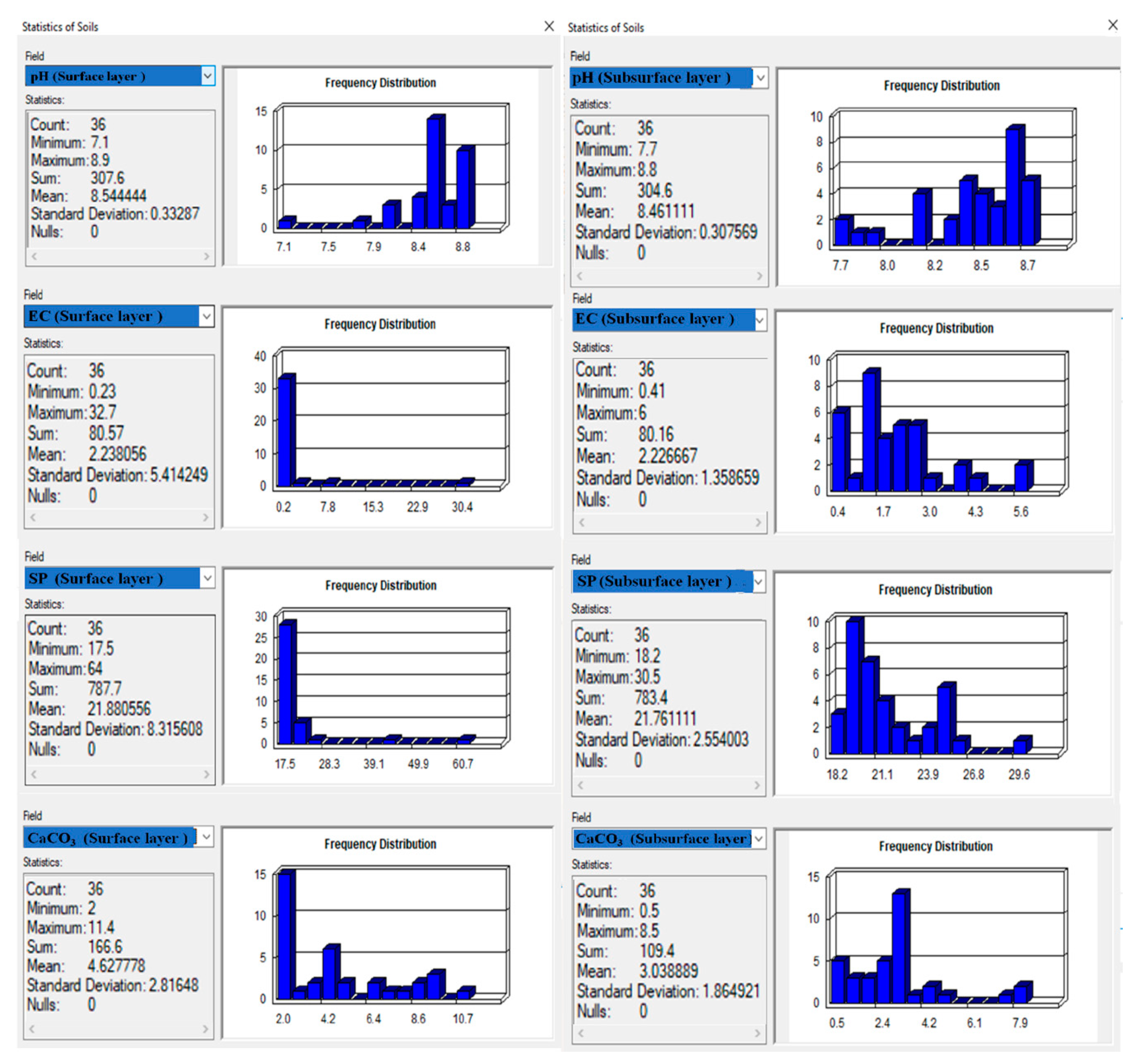
| Statistics | Surface Layer | Subsurface Layer | ||||||
|---|---|---|---|---|---|---|---|---|
| pH | EC dS/m | SP% | CaCO3 % | pH | EC dS/m | SP% | CaCO3 % | |
| Min | 7.1 | 0.2 | 17.5 | 2 | 7.7 | 0.4 | 18.2 | 0.5 |
| Max | 8.9 | 32.7 | 64 | 11.4 | 8.8 | 6 | 30.5 | 8.5 |
| Mean | 8.5 | 2.2 | 21.9 | 4.6 | 8.5 | 2.2 | 21.8 | 3 |
| Median | 8.6 | 0.8 | 20 | 4 | 8.5 | 1.9 | 21 | 3 |
| C.V% | 4 | 245.3 | 38.5 | 61.7 | 3.7 | 61.9 | 11.9 | 62.2 |
| SD | 0.3 | 5.5 | 8.4 | 2.9 | 0.3 | 1.4 | 2.6 | 1.9 |
| Skewness | −2.6 | 5.2 | 4.3 | 0.9 | −1.1 | 1.1 | 1.3 | 1.7 |
| Kurtosis | 9 | 29 | 19.5 | −0.5 | 0.6 | 1.2 | 2.2 | 2.9 |
| Statistics | Surface Layer (Meq/l) | Subsurface Layer (Meq/l) | ||||||||||
|---|---|---|---|---|---|---|---|---|---|---|---|---|
| Ca++ | Mg++ | Na+ | K+ | HCO3− | Cl− | Ca++ | Mg++ | Na+ | K+ | HCO3− | Cl− | |
| Min | 0.4 | 0.1 | 1.2 | 0.2 | 0.6 | 0.7 | 0.8 | 0.2 | 3.2 | 0.1 | 0.6 | 1.6 |
| Max | 25 | 52 | 265.4 | 1.2 | 3.9 | 254.2 | 26 | 8 | 38.6 | 0.7 | 6.5 | 31.2 |
| Mean | 2.3 | 2.1 | 17.7 | 0.4 | 1.5 | 13.6 | 4.8 | 1.8 | 14.6 | 0.4 | 1.4 | 10.2 |
| Median | 1.4 | 0.5 | 6.1 | 0.3 | 1.5 | 4.1 | 2.8 | 0.9 | 12.9 | 0.3 | 1.2 | 7.4 |
| C.V% | 186.3 | 413.3 | 250.5 | 51.1 | 36.2 | 307.9 | 115.2 | 110.1 | 55 | 50.6 | 69.8 | 72.1 |
| SD | 4.3 | 8.6 | 44.3 | 0.2 | 0.5 | 41.9 | 5.5 | 2 | 8.1 | 0.2 | 1 | 7.3 |
| Skewness | 4.7 | 5.9 | 5.3 | 1.9 | 2.4 | 5.7 | 2.4 | 1.8 | 1 | 0.7 | 4.3 | 1.4 |
| Kurtosis | 23.5 | 35 | 30 | 4.2 | 10 | 33.5 | 6.3 | 2.9 | 1.3 | −0.6 | 22.7 | 1.5 |
Publisher’s Note: MDPI stays neutral with regard to jurisdictional claims in published maps and institutional affiliations. |
© 2020 by the authors. Licensee MDPI, Basel, Switzerland. This article is an open access article distributed under the terms and conditions of the Creative Commons Attribution (CC BY) license (http://creativecommons.org/licenses/by/4.0/).
Share and Cite
AbdelRahman, M.A.E.; Zakarya, Y.M.; Metwaly, M.M.; Koubouris, G. Deciphering Soil Spatial Variability through Geostatistics and Interpolation Techniques. Sustainability 2021, 13, 194. https://doi.org/10.3390/su13010194
AbdelRahman MAE, Zakarya YM, Metwaly MM, Koubouris G. Deciphering Soil Spatial Variability through Geostatistics and Interpolation Techniques. Sustainability. 2021; 13(1):194. https://doi.org/10.3390/su13010194
Chicago/Turabian StyleAbdelRahman, Mohamed A. E., Yasser M. Zakarya, Mohamed M. Metwaly, and Georgios Koubouris. 2021. "Deciphering Soil Spatial Variability through Geostatistics and Interpolation Techniques" Sustainability 13, no. 1: 194. https://doi.org/10.3390/su13010194
APA StyleAbdelRahman, M. A. E., Zakarya, Y. M., Metwaly, M. M., & Koubouris, G. (2021). Deciphering Soil Spatial Variability through Geostatistics and Interpolation Techniques. Sustainability, 13(1), 194. https://doi.org/10.3390/su13010194