Article

On the Selection of Charging Facility Locations for EV-Based Ride-Hailing Services: A Computational Case Study

Department of Civil and Environmental Engineering, Imperial College London, London SW7 2AZ, UK
*
Author to whom correspondence should be addressed.
Sustainability 2021, 13(1), 168; https://doi.org/10.3390/su13010168
Submission received: 3 December 2020 / Revised: 17 December 2020 / Accepted: 21 December 2020 / Published: 26 December 2020

Abstract

:
The uptake of Electric Vehicles (EVs) is rapidly changing the landscape of urban mobility services. Transportation Network Companies (TNCs) have been following this trend by increasing the number of EVs in their fleets. Recently, major TNCs have explored the prospect of establishing privately owned charging facilities that will enable faster and more economic charging. Given the scale and complexity of TNC operations, such decisions need to consider both the requirements of TNCs and local planning regulations. Therefore, an optimisation approach is presented to model the placement of CSs with the objective of minimising the empty time travelled to the nearest CS for recharging as well as the installation cost. An agent based simulation model has been set in the area of Chicago to derive the recharging spots of the TNC vehicles, and in turn derive the charging demand. A mathematical formulation for the resulting optimisation problem is provided alongside a genetic algorithm that can produce solutions for large problem instances. Our results refer to a representative set of the total data for Chicago and indicate that nearly 180 CSs need to be installed to handle the demand of a TNC fleet of 3000 vehicles.

1. Introduction

Mobility as a Service (MaaS) platforms such as Demand Responsive Traffic (DRT), car-sharing and ride-sharing platforms have increasingly become popular around the world as remedial measures to reduce traffic congestion. These schemes have introduced major shifts in the interaction between travellers, transport infrastructure, and public transport schemes. Several initiatives that promote the use of MaaS schemes to reduce private usage already exist [1,2]. Their introduction has also coincided with the increasing uptake of Electric Vehicles (EVs) which are more environmentally friendly compared to vehicles with conventional combustion engines [3,4,5,6]. However, they suffer from decreased range compared to conventional vehicles. Although current research efforts are primarily focused on new battery technologies to increase their range or become affordable [7], they have not yet been developed enough to warrant widespread adoption. Charging speeds and battery capacities, which are matters of particular concern for fleet operators have been improving recently [8].
Even though there has been a continuous investment in new EV Charging Stations (CSs), the growth in the number of EVs is currently surpassing the growth in the number of charging points [9], particularly in the light of further demand. Noticeably, in 2018 only 5% of vehicle charging takes place at on-street CSs or at car parks or park & ride facilities, while the rest 95% takes place at work or at home [10]. Most ride-sharing fleet operators have plans to transition their fleets towards EVs in the near future, with many already operating a mix of conventional, hybrid and EVs. The average distance travelled by a ride-sharing EV is around 1000 miles (1600 km) per week [11], meaning that it would need to be recharged every one or two days. Adding up the time due to queue delays at CSs [12], the problem worsens. Therefore, to maintain the current level of convenience provided by MaaS platforms, the supporting charging infrastructure needs to expand considerably to sufficiently meet the demand.
Chicago is a city with high demand in ride-sharing. According to recent reports, Uber is going to invest over two billion dollars in the city of Chicago in the next decade to expand its business [13]. Furthermore, the Chicago City Council supports the transition to fully EVs and the implementation of CSs of both standard and rapid types [14]. It is estimated that up to 80,000 EVs will be adopted across the City of Chicago by 2030, meaning that around 2700 CSs will be required by then to cover the demand [15].
However, only 520 level-2 public CSs (approximately 3 h to charge with a charge current of 25-32A) and 82 level-3 CSs (approximately 30 min with a charge current up to 63A) have been deployed [16], leaving a considerable gap in the future charging demand. These calculations were made considering the C-rate (measurement of the charge and discharge current with respect to its nominal capacity).
Given this shortage, the search for an available charging location is likely to reduce the efficiency of an EV-based ride-sharing platform, and contribute to an increase in the number of overall empty vehicle-miles travelled, a commonly used metric of fleet efficiency and a proxy for contribution to congestion. Considering also that TNCs aim to transition to fully EVs by 2025 (e.g., [17]), it is evident that the number of CSs must significantly increase. Several TNCs have participated in deploying such charging facilities, and further planned to integrate EVs fleets operations with locating such CSs [18].

Our Contribution

This paper aims to find the locations of future CSs for TNC vehicles in an efficient way, and identify a number of stations that is sufficient to cover the charging demand. Having as a case study the area of Chicago, operational data of a taxi fleet are used to estimate the charging demand. Using an agent-based simulation model we derive the locations where the vehicles need recharging in the network. The candidate locations for the placement of facilities are extracted by a k-means clustering over the nodes of Chicago as extracted from Open Street Map [19]. The selected locations are obtained by solving (approximately) an optimisation problem using a Genetic Algorithm with the objective of minimising the incurred total cost (installation cost and cost for empty VMT).
The paper is organised as follows: the current literature is reviewed in Section 2. In Section 3 we describe our model and present the genetic algorithm to solve the problem. In Section 4 we present our results in a case study of the Chicago network. Finally, Section 5 concludes our study. Table 1 presents the abbreviations of the phrases used in this study.

2. Literature Review
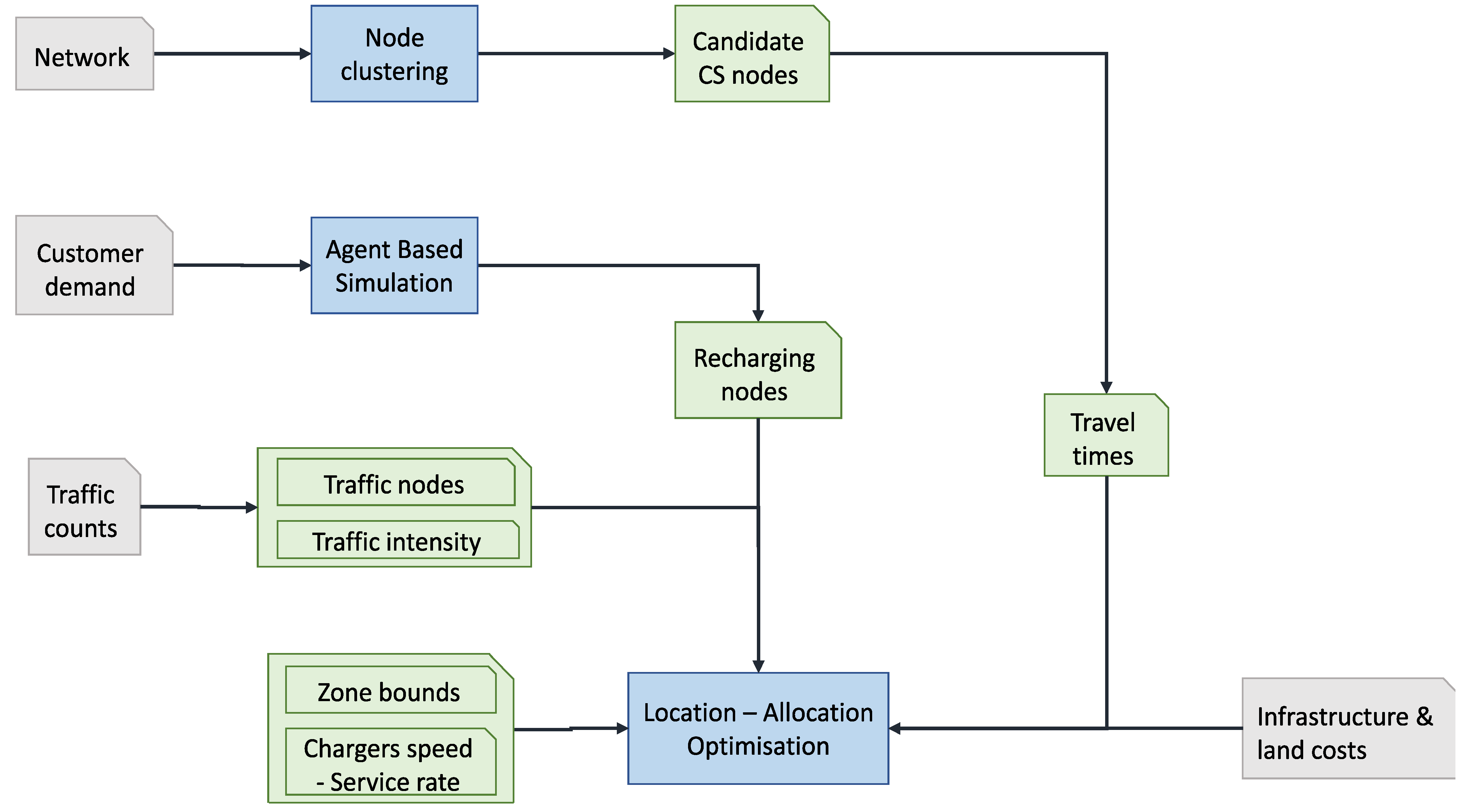
A wide range of studies have focused on variations of the charging infrastructure planning in order to assist city planners with an efficient way for the placement of resources.
Asamer et al. [20] proposed a system for the placement of a limited number of fast charging stations dedicated to ETs. The authors first identify the regions where the stations should be placed by solving an optimisation problem with the objective of maximally satisfying the charging demand under a predefined budget. A simulation of EVs in the city of Vienna using customer origin-destination trip data from radio taxi providers is performed to derive the charging demand. The exact locations within the regions are then identified by taking into account a number of environmental constraints.
Han et al. [21] proposed an optimisation model with the objective of minimising the total infrastructure cost and waiting times. GPS trajectory data from conventional taxis and battery data from EVs from Daejon were used considering the itinerary interception approach. Jung et al. [12] also considered an itinerary interception with stochastic passenger demand and proposed a bilevel optimisation-simulation model to deal with the dynamic nature of taxi itineraries and the queue delays at the stations. The upper-level problem aims to find the optimal locations of the stations and the allocation of chargers to ETs, while the lower level problem based on a simulation in the area of Seoul that uses stochastic customer demand, aims at minimising the travel times of the passengers.
Sellmair et al. [22] present an economic analysis aiming to find the optimal number of charging stations placed at taxi stands such that a trade-off between the service of ETs (mileage and earnings) and the installation cost is achieved. They present an event-based simulation in Munich using driving patterns from combustion engine taxis and proposed a heuristic to solve an optimisation problem in order to determine the optimal number of stations.
Tu et al. [23] developed a spatial-temporal demand coverage model by extracting both spatial and temporal attributes from GPS data of taxis in Shenzen. The authors aimed at the maximisation of the ET service level i.e., the distance travelled to cover the customer demand, while simultaneously minimising the total waiting time for charging.
A multi-objective optimisation framework for the deployment of ET charging infrastructure incorporating a spatial-temporal simulation model was proposed in [24] to estimate the charging demand. The charging demand is estimated according to the customer demand and the competition between the retailers. The deployment of the stations is established by taking into consideration the impact on the passengers, the drivers and the electricity retailers.
Gan et al. [25] studied the deployment of (only) fast CSs allowing a level of stochasticity, by considering elastic charging demand in the network in both the waiting time in CS queues and the covered travelled distance.
Xie et al. [26] propose a two stage method for the siting and sizing of CSs in highway networks. In the first stage the optimal locations of the CSs are extracted by the solution of a Mixed Integer Linear Program (MILP), while in the second stage the optimal sizes of the components of each CS are determined by an optimisation model.
Yang et al. [27] present a data-driven optimisation model with the objective of minimising the infrastructure cost under the constraint of charging demand satisfaction. This is achieved after deriving a trade-off between the number of charging points and the number of waiting spaces that need to be installed in the stations. The authors consider a queuing model to describe charging congestion and estimate the waiting time based on GPS trajectory data from a taxi fleet in Changsha. Due to the non-linear mixed integer nature of the queue system, the authors solve the problem approximately by transforming the formulation into an efficient Integer Linear Program (ILP).
Gacias et al. [28] study both the problem of locating charging stations (strategic level) and the charging management of an ET fleet (operational level).
Marianov et al. [29] studied probabilistic location-allocation models of maximal coverage problems and introduced an approach to constrain the waiting time at servers. Under this probabilistic approach, a constrained waiting time ILP formulation can be introduced to approximate an optimisation problem instead of a highly non-linear one where the objective minimises the waiting time of an M / M / m queuing system with a fixed number of m chargers per CS. Specifically, given input parameters α , b , the authors require that the probability of a queue of length at most b vehicles at a CS, is above a given threshold α . They later extended the model to account for variable number of chargers per CS retaining the linearity [30].
The charging demand can be addressed as point demand where the demand is aggregated in distinct places, or flow demand where the demand is represented as a flow that passes along the routes of the travellers. Table 2 sums up various features about the related works.
Opposed to previous works, an explicit distinction between on-street and off-street EV charging stations is addressed in this paper. We hereby assume that the number of on-street CSs is limited per region due to restrictions set by local authorities in order not to limit the parking spaces for the residents. Existing CSs are assumed to be on-street and can be used by either traffic or TNC vehicles, while the newly placed infrastructure can only be private property of a TNC company and therefore can only be used by its fleet.

3. Methodology

Prior to formulating the problem the following assumptions are made: (1) The battery discharges uniformly; (2) The state of charge of a vehicle’s battery after recharging at the pick-up location of a customer is 90%; (3) The threshold of the battery below which the vehicle needs recharging is set to 20%; (4) The travel time of a vehicle to go along a road is considered to be the average travel time over a day; (5) The EVs share of the total number of vehicles has been assumed to be 25% [32].

3.1. Agent Based Simulation

Operational data from Transportation Network Providers are given as input into an agent based simulation model in order to determine the recharging nodes of a fleet during the day. This simulation process has previously been used for the assignment and pricing of shared rides [33]. Figure 1 presents the flowchart of the processes in this study.
In the beginning of the simulation, the vehicles dispatch from various different locations within a predefined area. Upon receiving a trip request, the nearest available vehicle dispatches to customer’s location, assuming that there is enough battery charge to carry out the requested trip. A vehicle with fully charged battery can travel a maximum distance of 180 km. Once the battery level drops below 20% the vehicle dispatches to the nearest available CS, if no customer is served at that moment and that location is added to the set of recharging nodes. If, however, there are customers in the vehicle, it dispatches to the nearest CS once the last serving customer is dropped-off, and that drop-off location is added to the set of recharging nodes.
2

3.2. Charging Demand

The charging demand is spatially distributed and is separated into traffic demand and fleet demand. The former refers to the number of vehicles not belonging to the fleet that need recharging, and the latter refers to the number of vehicles from the TNC fleet that need recharging. At each publicly available on-street CS, the demand originates from both the TNC fleet and the traffic, while on the TNC privately owned off-street CSs, the demand originates from the TNC fleet only.

3.3. Location-Allocation Problem

Let G = ( V , E ) be the network graph with V denoting the set of nodes and E the set of links. Let C , C ^ denote respectively the set of candidate nodes and the nodes where CSs already exist. Let R denote the set of recharging nodes, i.e the locations where the fleet vehicles need to be recharged, and F denote the set of nodes where traffic is accumulated. The set of fleet vehicles that need recharging located at node r R is denoted by V r , r R and the set of traffic vehicles that need recharging located at traffic node f F is denoted by V f . Let also V R = v R V v and V F = v F V v . Table 3 presents a nomenclature of all the symbols used in this section.
The total charging demand generated at each candidate node j C is equal to the total number of vehicles assigned to it i.e., i V R V F x i j , where x i j is a binary variable indicating if vehicle i is assigned for recharging to CS located at j. We assume that traffic vehicles can be assigned only to on-street CSs, whereas fleet vehicles can be assigned to any CS.
The common goal of a TNC and the local authorities is the opening of CSs at those locations that will induce the minimum cost. TNCs are responsible for the installation of their privately owned CSs, placed either on-street or off-street, and are therefore responsible to cover all the induced costs. These include the land cost associated with the area j and the infrastructure cost β for the installation of each charger. Furthermore, if public CSs are used by TNC vehicles an annual park & charge cost p is incurred for every used charger. Therefore the total monetary cost that needs to be covered by the TNC is
M = j C j y j + β ψ j + j C ^ p i V R x i j
where y j is a binary variable indicating whether a CS is placed at location j, ω j is a binary variable indicating whether the CS at j is placed on-street (0) or off-street (1).
The empty vehicle miles travelled to recharge by the TNC fleet constitute an indirect factor of the incurred cost. Specifically, the total time needed by the TNC vehicles to reach the nearest CS, once they need recharging is
T = i V R j C C ^ t i j x i j + i V F j C ^ t i j x i j
where t i j indicates the travel time to the nearest CS j C C ^ from the location of vehicle i V R V F . Summing up all the above costs, the objective function that the TNC aims to minimise is q T + M , where q is a conversion parameter from time to monetary units.
In a similar way to [34,35] we consider CSs that act as M / M / m systems. Each CS serves the set of charging demand nodes, with the arrival rate of λ j = i V R V F x i j at node j. Assuming an exponentially distributed service rate with an average value μ j at CS j, the average waiting time at the CSs is
W = j C C ^ λ j μ j ψ j λ j
The objective function, if we consider the waiting time as an additional cost, becomes q T + M + W . Due to non-linearity of the above function we follow the approach introduced in [30] to convert the problem to an equivalent ILP. The authors showed that the waiting time of an M / M / m queuing system can be approximated by the addition of the following set of constraints:
P [ CS j has b vehicles in queue ] α , j C
These constraints state that each CS can have at most b vehicles in line with a probability of at least α , when a vehicle arrives for recharging. Marianov et al. [29] showed that the above probabilistic constraints can equivalently be written as:
i V x i j μ j ρ α j , j C ,
where ρ α j is the value of λ j / μ j for which the inequality holds with equality, assuming that m chargers are placed at CS j.
k = 0 m 1 ( m k ) m ! m b k ! 1 ρ m + b + 1 k 1 1 α
The value of ρ α j can be decreased with a manipulation of x i j (by setting many of them equal to zero). Marianov et al. [30] later relaxed this assumption to consider variable number of chargers per CS. To do so an additional set of binary variables z j r must be introduced, to indicate whether at least ψ j chargers are placed at CS j. Variable z j r has a value of 1 if at least ψ j chargers are placed at j and 0 otherwise. To ensure that z j r = 1 only if z j , r 1 = 1 , the following set of ordering constraints must hold:
z j r z j , r 1 , j C , r = 2 , , K
where K denotes the maximum number of chargers that can be placed at a CS. Using the new variables, constraints (5), for every candidate j C and every existing CS j C ^ respectively, become:
i V R x i j μ j z j 1 ρ α 1 + r = 2 K z j r ( ρ α r ρ α ( r 1 ) )
i V R V F x i j μ j z j 1 ρ α 1 + r = 2 K j z j r ( ρ α m ρ α ( r 1 ) )
ρ α j is the value of ρ for which (6) holds with equality when m j chargers are placed at CS j. The value of ρ α j can be computed for every CS j before solving the ILP using numeric root finding techniques.
Due to the restricted number of parking spaces, we have further assumed that the area of interest is initially divided into zones and that the number of on-street CSs in each zone is bounded by a specific number N z for zone z, that is provided by the local authority. Taking into account the objective function and the constraints induced by TNC and local authorities, we formulate the Charging Facility Location (CFL) problem as an Integer Quadratic Program (IQP):
min q T + M
s . t . j C ^ x i j x i j ω j = 1 , i V f , f F
j C C ^ x i j = 1 , i V r , r R
x i j y j , ( i , j ) V R × ( C C ^ ) V F × C ^
i V R x i j r = 1 K z j r , j C
i V R V F x i j K j , j C ^
z j r z j ( r 1 ) , j C , r = 2 , K
i V R x i j μ j z j 1 ρ α 1 + r = 2 K z j r ( ρ α r ρ α ( r 1 ) ) , j C
i V R V F x i j μ j ρ α 1 + r = 2 K j ( ρ α r ρ α ( r 1 ) ) , j C ^
j C n ( 1 ω j ) y j N n , n H
x i j , y j , ω j , z j r { 0 , 1 } , j C C ^ , i V R V F , r [ K ]
ψ j N , j C
where [ K ] = 1 , , K . The objective function (10) minimises the total driving time to CSs and the opening or the park & charge costs associated with CSs. Constraints (11) and (12) ensure that each traffic vehicle and each fleet vehicle respectively, that need to be recharged are each assigned to one CS. Constraint (13) forces the opening of a CS at node j, if a vehicle has been assigned to it. Constraints (14) and (15) force a candidate or an existing CS respectively at node j to have at least as many chargers as the number of vehicles assigned to it. Constraint (16) ensures the ordering of the binary variables z i.e., if CS at node j has at least r chargers installed (indicated by z j r = 1 ) then it must have first at least m 1 chargers installed (indicated by z j ( r 1 ) = 1 ). Constraints (17) and (18) bound the queue length of the candidate and existing CS at node j respectively. Constraint (19) upper bounds the number of on-street CSs at zone n. Constraints (20) force variables x i j , y j , ω j , z j r to take binary values while constraint (21) forces variable ψ j to take integer values.
We note that before solving the optimisation problem, variables y j are set to 1 and ψ j to the number of available chargers for every existing CS j C ^ . The values of variables z j r are then set according to the value of the corresponding ψ j for every existing CS j C ^ , r [ K ] .

3.4. NP-Hardness

We next consider a special case of the CFL problem with the objective consisting only of the time factor T for TNC vehicles and candidate locations and a subset of the constraints, namely (12), (13), (19). If we further omit ω j variables j C and relax equalities (12) with inequalities we derive the following problem:
min i V R j C t i j x i j
s . t . j C x i j 1 , i V r , r R
x i j y j , i V R , j C
j C n y j N n , n H
x i j , y j { 0 , 1 } , j C , i V R
which is the k-median problem known to be NP-hard [36]. As a result we get the following:
Corollary 1.
CFL is NP-hard.

3.5. Linearisation

The above IQP can be converted into an ILP [37], by introducing new variables and a set of additional constraints. The product y j ω j , j C can be linearised by introducing variable w j { 0 , 1 } and the following constraints:
w j y j , j C
w j ω j , j C
w j y j + ω j 1 , j C
Similarly we let u i j = x i j ω j , j C , i F and introduce the constraints:
u i j x i j , j C ^ , i V f , f F
u i j ω j , j C ^ , i V f , f F
u i j x i j + ω j 1 , j C ^ , i V f , f F
We also note here that ψ j can equivalently be written as m = 1 K z j m , j C C ^ .
The ILP formulation after linearisation then becomes:
min q T + M
s . t . ( 12 ) ( 18 )
( 27 ) ( 32 )
j n y j w j N n , j C
j C ^ x i j u i j = 1 , i V f , f F
x i j , y j , ω j , z j m , w j , u i j { 0 , 1 } , j C , i R F , m [ K ]

3.6. Genetic Algorithm

Since the CFL problem is NP-hard, the exact solution of the ILP (33)–(38) results in a large problem even for small instances. For this reason we solve the problem approximately using a Genetic Algorithm (GA). GA is a metaheuristic method consisting of five components: generation, evaluation, selection, crossover and mutation. The algorithm begins by generating a number of feasible solutions (population) for the problem. Each solution of the GA (chromosome) is represented by an array containing the values of the variables. Every solution is evaluated with regard to the value of its objective function.
The GA proceeds in a number of iterations (generations) to derive a solution of approximately optimal cost. Once the initial solutions have been generated, a number of the solutions are selected to be passed onto the next phases, during the selection phase. The phases that follow, crossover and mutation modify the given solutions. Specifically, crossover combines two solutions by a given probability p c while mutation alters the values of some of the variables according to a given probability p m . The purpose of randomisation aims at avoiding locally optimal solutions.
The whole process of the GA is presented in Algorithm 1. The values of the variables of each chromosome are carefully set to each chromosome in the generation phase in such a way that no constraint is violated. In the evaluation phase the value of the objective function is returned if no constraint ((34)–(38)) is violated, otherwise a very large value (indicating ) is returned. The values of the parameters for the GA can be seen in Table 4.
Algorithm 1: Genetic Algorithm (GA)
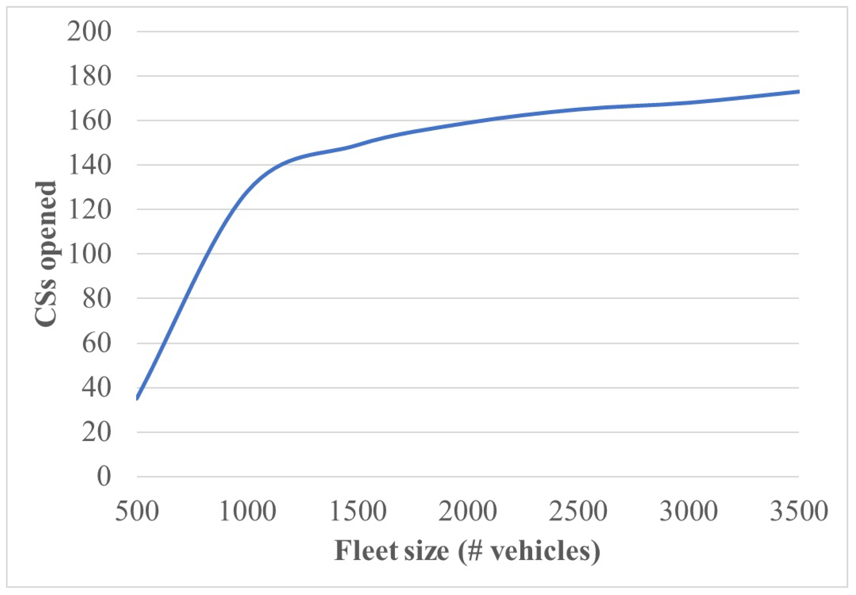
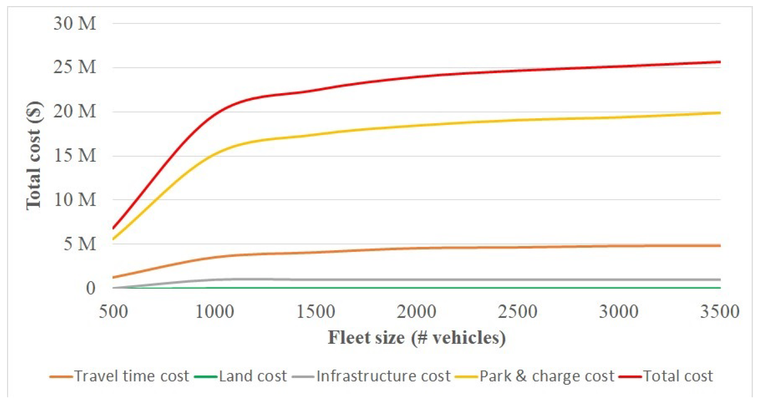
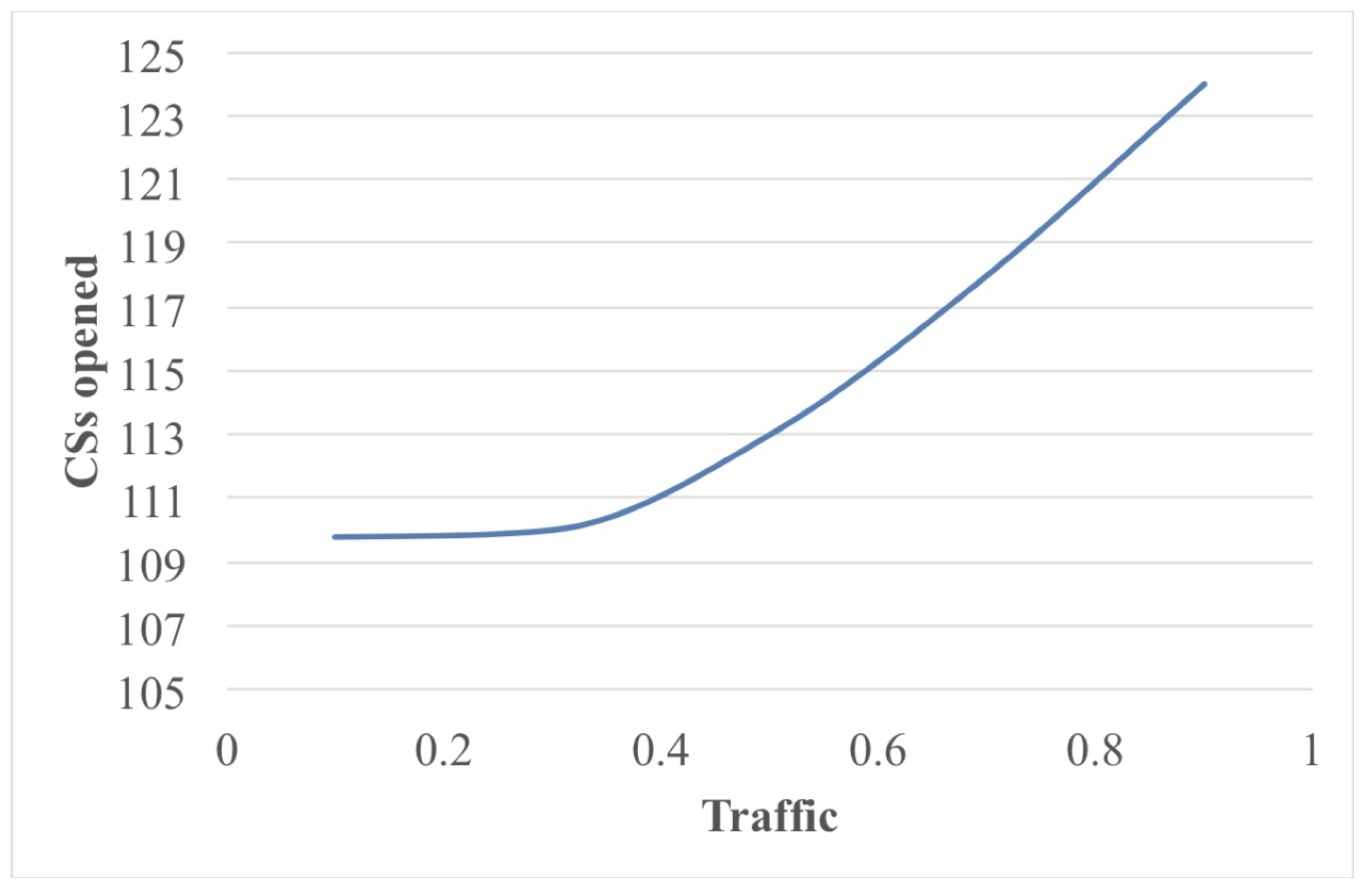
Sustainability 13 00168 i001

4. Discussion

An agent-based simulation model was implemented using C# to identify the locations where the vehicles need recharging, continuing the work on assignment and pricing of shared rides [33]. To do so, a total of 62,147 one-day taxi trips retrieved from Chicago Open Data Portal [38] have been imported into the simulation platform. Only trips with distance larger than 500 m between the pick-up and drop-off locations of the customers were considered in the simulation. The Genetic Algorithm was implemented in Python and tested on a workstation with a 16-core Intel Xeon E5-2640 v3 CPU (2.6 GHz) and 128 GB RAM.
The area of Chicago, Illinois, USA was used as a case study network consisting of 28,316 nodes and 75,758 links. The links’ average speeds were obtained from the OSMnx library [19]. The nodes that were considered as candidate locations for the placement of charging facilities, were obtained by a k-means clustering. The travel times between vehicles and candidate/existing CS locations were computed during pre-processing. The GA was implemented in DEAP [39] and was tested under fleet sizes ranging from 500 to 3500 vehicles.
Figure 2 presents a geographical distribution of the locations of existing and the suggested to be installed CSs in the area of Chicago. The numbers in the circles indicate the maximum number of available chargers in the CSs. Blue circles correspond to the locations of existing CSs, while red ones correspond to the locations suggested for the installation of new CSs.
For this study we assumed an average vehicle speed of 30 km/h throughout the whole area of Chicago and a cost per km of 0.25 $/h. With regard to the infrastructure, the installation of DC fast charger costs on average $45,000 [40,41]. Adding a maintenance cost of $1500 per year, the total cost (assuming a period of 10 years) grows to $60,000 per charger. Thus the conversion parameter of time to monetary units q is set to 0.737 . The park and charge cost is set to $9 per half hour using a DC fast charger [42]. Assuming at least 2 charges per day per vehicle the annual cost for charging in public CSs is estimated to be p = $ 6570 . Building permits were also retrieved by [38] and the land costs were computed assuming that a typical parking space is approximately 12 m 2 and a charger needs approximately 2 m 2 of space. The maximum number of chargers that can be installed per CS has been assumed to be 16. That is because the cost of opening many CSs of one charger each is much higher than the cost of opening one CS with many chargers, and therefore achieving an economy of scale. We note however, that the number of 16 chargers per CS is not strict. We did not aim to optimise this number as this is out of the scope of this work.
The nominal voltage of the batteries’ cells of the vehicle is assumed to be 360V (e.g., Nissan Leaf), the nominal capacity 40 kWh with electrolyte material of lithium-ion. The cathode material is a layer structure consisting of Lithium Nickel Cobalt Manganese Oxide, while the anode is made of graphite coated on a copper foil [43].
In Figure 3 the number of CSs that need to be opened to cover the charging demand is presented as a function of the fleet size. As can be seen from the diagram, the number of CSs that need to open rises linearly up to the size of 1000 vehicles and then it continues rising at a much smaller rate. This can be explained due to the fact that the travel time cost becomes considerable when the number of CSs is small. On the contrary, the number of CSs seems to be adequate for a larger fleet, since each CS consists up to 16 chargers (in our study).
In Figure 4 the change of the various costs is presented as a function of the fleet size. As can be observed, the total cost follows a similar trend to that of Figure 3. As explained in Section 3 the total cost is the sum of four parameters, namely the infrastructure cost, the land cost, the park & charge cost and the travel time cost, where the park & charge cost is considered only for the existing CSs.
It is evident from the diagram that the land cost is negligible. It should be noted that since each CS consists of up to 16 chargers, we claim that when there is a CS of many chargers then the infrastructure cost will be lower than that of many CSs with a single charger each, resulting in an economy of scale. As a result the infrastructure cost is very small even when the fleet sizes are large.
Furthermore, as the fleet size grows, the charging demand also grows resulting in an increase of the park & charge cost. This happens because there are not enough CSs opened in nearby areas, therefore the travel time cost remains considerable. On the other hand, if we take into consideration the diagram of Figure 3, it can be observed that at the same time the number of CSs also grows. However, after a fleet size of 1000 vehicles the increase rate slows down because there are then enough CSs in nearby areas.
In Figure 5 and Figure 6, the variation of the total cost and number of CSs that need to be opened, are studied under a fixed fleet size of 1000 TNC vehicles, with respect to the total traffic of EV vehicles on the streets.
As can be observed, the number of CSs that need to be opened presents an increase when the traffic rate exceeds 0.3, and their number needs to increase by a rate of approximately 30%. This happens because there is an adequate number of CSs up to 0.3 traffic but for traffic larger than 0.3, the needs will be satisfied with the installation of new CSs.
Furthermore, the total cost (Figure 6) seems to follow the same behaviour. This is due to the fact that TNCs try to adapt to the increasing demand by installing new CSs. As a result the expenses are mostly related to infrastructure and land costs.

5. Conclusions

In this paper we made an empirical study for the placement of charging stations dedicated to TNC EVs. We proposed a mathematical formulation for this facility location problem and solved it with a Genetic Algorithm. To the best of our knowledge, this is the first paper to explicitly distinguish between on-street and off-street facilities taking into account the restrictions that are set by local authorities with respect to the maximum number of on-street facilities per region.
Experimental results indicate that approximately 20 million dollars will need to be invested for the construction of 140 CSs, that will be needed to cover the charging demand of a TNC fleet of 1000 vehicles in the city of Chicago. The main source of expenses arises from the park & charge cost induced by the charging of the TNC vehicles in existing public CSs. Considering that the number of EVs has been increasing significantly over the last years, even more CSs will have to be constructed to cover the charging demand. Furthermore, if the fleet size consists of more than 1000 vehicles, the number of CSs does not need to be continuously proportional with the fleet size, since the charging points are adequate to cover the demand. As a result a significant amount of the investment funds can be saved. As a practical recommendation we suggest that each CS consist of many chargers in order to achieve an economy of scale.
Our suggestions for future work, include an optimisation study on the number of chargers per CSs and the study of learning methods for the calculation of the charging demand. Other solution approaches to solve the optimisation problem would include the combination of the Lagrangian relaxation method and greedy heuristic that can result in a better approximation of the objective.

Author Contributions

Conceptualization, E.A., P.A., D.A., Q.Y., P.-Y.H., M.S.; methodology, E.A., D.A., J.E.M.; software, E.A., R.K.; validation, E.A., R.K.; formal analysis, E.A.; investigation, E.A., D.A.; resources, E.A., P.A., M.S.; data curation, E.A., D.A., R.K.; writing–original draft preparation, E.A., D.A.; writing–review and editing, E.A., P.A., D.A., J.E.M., M.S.; visualization, Q.Y.; supervision, P.A., M.S.; project administration, P.A., M.S.; funding acquisition, P.A., M.S. All authors have read and agreed to the published version of the manuscript.

Funding

This research was funded by Innovate UK grant number 104271.

Institutional Review Board Statement

Not applicable.

Informed Consent Statement

Not applicable.

Data Availability Statement

The data used in this study are available at the Chicago Open Data Portal https://data.cityofchicago.org/.

Conflicts of Interest

The authors declare no conflict of interest.

References

  1. Hesketh, R.; Jones, L.; Hinrichs-Krapels, S.; Kirk, A.; Johnson, S. Air Quality Improvement Initiatives in Other Cities. 2017. Available online: https://www.kcl.ac.uk/sspp/policy-institute/publications/air-quality-improvement-initiatives-in-other-cities.pdf (accessed on 18 November 2020).
  2. Hellmann, M. Finland’s Capital Plans on Making Private-Car Ownership Obsolete in 10 Years. 2014. Available online: http://time.com/2974984/finland-helsinki-private-car-obsolete-environment-climate-change-transportation/ (accessed on 18 November 2020).
  3. Uherek, E.; Halenka, T.; Borken-Kleefeld, J.; Balkanski, Y.; Berntsen, T.; Borrego, C.; Gauss, M.; Hoor, P.; Juda-Rezler, K.; Lelieveld, J. Transport impacts on atmosphere and climate: Land transport. Atmos. Environ. 2010, 44, 4772–4816. [Google Scholar] [CrossRef]
  4. Van Mierlo, J.; Maggetto, G.; Lataire, P. Which energy source for road transport in the future? A comparison of battery, hybrid and fuel cell vehicles. Energy Convers. Manag. 2006, 47, 2748–2760. [Google Scholar] [CrossRef]
  5. Haji Akhoundzadeh, M.; Raahemifar, K.; Panchal, S.; Samadani, E.; Haghi, E.; Fraser, R.; Fowler, M. A conceptualized hydrail powertrain: A case study of the Union Pearson Express route. World Electr. Veh. J. 2019, 10, 32. [Google Scholar] [CrossRef] [Green Version]
  6. Tran, M.K.; Mevawala, A.; Panchal, S.; Raahemifar, K.; Fowler, M.; Fraser, R. Effect of integrating the hysteresis component to the equivalent circuit model of Lithium-ion battery for dynamic and non-dynamic applications. J. Energy Storage 2020, 32, 101785. [Google Scholar] [CrossRef]
  7. Kouchachvili, L.; Yaïci, W.; Entchev, E. Hybrid battery/supercapacitor energy storage system for the electric vehicles. J. Power Sources 2018, 374, 237–248. [Google Scholar] [CrossRef]
  8. Kang, B.; Ceder, G. Battery materials for ultrafast charging and discharging. Nature 2009, 458, 190. [Google Scholar] [CrossRef]
  9. London Assembly, Electric Vehicles Environment Committee, L.A. Electric Vehicles in London. 2018. Available online: https://www.london.gov.uk/about-us/london-assembly/london-assembly-publications/electric-vehicles-london-0 (accessed on 18 November 2020).
  10. Mathieu, L. Roll-Out of Public EV Charging Infrastructure in the EU. Transport & Environment, 7 September 2018. [Google Scholar]
  11. Takahashi, I. How Many Miles Do Uber and Lyft Drivers Put on Their Cars? 2018. Available online: https://ride.guru/lounge/p/how-many-miles-do-uber-and-lyft-drivers-put-on-their-cars (accessed on 18 November 2020).
  12. Jung, J.; Chow, J.Y.; Jayakrishnan, R.; Park, J.Y. Stochastic dynamic itinerary interception refueling location problem with queue delay for electric taxi charging stations. Transp. Res. Part Emerg. Technol. 2014, 40, 123–142. [Google Scholar] [CrossRef]
  13. Hodgson, C. Uber Announces $2bn Expansion of Freight Unit in Chicago. 2019. Available online: https://www.ft.com/content/6fa14cbc-d034-11e9-b018-ca4456540ea6 (accessed on 18 November 2020).
  14. Emanuel, R. Roadmap for the Future of Transportation and Mobility in Chicago: Chicago’s New Transportation and Mobility Task Force. 2019. Available online: https://www.chicago.gov/content/dam/city/depts/mayor/PDFs/21755_37_AF_MobilityReport.pdf (accessed on 18 November 2020).
  15. Ruppenthal, A. Study: Chicago Could See 80,000 Electric Cars by 2030. 2018. Available online: https://news.wttw.com/2018/02/22/study-chicago-could-see-80000-electric-cars-2030 (accessed on 18 November 2020).
  16. Chargehub. Charge Your EV in Chicago. 2019. Available online: https://chargehub.com/en/countries/united-states/illinois/chicago.html?city_id=981 (accessed on 18 November 2020).
  17. Uber UK. Uber’s Clean Air Plan to Help London Go Electric. 2018. Available online: https://www.uber.com/en-GB/newsroom/uber-helps-london-go-electric/ (accessed on 18 November 2020).
  18. Lekach, S. New Charging Network Encourages Uber and Lyft Drivers to Go Electric. 2018. Available online: https://mashable.com/2018/04/12/evgo-maven-electric-car-dedicated-charging-network/ (accessed on 18 November 2020).
  19. Boeing, G. OSMnx: New methods for acquiring, constructing, analyzing, and visualizing complex street networks. Comput. Environ. Urban Syst. 2017, 65, 126–139. [Google Scholar] [CrossRef] [Green Version]
  20. Asamer, J.; Reinthaler, M.; Ruthmair, M.; Straub, M.; Puchinger, J. Optimizing charging station locations for urban taxi providers. Transp. Res. Part Policy Pract. 2016, 85, 233–246. [Google Scholar] [CrossRef] [Green Version]
  21. Han, D.; Ahn, Y.; Park, S.; Yeo, H. Trajectory-interception based method for electric vehicle taxi charging station problem with real taxi data. Int. J. Sustain. Transp. 2016, 10, 671–682. [Google Scholar] [CrossRef]
  22. Sellmair, R.; Hamacher, T. Optimization of charging infrastructure for electric taxis. Transp. Res. Rec. 2014, 2416, 82–91. [Google Scholar] [CrossRef]
  23. Tu, W.; Li, Q.; Fang, Z.; Shaw, S.l.; Zhou, B.; Chang, X. Optimizing the locations of electric taxi charging stations: A spatial–temporal demand coverage approach. Transp. Res. Part Emerg. Technol. 2016, 65, 172–189. [Google Scholar] [CrossRef] [Green Version]
  24. Pan, A.; Zhao, T.; Yu, H.; Zhang, Y. Deploying Public Charging Stations for Electric Taxis: A Charging Demand Simulation Embedded Approach. IEEE Access 2019, 7, 17412–17424. [Google Scholar] [CrossRef]
  25. Gan, X.; Zhang, H.; Hang, G.; Qin, Z.; Jin, H. Fast-Charging Station Deployment Considering Elastic Demand. IEEE Trans. Transp. Electrif. 2020, 6, 158–169. [Google Scholar] [CrossRef]
  26. Xie, R.; Wei, W.; Khodayar, M.E.; Wang, J.; Mei, S. Planning fully renewable powered charging stations on highways: A data-driven robust optimization approach. IEEE Trans. Transp. Electrif. 2018, 4, 817–830. [Google Scholar] [CrossRef]
  27. Yang, J.; Dong, J.; Hu, L. A data-driven optimization-based approach for siting and sizing of electric taxi charging stations. Transp. Res. Part Emerg. Technol. 2017, 77, 462–477. [Google Scholar] [CrossRef] [Green Version]
  28. Gacias, B.; Meunier, F. Design and operation for an electric taxi fleet. Or Spectr. 2015, 37, 171–194. [Google Scholar] [CrossRef] [Green Version]
  29. Marianov, V.; Serra, D. Probabilistic, maximal covering location—allocation models forcongested systems. J. Reg. Sci. 1998, 38, 401–424. [Google Scholar] [CrossRef]
  30. Marianov, V.; Serra, D. Location–allocation of multiple-server service centers with constrained queues or waiting times. Ann. Oper. Res. 2002, 111, 35–50. [Google Scholar] [CrossRef]
  31. Cai, H.; Jia, X.; Chiu, A.S.; Hu, X.; Xu, M. Siting public electric vehicle charging stations in Beijing using big-data informed travel patterns of the taxi fleet. Transp. Res. Part Transp. Environ. 2014, 33, 39–46. [Google Scholar] [CrossRef] [Green Version]
  32. Statista Inc. Electric Vehicle Registrations as a Share of Total in Selected Countries Worldwide in 2018. 2019. Available online: https://www.statista.com/statistics/267162/world-plug-in-hybrid-vehicle-sales-by-region/ (accessed on 18 November 2020).
  33. Karamanis, R.; Anastasiadis, E.; Angeloudis, P.; Stettler, M. Assignment and pricing of shared rides in ride-sourcing using combinatorial double auctions. IEEE Trans. Intell. Transp. Syst. 2020, 2020, 1–12. [Google Scholar] [CrossRef]
  34. Berman, O.; Drezner, Z. The multiple server location problem. J. Oper. Res. Soc. 2007, 58, 91–99. [Google Scholar] [CrossRef]
  35. Sayarshad, H.R.; Chow, J.Y. Non-myopic relocation of idle mobility-on-demand vehicles as a dynamic location-allocation-queueing problem. Transp. Res. Part Logist. Transp. Rev. 2017, 106, 60–77. [Google Scholar] [CrossRef]
  36. Kariv, O.; Hakimi, S.L. An algorithmic approach to network location problems. I: The p-centers. SIAM J. Appl. Math. 1979, 37, 513–538. [Google Scholar] [CrossRef]
  37. Williams, H.P. Model Building in Mathematical Programming; John Wiley & Sons: Hoboken, NJ, USA, 2013. [Google Scholar]
  38. Chicago Data Portal. Chicago Open Data Web-Portal. 2019. Available online: https://data.cityofchicago.org (accessed on 18 November 2020).
  39. Fortin, F.A.; De Rainville, F.M.; Gardner, M.A.; Parizeau, M.; Gagné, C. DEAP: Evolutionary Algorithms Made Easy. J. Mach. Learn. Res. 2012, 13, 2171–2175. [Google Scholar]
  40. Cities, C. Plug-In Electric Vehicle Handbook for Public Charging Station Hosts; US Department of Energy Publication No. DOE/GO-102012-3275; US Department of Energy: Washington, DC, USA, 2012.
  41. Taxi, N.; Commission, L. Take Charge: A Roadmap to Electric New York City Taxis; New York Goverment: New York, NY, USA, 2013. Available online: http://www.nyc.gov/html/tlc/downloads/pdf/electric_taxi_task_force_report_20131231.pdf (accessed on 18 November 2020).
  42. Gorzelany, J. What It Costs to Charge an Electric Vehicle 2019. Available online: https://www.myev.com/research/ev-101/what-it-costs-to-charge-an-electric-vehicle (accessed on 18 November 2020).
  43. Miao, Y.; Hynan, P.; von Jouanne, A.; Yokochi, A. Current Li-ion battery technologies in electric vehicles and opportunities for advancements. Energies 2019, 12, 1074. [Google Scholar] [CrossRef] [Green Version]
Figure 1. Flowchart indicating the queue of processes. The processes are highlighted in blue, the input data in light grey and the processed data in green.
Sustainability 13 00168 g001
Figure 2. Map of the distribution of CSs in the area of Chicago.
Sustainability 13 00168 g002
Figure 3. Number of CSs opened in candidate locations as a function on the TNC fleet size, under an EV penetration rate of 0.2.
Sustainability 13 00168 g003
Figure 4. Cost as a function on the TNC fleet size.
Sustainability 13 00168 g004
Figure 5. Number of CSs opened in candidate locations as a function traffic of EVs for a fleet of 1000 vehicles.
Sustainability 13 00168 g005
Figure 6. Cost as a function of traffic.
Sustainability 13 00168 g006
Table 1. Abbreviations of phrases used in this study.
Abbreviations
AbbreviationsExplanation
TNCTransportation Network Companies
CSCharging Station
VMTVehicle Miles Travelled
HEVHybrid Electric Vehicle
DEAPDistributed Evolutionary Algorithms in Python
GAGenetic Algorithm
EVElectric Vehicle
ETElectric Taxi
ILPInteger Linear Program
IQPInteger Quadratic Program
CFLCharging Facility Location
MaaSMobility as a Service
DRTDemand Responsive Traffic
OSMnxOpen Street Map networkx
Table 2. Features of related papers.
Features
CitationQueue DelayCustomer DemandCharging DemandCapacityOn/Off-Street
[20]xDeterministicPointConstantUnspecified
[31]xDeterministicPointConstantOff-street
[28]xStochasticPointVariableUnspecified
[21]xDeterministicFlowVariableOff-street
[12]StochasticFlowVariableUnspecified
[24]DeterministicFlowVariableUnspecified
[22]xDeterministicPoint (taxi stands)VariableOn-street
[23]DeterministicSpatial-Temporal FlowConstantUnspecified
[27]DeterministicPointVariableUnspecified
[25]StochasticPointVariableUnspecified
[26]xStochasticPointVariableOn-street
This workDeterministicPointVariableBoth
Table 3. Nomenclature of the indices, sets, parameters and variables used in the text.
Nomenclature
IndicesDescription
iIndex of a vehicle
jIndex of a location
rIndex of a recharging node
fIndex of a traffic node
nIndex of a zone
rIndex of a charger
SetsDescription
CCandidate nodes for the placement of CS
C ^ Nodes with pre-existing CSs
RFleet recharging nodes
HZones
FTraffic nodes
V r Fleet vehicles located at recharging node r R
V f Traffic vehicles located at traffic node f F
ParametersDescription
qConversion parameter from time to monetary units
t i j Travelling time from recharging point i to nearest CS at node j
ρ α m Value of ρ = λ / μ s.t. (6) holds with equality
N n Maximum number of on-street CSs at zone n
j Land rent cost at node j
β Single charger infrastructure cost
pAnnual park & charge cost
mNumber of chargers in the queuing system
m j Number of chargers at CS j
KMaximum number of chargers at a candidate node
K j Number of chargers at existing node j
bMaximum number of vehicles in a queue
α Minimum value of the probability of b vehicles in a queue
λ j Daily arrival rate of CS at node j
μ j Daily service rate of CS at node j
VariablesDescription
x i j Assignment of vehicle i to CS at node j
y j Indicator of a CS at node j
ω j Indicator of the type of a CS off-street or on-street
z j m Indicator of at least m chargers being placed at node j
ψ j Number of chargers of CS at node j (integer)
Table 4. Values of the GA parameters.
GA Parameters
ParameterValue
Generations15
Probability of crossover0.4
Probability of mutation0.6
Population size20
Publisher’s Note: MDPI stays neutral with regard to jurisdictional claims in published maps and institutional affiliations.

