1. Introduction
It has been argued that a geographical or a spatial perspective is highly needed when it comes to public policy research [
1,
2]. This need arises in response to the diverse program designs, implementations and outcomes of public institutions. Spatial analysis of social policies can paint a picture of the wide terrain of inequality in the outcomes of public policies [
1,
2,
3].
The present study applies spatial analyses for the safety-net program Temporary Assistance for Needy Families (TANF). TANF is a mix of federal and state funds. The program not only provides cash assistance to needy families with children but also work support. Work support includes child-care, education, job training and transportation [
4]. Over the years, the proportion of TANF funds devoted to cash assistance has decreased drastically because many states opted to spend much of their monies on work support as well as other supportive services. The share of cash assistance out of total budget varies greatly by states. In 2013, for example, cash assistance varied from a minimum of 7% of total budget in Illinois to a maximum of 52% of total budget in Maine [
4].
The present study examines the TANF program in each state and its policies during the 2008 recession, often referred to as the Great Recession. During the recession, many American families with children relied on TANF for cash assistance as well as other benefits, as for example, Supplemental Nutrition Assistance Program (SNAP), previously known as food stamps [
5].
The application of spatial analyses to the TANF program has several merits. First, we shed light on horizontal equity issues geographically associated with the cash assistance aspects of the TANF program. In other words, the extent to which similarly situated families are treated in the same fashion in different states is better understood through spatial analysis. Second, we see how states’ TANF policies bear resemblance to surrounding or neighboring states’ policies. Some earlier evidence reveals that individual states’ policy makers pay attention to their neighbors’ policies in order to avoid becoming too attractive to poor families with children from surrounding states. Sometimes states avoid becoming “welfare magnets” by making their public assistance program less or about as attractive than the ones in neighboring states [
6,
7,
8,
9]. Finally, applying spatial analysis for the TANF program supports the overarching goal of engaging in evidence-based policy making. Policy makers and academics alike want policy research and spatial analyses to be at the heart of policy making [
3]. While such efforts are found to a lesser degree in social policy, in the field of regional science researchers often inform policy makers of the extent to which regions or urban areas share economic or social problems [
10,
11].
For our analyses, we use states as the unit of analysis and make regional comparisons among multistate regions. In the U.S., on social matters such as education, crime and cash assistance for poor families with children, many states’ decisions are protected from the power of the federal government. While the federal government assists states with some of the costs associated with the TANF program, the direct financial cash assistance for the nation’s poorest families with children primarily resides in each state’s government [
12]. In turn, the states are the units of analysis in this study. The Maintenance of Effort (MOE) is a federal requirement that states must spend at least a specified amount of state funds for TANF benefits and services for members of needy families with children each year [
5].
Since 1996, the federal government granted state governments the flexibility to design and administer their own TANF programs [
13]. Both need standards and maximum payments families receive depend on which state these families reside. Each state defines the amount of income essential for basic consumption (need standard) and the part of this standard paid to families (payment standard) [
12]. As of 2018, benefit levels of across the states have left families below half of the federal poverty line in almost all of states [
14].
Rather than conducting our study during the national recession of 2008, we examine the recession of individual states, which often lasted longer than the national recession. This is consistent with some earlier findings, which revealed that, in fact, there were 51 different recessions [
5,
15,
16]. In most states, the unemployment rate began rising before 2007 and kept on increasing in many states until 2011. While the unemployment rates in the states were increasing, the TANF caseloads were also increasing in response [
5,
15,
16].
Our study not only examines individual states’ recessions but also examines regional variations in the recession. The evidence is strong that select regions in the country and in turn some neighboring states within the same regions experienced similar economic downturns during the 2008 recession [
5,
15,
16]. For example, the West region of the U.S. witnessed a worse economic downturn than the other regions. A limited amount of research has been devoted to examining the extent to which states’ TANF caseloads changed in response to the 2008 recession. For the present study, we develop a relative index of TANF responsiveness to the 2008 recession that accounts for each state’s labor market performance. Thereafter, we apply an Exploratory Spatial Data Analysis (ESDA) method, which is a geographical or spatial approach to analyzing the presence of similarities or differences between neighboring states with regards to their economic dimensions, TANF responsiveness index score and TANF policies. Earlier research shows that these dimensions are good predictors of TANF enrollment [
15]. To our knowledge, very few studies were devoted to analyzing the spatial nature of these selected dimensions during the 2008 recession.
Prior to applying a spatial analytic approach, we review existing evidence about states’ economic conditions, TANF policies and TANF responsiveness to the 2008 recession.
2. Background
The research about the spatial nature of the TANF program, its policies or caseloads is in short supply. In turn, we also review related research. The review of related research examines TANF response to labor market performance during the 2008 recession on a national and state levels as well as TANF policy choices that affected TANF enrollment during the recession.
2.1. TANF Response to Great Recession
All else constant, it is reasonable to assume that TANF caseloads would increase when the unemployment rate increases since, more families would have applied for assistance and fewer families would have been able to leave the system for jobs. Most previous studies of TANF caseload in response to the 2008 economic downturn did not conduct multivariate analysis that explains changes in the TANF caseload to labor market performance by controlling for other factors than the economy [
5,
17]. Most studies were mainly concerned with examining national TANF caseload growth rate during the 2008 official national recession. Those descriptive studies concluded that in comparison to safety nets such as Unemployment Insurance, TANF grew quite modestly between December 2007 to June 2009 [
17,
18,
19]. Most researchers examined the response of TANF to the 2008 recession by computing the nationwide TANF upsurge between December 2007 and June 2009, officially defined as the Great Recession by the National Bureau of Economic Research (NBER). Their findings showed that the national TANF caseload increased by 6.8 percent [
5].
In contrast, other researchers computed the increase of the unemployment rate in each state, showing that in the majority of states (36) the unemployment rate increased from 2006 to 2011 [
5,
15,
16]. In Alaska, the unemployment rate increased by only 39%, whereas in Utah, the corresponding figure was 245 percent. Taken together, on average, the unemployment rate increase was 133 percent. Thirty-six states experienced an increase in unemployment of over 100 percent [
5].
Using the increase in unemployment rate in each state, some findings show that the TANF caseload increased by 30% rather than 6.8% when measured on a national level. Furthermore, a lag of 12 months was found between the rise in unemployment rate in a state and the rise of TANF in response [
5]. Other studies revealed that there was a lag of seven months in TANF response to the official recession [
17].
Taken together, earlier descriptive studies, whether conducted on a national or state level, captured the increases in TANF caseloads without simultaneously capturing the relative growth in unemployment rate in a state. Clearly, when unemployment rate increase in a state is small relatively to other states, it would be expected that TANF enrollment would be small in response. Thus, on a state-level, the responsiveness of TANF to the Great Recession of 2008 is best understood when TANF growth rate during a state’s own recession is calculated relative to other states’ growth of their TANF caseloads as well as the states’ own growth of unemployment relative to other states’ unemployment growth. With such calculations in hand, it is possible to accurately make comparisons for TANF responsiveness to the recession among states and to discern spatial patterns.
Recognizing that other factors play a role in shaping TANF caseloads, multivariate studies that were conducted about the 2008 recession consistently showed the important role that unemployment rate plays in shaping the size of the TANF caseloads [
20]. In each multivariate study, the impact of the unemployment rate on TANF caseload was sizable and statistically significant. For example, one study suggested that, all else constant, for 1% increase in the unemployment rate, in a typical state, TANF increased from about 29,190 TANF to 33,920 cases [
15].
The present study compares relative growth rates of TANF responsiveness to labor market conditions between states. Therefore, it develops an index that captures such responsiveness and allows for comparisons of responsiveness between the states. Using this index, we apply spatial analysis to compare neighboring states for their responsiveness.
2.2. TANF Policy Choices: Earlier Findings
Since the passage of welfare reform in 1996, the TANF system has adopted very strict policies nationwide. Federal guidelines stipulate that after five years of receiving cash assistance during a lifetime, TANF recipients are no longer eligible for such assistance. In some states, however, recipients can continue receiving cash assistance, but only with state funds. Moreover, in some states, there is a “sit out” requirement for a period of time before recipients are allowed to receive further assistance. The sit out requirements exist in a few states and vary by state [
15]. Federal guidelines further stipulate that, unless exempt, TANF recipients, need to participate in employment-related activities for a minimum of 30 h per week. Taken together, states can implement stricter requirements than the ones imposed by the federal government. In order to receive any federal funds, however, states must comply with minimum federal regulations of 30 h of work and 60-month lifetime limits. States impose sanctions when recipients violate work requirements or other requirements which vary in severity from state to state [
15,
20].
Some evidence shows that states or local implementation of stringent TANF policies cannot be explained by worsening economic conditions. Some findings suggest that administrative practices such as sanctioning are better explained by the political rather than economic climate. In some instances, TANF administrative practices deter some families from applying or staying on the rolls [
13,
21,
22]
The creation of the TANF program with stringent policies resulted in much discontent and deliberation between policy makers about the potential consequences of granting the states and local authorities so much flexibility in the design and implementation of their TANF programs. Some argued that such an arrangement would result in stringent administrative practices on a local level, which would deter families from applying for aid or from continuing receiving aid [
13]. Others argued that some families would migrate to more generous states and that states would engage in a race to the bottom in which they would make their program less attractive than their neighbors in order to discourage poor families from moving to their states [
23].
Some researchers maintain that the modest increase of 6.8 percent of the national TANF caseload during the Great Recession was primarily due to strict welfare reform policies such as the lifetime limits or sanctions that accompanied the 1996 reforms [
17]. Some evidence shows that since the passage of welfare reform legislation, the number of families on the TANF caseload had declined substantially, from about 4.8 million families in 1995 to about 1.6 million families at the beginning of the official Great Recession of 2008. The share of the poor who received TANF cash assistance after 1996 dropped considerably [
5]. On a national level, one study evaluated the impact of several 1996 provisions on the national TANF caseload during the official 2008 recession [
20]. Using administrative data from 1980 to 2009, the findings suggest that in the absence of the 1996 lifetime limits, work mandates and sanctions, there would have been more families with children enrolled in the program nationwide [
20].
A later study considered state-to-state variations in policies and economies and how these shaped enrollments during the 2008 recession [
15]. The study found that, during the 2008 recession, under the presence of temporary or lifetime time limits, cuts in benefit levels, or the multiple severe mandates, the TANF caseload did not grow as much as it would have in the absence of these policies [
15].
2.3. Geographic Analyses of TANF Policies
Dating back to the 1990s, several researchers argued that, in order to control program costs, state or local governments engage in a “race to the bottom”, which means that they modify their program features such as benefit levels or sanctioning policies so that their programs are more stringent or less attractive than their neighbors. Such program changes are done in the hopes that fewer poor families with children migrate to their states [
7,
8,
24] Some evidence shows that the fears of migration have led several states’ policy makers to cut their benefits levels [
25,
26]. While these fears exist, the evidence is mixed regarding the extent that families actually migrate to neighboring states in order to increase their public assistance benefits [
6]. An early study in the 2000s applied spatial, temporal, and spatial–temporal approaches in order to explore the extent to which states and their neighbors changed their TANF cash benefit levels relative to their neighbors [
6]. Using a tree-based regression approach, the country was divided into regions where benefit levels are relatively homogeneous within each region yet quite different between the regions. The findings suggested that both high-benefit and low-benefit states paid attention to the generosity in benefit levels of their neighbors [
6].
Confirming earlier results, a recent study conducted during the 2008 recession tested the “race to the bottom” theory by investigating whether states’ TANF eligibility requirements and the portion of the state budget devoted to TANF expenditures competed with those of neighboring states [
9]. The findings show that state policy makers do not change their TANF policies when a greater percentage of their state population becomes poorer. Rather, TANF’s budget and expenditures are affected by the budget choices of their neighboring states. Their findings showed that if neighboring states increase their spending for TANF by one unit, the subject state decreases their spending by 0.49% unit per capita. These findings apply to some states more than others [
9].
Taken together, the studies exploring geographic patterns of TANF policies or TANF responsiveness to the economy during recessions are in very short supply.
3. Objectives, Questions and Sample
Our main objective is to gain an in-depth understanding of spatial distribution patterns of the economies, varying TANF policies such as cash benefit levels and TANF caseload changes in response to the recession in the contiguous jurisdictions and District of Columbia (D.C.). during each of their 2008 recessions. We applied spatial analyses to selected variables because they were found to be good predictors of TANF enrollment in earlier research.
In turn, we ask the following research questions: (1) How did unemployment rate and TANF growth rates vary across states during their own 2008 recessions? (2) How did selected TANF policy choices such as benefit levels or sanctions vary across states when TANF was at its peak in each state’s recession? (3) How responsive was TANF to the 2008 recession in each state? To answer this last question, we developed an index that allowed us to compare TANF responsiveness in states with different labor market performance.
We used an Exploratory Spatial Data Analysis (ESDA) approach in order to identify the spatial regimes including clusters and outliers, as described in the method section of this paper. Some of the questions asked when using the tool were as follows: (1) Were there any spatial associations of unemployment growth, TANF growth or TANF responsiveness at the state level during the 2008 recession of each state? (2) Were there spatial associations of TANF maximum aid (payment levels) or other policy choices during the 2008 recession of each state? (3) Was there global spatial autocorrelation and local autocorrelation or was there statistical significance with each dimension? We applied the Moran I statistics to test global spatial autocorrelation and LISA (Local Indicator of Spatial Association) to test the presence of any spatial associations at state level.
We analyzed all contiguous jurisdictions including D.C. when mapping unemployment rate. Throughout the study we use the U.S. Census definitions of Regions. There are four census regions in the U.S.—West, Midwest, South and Northeast—defined by U.S. Census. Three Census Regions (West, Midwest, and Northeast) are made up of two census divisions, while South Census Region is composed of three census divisions. In total, there are nine census divisions and each division is decomposed of multiple states. (Map of Census Regions and Divisions can be found in the U.S. Census link,
https://www.census.gov/geographies/reference-maps/2010/geo/2010-census-regions-and-divisions-of-the-united-states.html.)
Of 13 states in the West Region, Alaska and Hawaii were dropped from the analyses because these are not contiguous to other states in the present study. The 11 West region states excluding Alaska and Hawaii witnessed a relatively more severe economic downturn than states in other regions. As further explained in the paper, when analyzing TANF caseload changes, we also excluded four states because these states witnessed a decrease in their TANF enrollment while their unemployment rate was increasing. These states are Georgia (GA), Indiana (IN), North Dakota (ND) and Rhode Island (RI). The downward trend in their TANF enrollment existed prior to the 2008 recession in these states. The observation period for the present study was from January 2005 until December 2013.
4. Data and Variable Calculations
The study uses multiple methods in order to understand spatial patterns and associations of regional and states’ TANF policies and of TANF responsiveness. Prior to applying an exploratory spatial method, we calculated the unemployment growth rate, TANF growth rate and TANF benefit levels during each state’s recession as discussed below.
4.1. Using State Level Data
As discussed earlier, while the federal government requires that states use some of their own funds for cash assistance (MOE), TANF eligibility and payment decisions as well as other policy decisions are the responsibilities of the states. Consistent with some earlier research that examined TANF caseload change as a response to changes in unemployment rate or to changes in policy choices on a state level, we used state-level data for our various analyses [
5,
15,
16]. As evidence also demonstrates, states’ economies, often correlated with changes in TANF caseloads, varied substantially during the 2008 economic downturn in both duration and in depth [
5,
15,
16]. Therefore, we also use states’ TANF unemployment rate data in order to examine spatial variations in the economy, as well other variables which explain changes in TANF caseloads.
4.2. The Unemployment Growth Rate
The unemployment rate is an important measure, but not the only measure, of a state’s economic health. In order to determine increases in the unemployment rate in each contiguous jurisdiction and D.C. during the 2008 economic downturn, we first retrieved monthly unemployment rate data for January 2005 to December 2013 from the Bureau of Labor Statistics’ (BLS) seasonally adjusted statewide unemployment rate.
Thereafter, we computed changes in the unemployment rate (seasonally adjusted) from each state’s unemployment rate from the base month to its peak month. We set the base month to be the month with the lowest unemployment rate before it began to rise substantially to its peak. The peak month was the month with the highest unemployment rate between December 2006 and December 2013. The peak months of the unemployment rate varied substantially from state to state. For example, whereas the peak month in Alabama was 12/09, the one in Colorado was 11/10.
Our findings revealed that the unemployment rate began rising in 35 contiguous jurisdictions before the official start date of the Great Recession. In five of those states, unemployment rate started to increase almost a year before the start of the official recession date, December 2007. The unemployment rate continued to rise in 48 contiguous jurisdictions after the end of the national recession in 2009.
In comparing the rise in unemployment rate between regions, the western region witnessed a relatively larger increase in its unemployment rate than other regions. Nine out of 11 western states witnessed above-national-average rise in unemployment rate. Washington (WA) and New Mexico were the only two states in the western region that experienced slower growth of unemployment rate than the national average.
4.3. TANF Caseload Growth Rate
States with larger increases in their unemployment rates during the 2008 recession would be expected to have relatively larger increases in the number of families participating in the program in response. We received TANF caseload data from the Center on Budget and Policy Priorities (CBPP). The center received TANF data directly from each state.
In order to smooth out the seasonality of the TANF caseload, we applied a 12-month moving average to each state’s TANF caseload. Such an approach is consistent with the approach used for the seasonally adjusted unemployment rate.
For each state, we calculated TANF caseload growth rate from its trough to its peak month. In each of the selected states, the caseload started to rise after the unemployment rate began to rise significantly. The TANF caseload often peaked after or right before the unemployment rate peaked. With the exclusion of the four states mentioned earlier, our findings reveal that all other contiguous jurisdictions and D.C. experienced an increase in the number of program participants. The dates for TANF peak varied, whereas in California the TANF peak date was 06/11, in Alabama the TANF peak date was 12/10.
Calculations show that Utah and Nevada had the greatest growth in unemployment rates and that their growth in their TANF caseloads was greater than the national average growth. In contrast, whereas Arizona witnessed above average increases in its unemployment rate, its TANF caseload grew at below average rate. Some states in the nonwestern region experienced below-average unemployment rate as well as below-average growth in the TANF caseload.
4.4. States’ TANF Policy Choices: Maximum Aid and Other Policy Choices
We selected a TANF maximum payment level for a family of three with zero income as one of the policy choices because this variable has repeatedly shown to be a good predictor of TANF enrollment [
15]. As of July 1, 2018, every state’s TANF benefit level for a family of three with no other cash income was at or below 60 percent of the poverty line, measured by the Department of Health and Human Services’ (HHS) 2018 poverty guidelines. Most states’ benefits were below 30 percent of the poverty line [
14]. In July 2018, Alabama’s benefit level for a family of three with no other income was
$215 (12.4% of the federal poverty level). Corresponding figures for New Hampshire and Connecticut were 60% and 40.3%, respectively. In some rare instances, some states decide whether benefits levels should vary by region within a state. For example, California has two regional benefits. The first region consists of the most populous counties. In Connecticut, one region consists of the highest-cost counties. Levels of payments for regions in a state are set by the state and not county or state-level region [
14]. We selected the highest payment level in a state. In real terms, in the majority of states, TANF cash benefits are worth at least 30 percent less today than they were in 1996 [
14].
We took the value of at TANF maximum aid at the date of peak month of TANF caseload, which varied from state to state. This variable was deflated by the consumer price index provided by BLS and recalculated in constant 2007 U.S. dollar terms. Cash assistance benefit levels were provided by US Department of Health and Human Services, Administration for Children and Families.
Table 1 shows states’ other policy choices aside from maximum payment level during their recessions. Typically, these policies do not vary across a single state. These variables’ sources were found in the Urban Institute’s welfare rules data book for several years around the states’ 2008 recession. For an example, see source for 2010 [
27]. We coded each policy choice as a dummy variable (1 = present and 0 = absent). For example, severe lifetime limits (less than five years) was coded as 1 when it was present and 0 when it was absent. We coded the policy choice at the date of each state’s TANF caseload peak.
We started by selecting an important policy choice entitled “severe lifetime limits or temporary time limits”. When states opted to require time limits that were temporary or less than the five years mandated by the federal government, we assigned a code equal to 1, otherwise 0 was assigned. The second policy choice was “severe work requirements”. As mentioned earlier, the federal requirements are that, with some exceptions, heads of household in the TANF program engage in work related activities (e.g., on job training or paid job) for a maximum 30 h per week. We assigned a code of 1 when a single head of household was required to work more than 30 h per week, 0 otherwise. The next policy variable is “severe sanctions”. We assigned a 1 when a state cuts an entire family’s benefits in response to a violation or when a case was closed for at least six months and the family had to reapply for assistance.
In some states, diversion payments and mandatory job search are applied at the point of entry to the program. As of July 2010, 75% of states offered diversion payments as a lump-sum cash payment instead of a long-term monthly payment [
27]. When states had diversion payments or mandatory job search at entry, a code of 1 was assigned and 0 otherwise.
Table 1 shows which states had severe policies at their TANF caseload peak during the state’s 2008 recession. Of the contiguous western states, California, Idaho and Nevada had two severe policies at their TANF’s caseload peak month during their 2008 recession. Yet, despite the presence of these policies, the three states’ TANF caseloads grew substantially during the recession. The remainder of the western contiguous states did not have more than one severe policy. Interestingly, in
Table 1, there are no severe policies in place at Arizona’s TANF peak. However, it should be noted that Arizona’s TANF peak occurred in December of 2009 and the state became more restrictive over time, implementing more severe policies. For instance, in 2010, Arizona changed its lifetime limits from 60 months to 36 months, and further down to 24 months in 2011. Additionally, at its TANF peak, Arizona’s maximum aid amount for a family of three was the lowest outside of the southern region. After the TANF peak in Arizona in 2009, unemployment rate had continued to rise another four months until March 2010 [
15].
4.5. TANF Responsiveness Index
As discussed earlier, evidence demonstrates that TANF caseload size is not solely a function of the labor market performance. Unemployment rate, however, is a strong predictor of TANF caseload size [
15,
20]. In order to compare relative TANF caseload growth relative to labor market performance, we created the following TANF responsiveness index:
where,
As evidenced by the equation, for each state’s recession, we are examining what happened to TANF’s caseload growth with respect to the average TANF caseload growth in all sampled states relative to each state’s growth in the number of unemployed with respect to the average growth in the number of unemployed among all the sampled states. The time period of responsiveness ratio varies by state because individual states’ recessions vary between the 45 contiguous jurisdictions. For example, assume the responsiveness rate for a state is two. This means the growth of a state’s TANF caseload with respect to the average growth of all selected states’ TANF caseload was 200% of the growth of the state’s TANF number of unemployed with respect to the average state’s growth of number of unemployed. This means that the state’s caseload is responding at twice the rate of the average of the individual state’s caseload. On the other hand, assume a state’s responsiveness is a half. This means that the growth of that state’s TANF caseload with respect to the average growth of the selected states’ TANF caseload was 50% of the growth of the state’s TANF number of unemployed with respect to the average state’s growth of number of unemployed.
It should be noted that for this calculation, we used the seasonally adjusted number of unemployed rather than the unemployment rate. We used the number of unemployed because the TANF caseload (the number of families) is a number and not a rate of families enrolled on public assistance. The outcome of such calculation captures the responsiveness of TANF to the recession in each state. While percent changes in the unemployment rate and number of unemployed in each state somewhat resemble one another, these were not identical. Changes in the seasonally adjusted unemployment rate tended to be greater than changes in the seasonally adjusted number of unemployed, partially because of the shrinkage in the labor force due to discourage worker effects.
Figure 1 shows spatial patterns in TANF responsiveness using this ratio index.
As demonstrated by
Figure 1 below, states considered to be very responsive to the recession have higher ratios than other sampled states. More responsive states would be considered more generous by some individuals. As explained earlier, we excluded Georgia, Indiana, North Dakota, and Rhode Island from the analyses.
As the findings suggest, all three Pacific West states (California, Oregon, and Washington) in our sample and Nevada from Mountain West had ratios that exceeded one, which means that these four western states were found to be quite responsive to the recession. However, states in Mountain West show mixed results. For instance, Arizona, Utah, Idaho, and Montana had ratios below one, which means that these four Mountain West states were found to be quite irresponsive to the recession, while other Mountain West states such as New Mexico, Colorado, and Wyoming were very responsive with the ratios over two. The most responsive states in the west were Oregon, Colorado, New Mexico, and Wyoming. Oregon and Colorado had the highest responsiveness ratio of about eight or higher among all the states in the west. In some cases, whereas some states had similar ratios of TANF responsiveness, their TANF caseloads grew at different rates. For example, whereas Missouri and California had a similar level of responsiveness (1.06 and 1.11, respectively), calculations show that the two states’ TANF caseloads grew at different rates. California’s TANF caseload grew at a much faster rate of 28.70% than Missouri’s growth at 5.77 percent. Findings further reveal that Delaware and Pennsylvania’s levels of TANF responsiveness were similar: 1.422 for Delaware and 1.469 for Pennsylvania. Yet, TANF caseloads in Delaware grew faster at 37.38% compared to Pennsylvania’s growth at 10.05 percent. As evidenced by these cases, it is more accurate to develop a responsiveness index considering each state’s labor market performance than simply examining TANF growth rate.
As in the case in the west, almost all of the states in the Midwest were found to be very responsive to labor market performance, with a ratio greater than one. The midwestern states relative response ratios were larger when considering the rapid growth in TANF caseloads facing the relatively milder shock in states’ labor markets.
5. Methods
5.1. Exploratory Spatial Data Analysis
We employed Exploratory Spatial Data Analysis (ESDA) tools in order to examine the geographic heterogeneity of select social indicators such as TANF growth rate [
10]. ESDA can detect the presence and statistical significance of spatial regimes, including spatial clusters and outliers. In subsequent sections, the identified spatial patterns are explained. With this spatial tool, researchers can monitor geographically varying social indicators at various spatial units of observation such as counties, states or regions and this study adopts states and regions as main spatial units for the analysis.
The first step for the application of the ESDA is to choose a spatial weight matrix which defines the spatial structure among the neighboring units for the overall spatial observations with a variable of interest (e.g., TANF responsiveness ratio). We developed and applied several spatial weight matrices—one set with contiguity-based neighborhood structure and the other with distance-based neighborhood structure and tested the presence of spatial regimes under these neighborhood structures. We selected the Rook contiguity weight matrix for our statistical tests. This contiguity-based neighborhood structure identifies the states that share borders with a subject state. In order to detect the presence of a statistically significant spatial pattern at a global level, we adopted Moran’s I statistics for the (dis)similarity between the geographic location of states and changes in the TANF growth rates during the states’ own recessionary period among all the 45 states included in this study.
The Moran’s I, a composite statistical indicator for the types and strength of global spatial autocorrelation ranges from −1 to +1. With the value of Moran’s I close to −1, the spatial dissimilarity of a variable under consideration is dominant. In contrast, Moran’s I value close to +1 indicates the spatial similarity of a variable under consideration. The former detects the dominant presence of spatial outliers, whereas the latter detects the dominant presence of spatial clusters at a global level. When Moran’s I statistic approaches zero, the test detects no statistically significant spatial patterns at a global level.
Another testing statistic, LISA (Local Indicator of Spatial Association) tests the presence of statistically significant spatial regimes at a local level. We employed LISA and tested the presence of either spatial clusters or outliers 45 times for each state’s (dis)similarity between its own change in TANF growth during the recessionary period and the TANF growth change of the state’s neighbors that share borders. A positive spatial autocorrelation for LISA indicates spatial clusters at a local level, while a negative spatial autocorrelation for LISA detects spatial outliers at a local level. Even when there is no spatially significant spatial autocorrelation at a global level, we can find the presence of statistically significant local patterns at a significance level (for example, p < 0.05).
Testing spatial anticorrelations at both global and local levels are crucial for the following reasons. First, with the presence of a global spatial pattern, the strengths of two types of spatial regimes, spatial clusters or spatial outliers, might vary by region at a local level. Consequently, it is important to test local level spatial autocorrelation. Second, even with no global spatial autocorrelation in presence, spatial regimes, either clusters or outliers, may exist at a local level and this should to be formally tested using LISA statistics. We performed the two statistical tests (Moran’s I and LISA) for the unemployment rate, TANF growth rate, TANF responsiveness rate to rising unemployment and TANF maximum benefit levels for a family of three with no outside income.
5.2. Moran’s I and LISA Test Statistics
This section presents Moran’s
I and the LISA equations. Moran’s
I statistics is used to test global spatial autocorrelation among all the spatial observations in this study (see Equation (2)). A spatial weight matrix (
wij) defines a neighborhood structure for the spatial observations and employed for the testing, representing neighborhood structure based on Rook contiguity in the present study, as defined earlier. Moran’s
I statistics test only a global level spatial autocorrelation and ignore spatial regimes at local levels. In order to detect local level spatial regimes, LISA (Local Indicator of Spatial Association) is used to test spatial association for each spatial observation,
i (a state in our study) with its own neighbors,
j (states that share borders with subject state,
i) as shown in Equation (3).
The LISA statistics in Equation (3) are designed to test local spatial regimes, both clusters and outliers for each individual spatial observation unit (state in our study). LISA maps highlight only the core–spatial observations at a user-defined significance level and these core-spatial units are part of either spatial clusters or outliers. For High-High (HH) spatial clusters, a core state is defined as a subject state that is tested and found to be statistically significant at 5% with its value higher for a particular indicator (e.g., unemployment rate) than the overall average and at the same time the subject state should be also surrounded by neighboring states with higher values for the indicator than the overall average. The same principle applies to Low-Low (LL) spatial clusters with lower than average values of an indicator for a subject state and among its neighboring states. In the case of spatial outliers, a core state is defined as the subject state that is tested and found to be statistically significant at 5% with its value higher (or lower) of an indicator than the overall average and also surrounded by its neighboring states with their values lower (or higher) than the overall average resulting in High-Low (HL) or Low-High (LH) outliers.
This study employs GeoDa software for Moran’s
I and LISA statistics. GeoDa is an open-source software that contains a spatial analytical tool developed to formally test the presence of spatial autocorrelation in attribute values considering neighborhood structure [
10]. GeoDa is managed by the University of Chicago’s Center for Spatial Data Science.
The following sections explain the identified spatial patterns for the variables under consideration and discuss findings from the test statistics that determine the spatial association.
6. Results
6.1. Growth in Unemployment Rate
The Moran’s I statistics was applied to formally test the spatial distribution of unemployment rate growth for each state, from its trough to its peak around the Great Recession of 2008. Calculations reveal an estimated Moran’s I statistics value of 0.5382 and statistically significant at 1% level (pseudo p-value of 0.000010) based on the Rook contiguity weight matrix. As a result, we reject the null hypothesis of random spatial distribution of the unemployment rate growth at 1% significant level. Consequently, we safely conclude that there exists global spatial association for the unemployment rate growth at state level during the Great Recession.
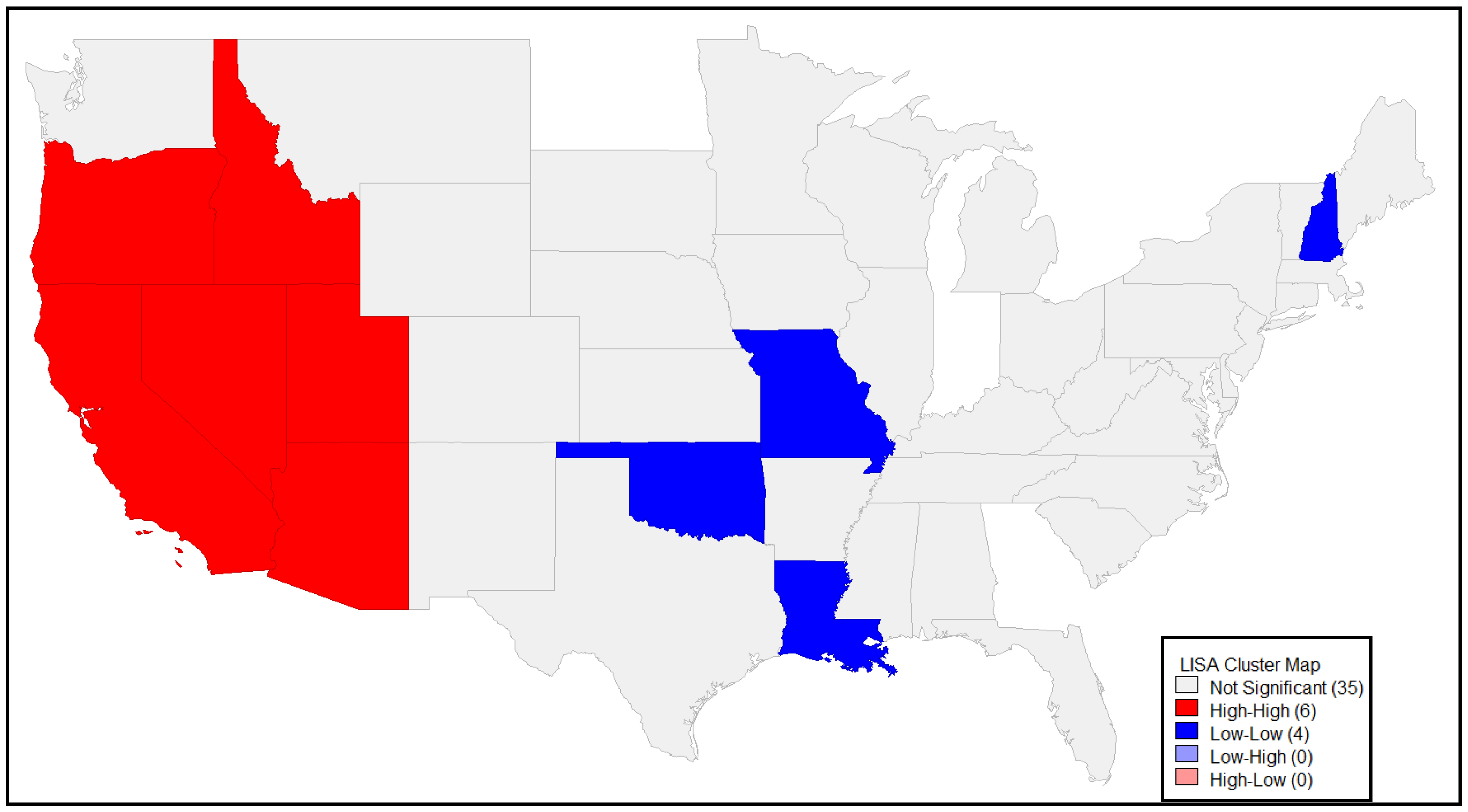
The LISA results in
Figure 2 for the unemployment rate growth clearly shows spatial clusters among the 45 states included in this study. Six western states form the core states in High-High (H-H) spatial clusters at 5% significant level (HH is shaded in red). These states are Oregon, California, Nevada, Arizona, Utah, and Idaho. These states show higher growth in unemployment rate change than the national average and are also surrounded by neighboring states with higher growth in unemployment rate changes than the national average based on the Rook contiguity weight matrix. Four states form the core states for Low-Low (L-L) spatial clusters at 5% significant level (LL, are shaded in blue). These states are Oklahoma, Missouri, Louisiana and New Hampshire, with lower unemployment rate growth than the overall national average, surrounded by neighboring states with lower unemployment rate growth than the overall average. None of the 45 states is classified as a statistically significant spatial outlier at 5% significance level.
Figure 2 shows a LISA map for the growth in unemployment rate variable.
6.2. Growth in TANF Caseload
We tested the global spatial distribution of the TANF caseload change during each state’s recession with Moran’s I statistics. The estimated Moran’s I statistics value of 0.1480 suggests a positive spatial autocorrelation, but it is not significant at 5% level with a pseudo p-value of 0.059420. As a result, we cannot reject the null hypothesis of random spatial distribution of TANF change at 5% significant level. Consequently, no global spatial association is detected at 5% significance level.
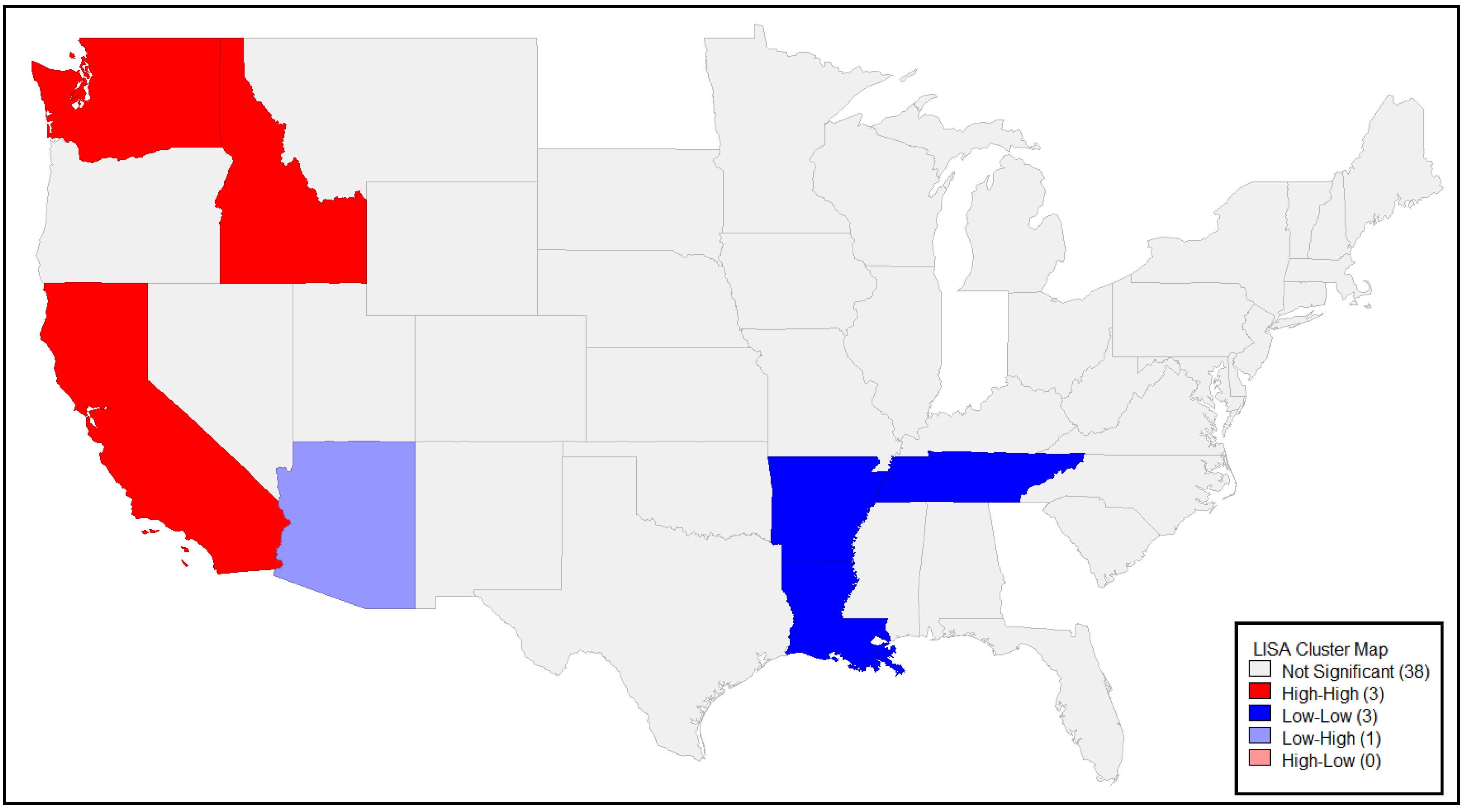
Figure 3, a LISA map, shows local spatial patterns for TANF changes among the 45 states included in this study. Six states form a spatial cluster at the 5% significant level. Three states in the West serve as core states for High-High clusters (Washington, Idaho, and California) and the other three in the South, are the core states with Low-Low clusters (Arkansas, Louisiana, and Tennessee). The High-High clusters in the west suggest high TANF caseload changes and that they are also surrounded by neighboring states with high TANF growth, based on the Rook contiguity neighbors weight matrix. The latter spatial clusters are found in three core states, which form Low-Low spatial clusters with low TANF growth of the three states surrounded by their neighbors with low TANF growth rate. Arizona is the only state classified as a spatial outlier at 5% significant level because its TANF change is much lower than the overall average among the 45 spatial units where its three neighboring states had higher TANF change compared to the overall average.
6.3. TANF Responsiveness Index
As described earlier, the responsiveness of TANF to the Great Recession is better captured when a state’s relative TANF growth rate during the recession is calculated as a share of the average selected states’ growth of TANF caseloads. This figure is then divided by a state’s relative percent growth in the number of unemployed as a share of the percent growth in the average number of unemployed in selected states as shown in Equation (1).
The Estimated Moran’s I statistics value of −0.011, indicates a potentially weak positive spatial autocorrelation for the spatial distribution of the TANF responsiveness to unemployment growth. However, based on the Rook contiguity neighbors weight matrix, pseudo p-value for global spatial autocorrelation is 0.299000, which results in accepting the null hypothesis of random spatial distribution of the responsiveness at 5% significant level. Consequently, in this case, we conclude that in this case there is no global spatial association.
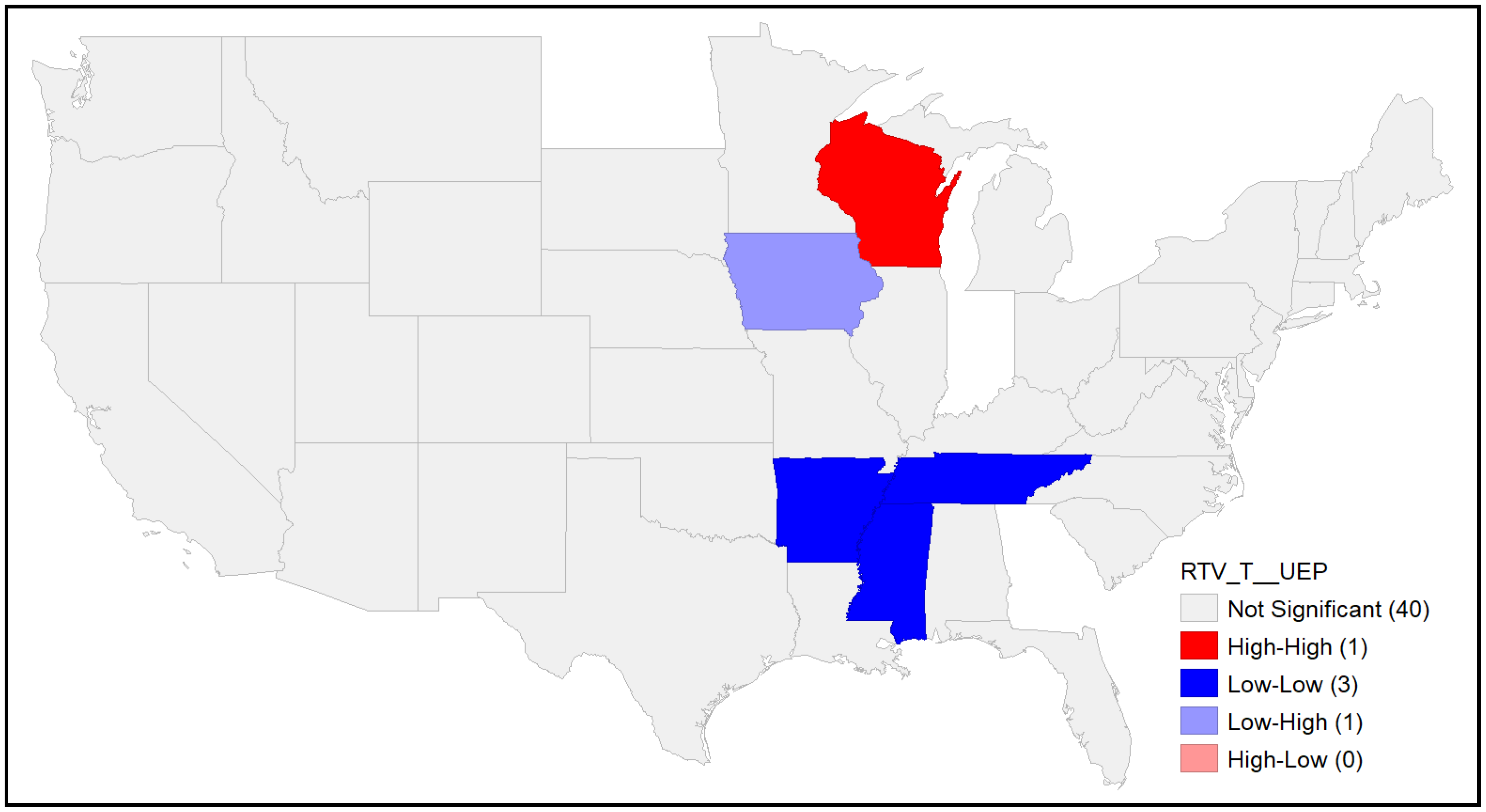
Figure 4 shows that we were able to detect the existence of a few spatial clusters based on LISA. Four states are found to be the core states of spatial clusters at 5% significant level. The state of Wisconsin, a core state, falls in High-High cluster (HH, shaded in red) because the state has high TANF responsiveness ratio and the average responsiveness of its neighboring states are higher than the average of the 45 sample states as well. States falling into a HH cluster can be defined as the states with a relatively higher TANF responsiveness rate than the overall average TANF responsiveness rate as well as being surrounded by neighboring states with higher than average TANF responsiveness rate.
The other three core states, Arkansas, Mississippi, and Tennessee, are states with Low-Low clusters in the South (LL, shaded in blue). The Low-Low cores states have a lower TANF responsiveness than overall average TANF responsiveness among the 45 sample states. Core states in this case are also surrounded by neighboring states with lower than average responsiveness. For example, Mississippi is a core state in the LL cluster with neighboring states of Alabama, Arkansas, Louisiana and Tennessee, all of which have lower than average TANF responsiveness. There is one spatial outlier state in the LISA map, which is Iowa (LH, shaded in purple) for the spatial distribution of TANF responsiveness. Iowa is a core state of Low-High, indicating it has relatively low TANF responsiveness, while the averaged TANF responsiveness among its neighboring states is higher than the overall average of 45 sample states.
6.4. States’ TANF Payment Levels (Maximum Aid)
Initially we analyzed spatial autocorrelations of several TANF policy variables, including TANF maximum aid, lifetime limits, sanctions, diversion payments or job search. Aside from TANF maximum aid, none of the other policy variables proved to have a statistically significant global spatial autocorrelation. Also, spatial patterns of these other policy variables at local levels were not quite strong. Therefore, we only present the results for TANF maximum aid (payment levels) here, which proved to have a statistically significant global spatial autocorrelation. We chose to apply spatial analyses to TANF maximum aid in real terms for a family of three (in 2007 US dollars). This variable was captured at TANF’s peak for each state. Studies have repeatedly shown that TANF maximum aid varied substantially among states, even when controlling for cost of living. During the Great Recession, several states cut their TANF benefit levels in nominal terms or simply let benefits erode with inflation. In contrast, there were some other states that chose to improve access to their programs by increasing their benefit levels or at least kept them up with inflation. This variable was chosen rather than other policy variables because the evidence is strong that this variable is a strong predictor of TANF enrollment.
We tested the global spatial autocorrelation for ‘maximum aid level at TANF peak’, measured in 2007 US dollars. Our findings reveal that the estimated Moran’s I statistics value was 0.6084 and that it is statistically significant at 1% level with pseudo p-value of 0.000010 based on the Rook contiguity neighbors weight matrix. Consequently, we reject the null hypothesis of random spatial distribution of the maximum aid at TANF peak at 1% significant level. We are confident that there is a positive global spatial association.
Of all variables tested here for global or local associations, we found strong spatial association for maximum aid. The findings suggest that there is a strong presence of LL spatial cluster in southern states and HH cluster in northeastern states (see LISA Map,
Figure 5). Nine southern states are found to be core states forming LL spatial clusters: Texas, Missouri, Arkansas, Louisiana, Mississippi, Alabama, Tennessee, Kentucky, and North Carolina.
As shown earlier, of these states, five states (Arkansas, Louisiana, Mississippi, Alabama, and Tennessee) also served as core states of Low-Low clusters with TANF responsiveness variable facing increasing numbers of unemployed. In a similar vein, six states in New England are found to be core states with High-High spatial clusters at 5% significant level, including Maine, New Hampshire, Vermont, Massachusetts, Connecticut and New York. These states show relatively higher maximum aid levels and are also surrounded by high maximum aid of neighboring states based on the Rook contiguity neighbors weight matrix. No spatial outliers were found among the 45 states.
7. Discussion
Our study improves on some earlier studies that analyzed TANF caseload changes and TANF policies during the 2008 recession in several ways. First, consistent with some earlier research, we argue that, in order to understand the 2008 recession, it is essential to examine the rise in unemployment rate in each state rather than use the NBER’s national official recession period. Second, and very importantly, we developed a unique standardized TANF responsiveness index that more accurately allows us to compare the responsiveness of TANF program to labor market performance during the 2008 recession of the selected states. Third, applying spatial statistical tools, we tested for spatial regimes. These spatial analytical tools allowed us to determine the extent to which there have been regional and state-level variations regarding states’ TANF payment levels (maximum aid), unemployment rates, and TANF responsiveness to the 2008 recession.
The standardized responsiveness index reveals that most of the western states had ratios greater than one, which means that they were responsive to the recession. In contrast, the measure suggests that Arizona with ratio below one, was unresponsive to the recession. In other words, while Arizona’s unemployment rate increased substantially, its TANF caseload increased very modestly. The same thing can be said for several southern states such as Florida, Louisiana, Arkansas, Tennessee or Kentucky.
While we tested for spatial distribution patterns of a number of policy variables, TANF benefit levels was the only policy variable that proved to be statistically significant at a global level and confirmed the presence of spatial clusters. In southern states there is a strong presence of Low-Low spatial clusters of TANF benefit levels while there is a High-High cluster in northeastern states, which is consistent with earlier findings conducted in non-recessionary periods [
6]. Several neighboring states with low benefit levels in the South region have been known to have less of a financial commitment to poor families and children for several reasons including cost of living. In contrast, several neighboring states with high benefit levels in the northeast continue to have financial commitment to the poor during the recession as they have prior to the recession.
Our findings further show the presence of strong spatial clusters in the case of the unemployment rate at both global and local levels. For example, in the West region, six states were surrounded by neighbors that experienced high growths in unemployment rates (p < 0.05). Yet, the fact that there were no strong spatial clusters in the case of TANF responsiveness to labor market performance supports the notion that neighboring states’ programs do not necessarily respond in a similar way as their neighbors to needs of poor families with children.
8. Conclusions
The merits of applying spatial analyses to a social program like TANF that is designed and administered largely by states and localities are unveiled in the present paper. The spatial analyses in this study provided us with an understanding of some of the social inequities that occur when the TANF program and policies vary substantially state-to-state. One source of inequity was found when states witnessed similar sharp increases in unemployment rates yet dissimilar TANF responsiveness.
Almost all western states had a high responsiveness score (greater than one) in the midst of sharply rising unemployment but the same was not found in many southern states that also had sharp increases in unemployment. All else constant, this may mean that many poor families with children in need of cash assistance in the selected southern states were worse off during the recession than similarly situated families in the West region.
If the federal government wants states to become more responsive to the needs of poor families with children and minimize horizontal inequities, especially during economic downturns, it needs to measure responsiveness in the most accurate way possible. Using the index developed in this study is a good way to measure responsiveness. After using the responsiveness index, when the federal government witnesses such inequities, it needs to try to identify reasons for low responsiveness. Is it that the states with low responsiveness scores are deterring eligible families from applying for aid or remaining on aid? Is it that these states are facing revenue shortages which impede them from fully serving their eligible populations?
Clearly the federal government may try to aid with states’ revenue shortages. The federal government should find ways to financially assist states that are not responsive to their poor families during the recession. Another solution, but a more extreme one, would be for the federal government to reduce the strong roles that state and local government have in the design and administration of TANF. While this idea is contrary to the one accompanying welfare reform efforts which granted states and local authorities a great deal of flexibility in the design and implementation of their TANF, the inequities that existed prior to welfare reform have only been exacerbated.
The extent to which horizontal inequities prevail in the TANF program and its policies are further evidenced when spatial analysis is applied. While almost all states have decreased their benefits in real terms, benefits are relatively higher in many northern states. In the case of TANF benefit levels, spatial analyses show that neighboring states do pay attention to their neighbors’ benefit levels. This finding suggests that many states may be competitive and cautious about setting benefit levels. Once again, this calls for increasing federal government responsibility in minimizing horizontal inequities by taking more control of TANF program rather than less control, as has been the case since 1996. Researchers in the past suggested that the federal government should be in control of redistributive programs rather than state or local governments [
26].
The present study also leads us to think about future research directions. First, because this study was conducted during the 2008 recession, future research should be devoted to repeating this study during a nonrecessionary period. A spatial temporal approach can be used to examine changes in selected variables over time. Second, since in some states, for example, California, there is a great deal of variation on a county level in the administration of the TANF program, spatial analysis could be applied using the counties as the units of analysis. This will allow us to examine inequities within a state. Third, a similar spatial approach taken for the present study can be applied to other TANF outcomes, including states’ TANF expenditures per capita.
Taken together, the present study’s findings have confirmed that idea that spatial analyses can be useful for policy research. In the era of evidence-based policy making, the role of spatial analyses is bound to expand.


