Performance Degradation Model for Concrete Deck of Bridge Using Pseudo-LSTM

Abstract

The purpose of a bridge maintenance strategy is to make effective decisions by evaluating current performance and predicting future conditions of the bridge. The social cost because of the rapid increase in the number of decrepit bridges. The current bridge maintenance system relies on traditional man-power-based methods, which determine the bridge performance by employing a material deterioration model, and thus shows uncertainty in predicting the bridge performance. In this study, a new type of performance degradation model is developed using the actual concrete deck condition index (or grade) data of the general bridge inspection history database (1995–2017) on the national road bridge of the bridge management system in Korea. The developed model uses the long short-term memory algorithm, which is a type of recurrent neural network, as well as layer normalization and label smoothing to improve the applicability of basic data. This model can express the discrete historical degradation indices in continuous form according to the service life. In addition, it enables the prediction of bridge performance by using only basic information about new and existing bridges.

1. Introduction

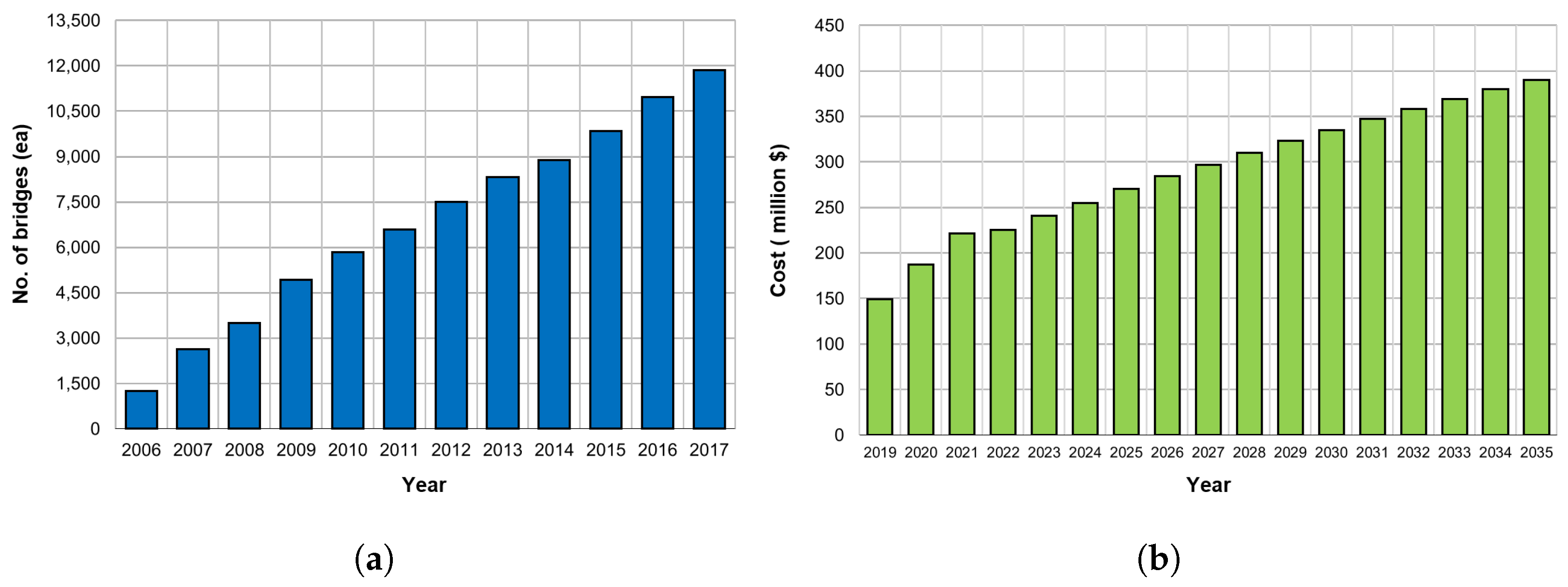
With economic growth and industrial development, the number of bridges has increased rapidly globally. In developed countries, such as the United States and Japan, deterioration of structures gained concern since in the 1900s and is expected to rapidly begin in Korean bridges from 2020. The increase in the number of deteriorated bridges causes difficulties in maintenance, thus increasing the cost of maintenance and reinforcement. According to the “Road Bridge and Tunnel Statistics” of the Ministries of Land, Infrastructure and Transport in Korea, the number of national road bridges continued to increase from 2006 to 2017 [1], and the total cost of maintenance of structures will gradually increase, as shown in Figure 1 [2]. Additionally, the lack of skilled personnel, discrete condition index criteria, and visual inspection of bridges result in high uncertainty and error. Bridges that are not properly managed have poor serviceability, leading to unusable bridges.For these reasons, bridges that have not been properly managed have caused several major accidents, resulting in numerous mass mortality events and considerable property damage. In other words, the end of service life or collapse of a bridge not only causes loss of life but also paralysis of the city, which can cause huge economic losses. To prevent such damage, bridges and facility maintenance are being actively studied. Recently, various studies have been conducted to improve the previous man-power-based facility inspection system through the construction of a maintenance system using unmanned test equipment, robots, and sensors [3,4,5]. In addition, the development of image processing and deep learning, combined with unmanned inspection techniques, has led to the quantification of deteriorated states, such as cracks, leaks, and corrosion [6,7,8,9].

The deterioration of places that are difficult for people to approach extracts quantitative figures with considerable levels of resolution with only photographs or technical images. Therefore, if effective algorithms; hardware, such as Internet of Things (IoT) devices; and unmanned inspection equipment are developed, an unmanned inspection system can soon be constructed [3]. To effectively manage a bridge, it is necessary to judge its current performance based on the inspected data and to predict the future performance based on its current state. However, it is still difficult to evaluate the performance of bridges using quantified deterioration data. Until now, the evaluation of the state of bridges depended on the performance model of the material used, as well as expert judgment [10,11,12,13].

In addition, durability of concrete materials as well as direction and limitations of service life prediction have been suggested through many studies [14]. Since the 1970s various bridge performance prediction models have been developed and grade prediction has been conducted using the classification and regression tree(CART) method, with the National Bridge Inventory (NBI) condition ratings and the Commonly Recognized (CoRe) data in the United States [15]. A study to predict the NBI condition rating was also conducted by Hasan [16], using the regression method and Monte Carlo simulation method to build four structures of PSC bridges in California (slab, stringer/multi-beam or girder, T-beam, and box beam or girder). Kong [17] researched the reliability-based prediction of the lifecycle reliability performance, cost, and optimal maintenance interventions of deteriorating structural systems. Huang [18] extracted 11 influence factors of concrete decks, and predicted related deterioration using and artificial neural network(ANN) model based on Wisonsin‘s BMS data. Lee [19] developed a deterioration model of the PSCI girder bridge by using a stochastic Bayesian update model. Bridge performance models using various algorithms are being developed, using considerable data, and mathematical and statistical techniques.

With the recently growing interest in the big data field, a bridge performance model using a neural network is being developed. Fathalla [20] showed the failure model of RC bridge decks through a finite element method model and the remaining fatigue life using an ANN. Tokdemir [21] developed a performance prediction model that applied an ANN and a genetic algorithm based on the highway bridge condition rating of the California Department of Transportation. Similar cases were conducted in Missouri and Alabama states, using data from the Federal Highway Administration (FHWA) of the US Department of Transportation and the NBI database as the basic data. In addition, a bridge deterioration model for each research was developed using a simple neural network [22]. However, in studies conducted using ANN-applied models, a large standard deviation occurred in the expected results for each grade; moreover, a specific result value could not be predicted for decision-making.

In the Recurrent Neural Network (RNN) model used in this study, parameters affecting the bridge structure are considered the influence factors. After Scherer [23] used the Markov chain model to derive the influence factors of an entire bridge, Su [24] derived the influence factors by using the logistic regression model. Recently, Lim [25] derived the influence factors using big data-based Xgboost. When confined to a concrete deck, the influence factors were derived using a case-based reasoning method [26], and Melhem [27] using the decision tree model was conducted. In addition, Huang [28] used a neural network model to derive the influence factors of concrete decks. Nabizadeh [29] developed a hypertabastic survival model using key influence factors with actual NBI records from Wisconsin. Previous research [25] cases have indicated that bridges are complex structures comprising environmental, identification, structural, and inspection factors. The relevant information utilized in this research [25] was also obtained from the basic bridge design information, and statistical data were used as the weather and vehicle load data. The basic data used in this study were the concrete deck inspection results obatained from the precise diagnosis and precise safety diagnosis of the national road bridges in Korea(1995–2017). The long short-term memory(LSTM) algorithm, which is a representative RNN model, was utilized for model generation [30]. To improve the model performance, several methods were used to take into account the measurement errors that occurred during the actual inspection. Finally, to verify the applicability of the developed performance degradation model, the actual bridge information was entered into the model to check the shape of the model.

2. Datasets

2.1. Introduction of Datasets

This section describes the data used in this study and their preprocessing conducted for model development. The database of the national road bridge precise diagnosis and precise safety diagnosis in Korea was used to develop a performance degradation model for a concrete deck. In general, bridge inspection is divided into regular inspection, precise diagnosis, precise safety diagnosis, and emergency inspection. Among these, precise safety diagnosis and precise diagnosis data relatively more reliable, and hence used in this study. Precise diagnosis indicates that a person with experience and skill examines the inherent risk factors by examining them with the naked eye or using inspection equipment. In case of precise safety diagnosis, it is recommended to investigate, measure, and evaluate the structural safety and causes of defects, to suggest repair and reinforcement methods The purpose of precise diagnosis and precise safety diagnosis is to find physical and functional defects and inherent risk factors of facilities through field surveys and various tests, and to provide prompt and appropriate repair and reinforcement methods and measures for such facilities. The ultimate aim is to ensure safety.

In Korea, in the 1990s, the collapse of the Seong-su Bridge and Sam-poong Department Store established the importance of safety management. Accordingly, in 1995, the government enacted the Special law on the Safety and Maintenance of Facilities to implement the safety management of facilities. In particular, to standardize the safety inspection and precision safety diagnosis of facilities, guidelines were provided for the methods and procedures for inspection and diagnosis of 12 major facilities in the country, such as bridges and dams [31]. Accordingly, the state history database has been developed by collecting the data of national road bridges since 1995, and the database accumulated up to 2017 contains the condition indices data of 350,384 bridge representative members. This dataset is the condition indices data for bridges built after 1995 and compress 10 representative members and 69 detailed representative members.

Table 1. Configuration of the bridge members state history data.

CALS *	B07	B08	B11	B16	B17	…
Elements Name	Deck	Girders	Secondary Members	Piers	Abutment	…
Amount of Data (ea)	75,524	56,118	50,521	55,468	19,676	…

CALS *: Continuous Acquisition and Life-cycle Support.

lists the configuration of the data for each member.

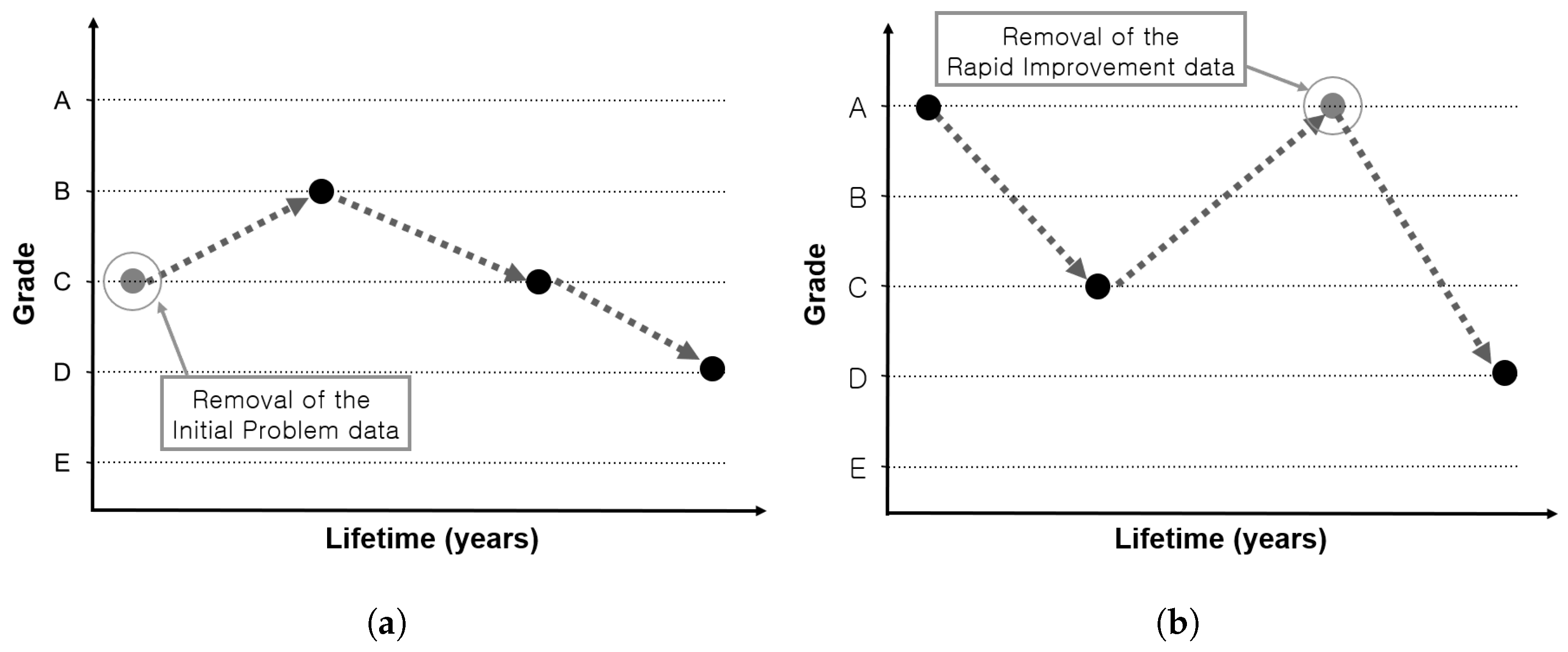
Although the database gradually accumulates considerable data, its reliability is low because the division of maintenance and reinforcement data before 2008 is not clear. Similarly, since 2008, many cases of maintenance and reinforcement have not been specifically provided. Therefore, to improve the reliability of data in this study, if there is historical information with an improved condition index because of maintenance measures (reinforcement, replacement) in each span, the data collected after the action are deleted. In addition, as the distinction between repair and reinforcement is often unclear, the data collected after the condition index has been upgraded by two or more grades are considered as data collected after the measurement; hence, they are deleted. After this process, the initial faulty data with condition index immediately after the construction below the C grade are filtered out as abnormal data. C grade refers to a condition in which minor defects in the main member or a wide range of defects occur in the auxiliary member, but safety is not impaired. It covers cases where maintenance is required to prevent degradation of durability and functionality of the main member, or when simple reinforcement is required on the auxiliary member. Figure 2 shows examples of the data with initial faulty and abnormally rapid grade improvement.

So far, the data preprocessing has aimed to improve the reliability of data and use only the no-action data, except for repair and reinforcement measures. The use of data in case of non-action is due to the possibility of grade increase in case of repair or reinforcement.

2.2. Detailed Information on Concrete Deck Inspection Data

This study finally aims to develop a bridge performance degradation model. However, bridges are a combination of various members and can be designed in various forms, lengths, and widths, depending on the surrounding natural conditions. Thus, to develop a generalized bridge performance model, member-specific model development should precede.

Therefore, the database is classified based on members;

Table 2. Configuration of the deck plate data.

SBCode *	001	003	006	008	009	099
Elements Name	Concrete Deck	PSC Deck	Concrete Slab	Hollow Concrete Slab	Hollow PSC Slab	ETC
Amount of Data (ea)	58,554	2620	12,484	1148	168	550

SBCode *: Detailed element code.

lists the configuration of the deck plate data. According to Table 2, concrete deck data has the largest number. In general, the most commonly used concrete deck data has the largest amount of data, which indicates it can be utilized most effectively in big data analysis. In other words, the data to be used for the model development is the condition index of the concrete deck and is applied to the model after the above mentioned preprocessing. 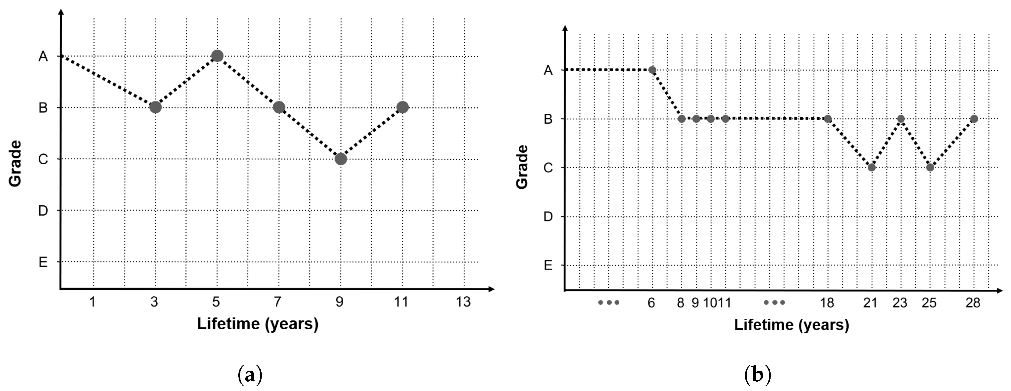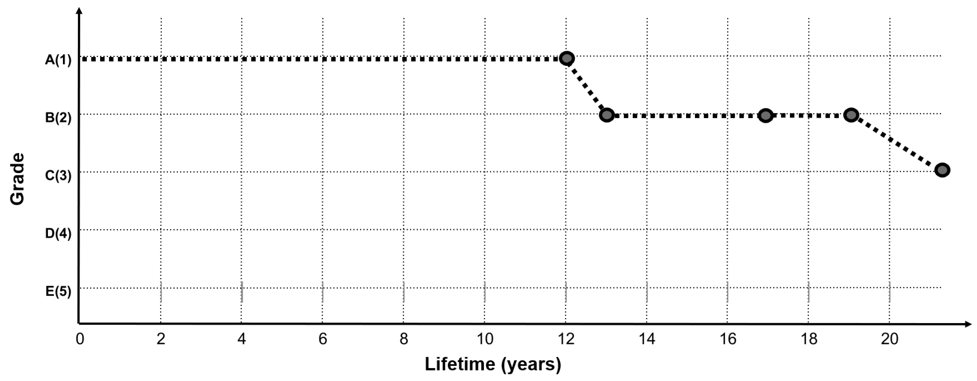Figure 3 shows an example graph of the concrete deck condition index history of two bridges (Gal-Cheon Bridge and Chun-Sung Bridge), among the final preprocessed data.

In the graph of the two bridges shown in Figure 3, the condition index history data show irregular shapes, which are not continuous, depending on the service life. The reasons for obtaining this shape are as follows. First, bridge inspections are not carried out continuously by the same inspectors every year or at regular intervals. Second, there is judgment error from the inspectors, due to the discrete condition index criterion. Third, the measurement error of the visual inspection results from requiring a very small unit of measurement.

Table 3. Concrete decks safety performance evaluation standard in Korea.

	Crack		Deterioration/Damage
	1-Way	2-Way
a	Crack width: Under 0.1 mm	Map Cracking width: Under 0.1 mm	-
b	Crack width: 0.1–0.3 mm Crack ratio *: Under 2%	Map Cracking width: 0.1–0.3 mm	Surface damage area: Under 2%
c	Crack width: 0.3–0.5 mm Crack ratio: 2–10%	Map cracking width: Over 0.3 mm	Surface damage area: 2–10% Rebar corrosion area: Under 2%
d	Crack width: 0.5–1.0 mm Crack ratio: 10–20%	Concrete spalling due to crack propagation	Surface damage area: Over 10% Rebar corrosion area: Over 2%
e	Crack width: Over 1.0 mm Crack ratio: Over 20%	Possibility of punching failure due to spalling	Decreased safety of decks due to corrosion of rebar

* Crack ratio = Area of crack/Inspection Area * 100.

lists the concrete deck’s safety performance evaluation standards followed in Korea, in order to check the error caused by the discrete shape of the condition index standard. Because the grade is a discrete form that is suddenly divided at one point, errors will occur while selecting a grade. Additionally, such inspections are not continuously performed for a certain period by the same inspector. As the actual inspections are performed by independent inspectors, subjective errors occur in this part as well.

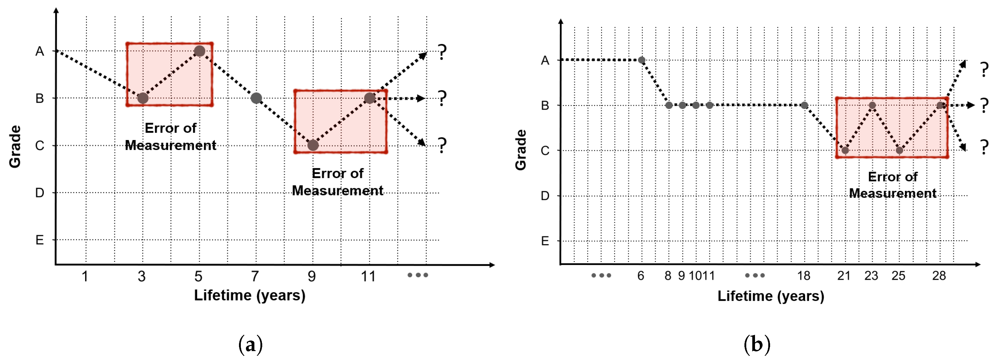
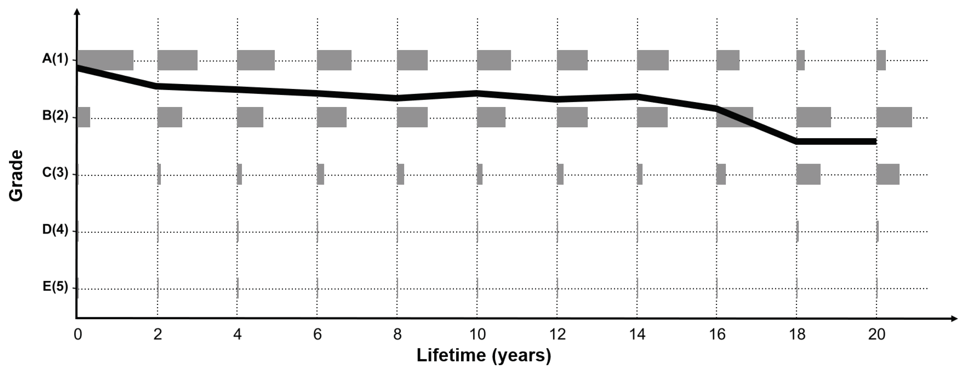
In addition, assuming that the state grades determined by cracks in the concrete deck are to be decided, the measurement unit for judging the state grade is too small, given the inspection condition by the current manpower. From the perspective of inspectors who have to check a wide range of decks, this can cause considerable judgment error. In areas that are difficult to access or dark areas where visibility is poor, it would be very difficult to determine the crack width in millimeters by the naked eye and subsequently decide the grade. These various inspection criterion problems and errors caused by the inspector’s judgment result in a jagged measurement error, as shown in the shaded part of Figure 4.

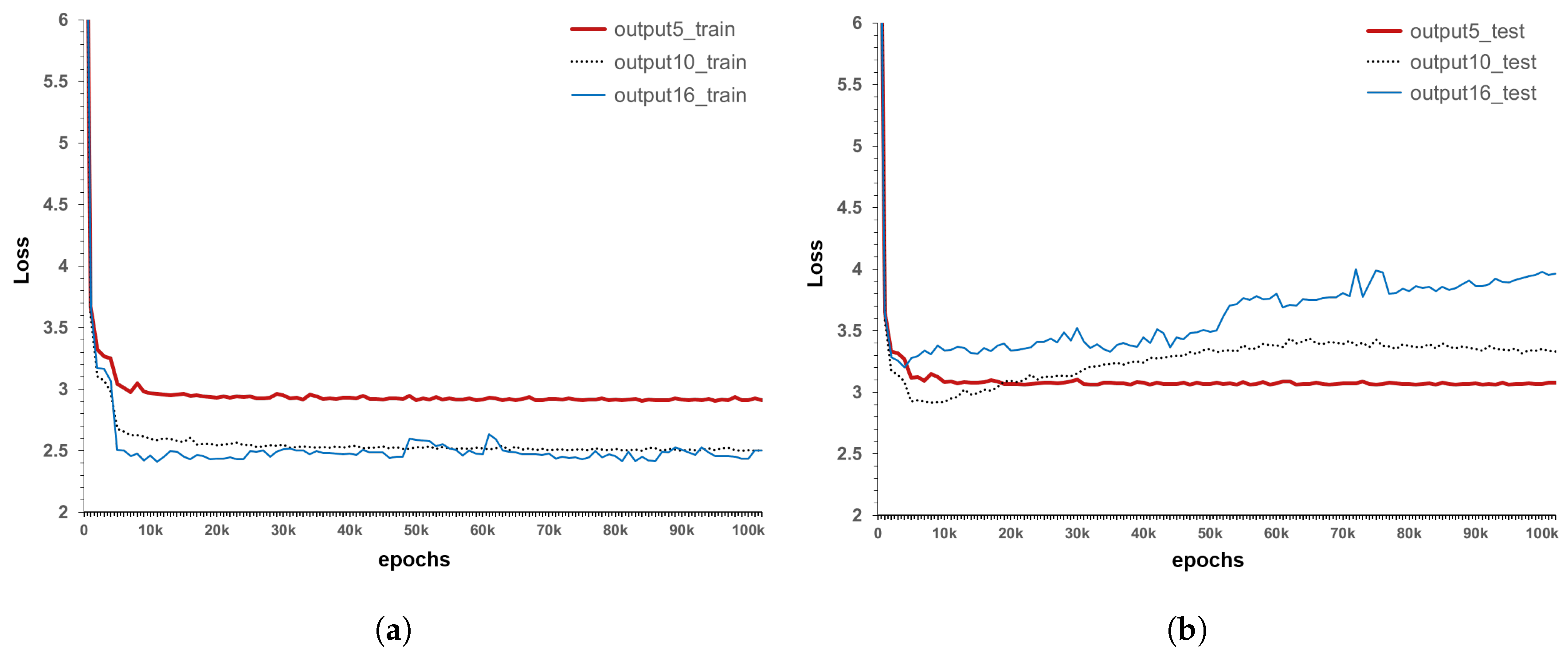
Many bridges do not show a constant grade change, and generally show a graph shape with a little measurement error, as indicated in Figure 4. Therefore, if the accumulated inspection data are used as such, the model accuracy will be decreased owing to measurement error. To address this issue, an alternative method is to consider the parts where the condition index change is abnormal as the measurement error. As the LSTM model to be developed requires sequential data, the data preprocessed according to the service life (inspection date–construction date) are classified into 11 sequences, with each sequence comprising two years of service life. The data after 20 years of service life are equally input to the last sequence. The reason why the final sequence is spread over 20 years, in the case of a bridge structure, is that it is difficult to secure long-term no-action data after 20 years of service life because maintenance and reinforcement measures are performed according to a certain level of inspection results.

2.3. Influence Factors

The factors influencing the bridge performance can be divided into design factors and environmental factors. First, the design factors refer to detailed specifications of the bridges that are presented in the design, which include the span length, total width of the bridge, thickness of the deck, and strength of the deck. The characteristics of the design factors have different unique values for each bridge, which do not change according to the service life. Second, environmental factors are considered as factors that affect the bridge condition. In the study of international bridge performance degradation models, the selection of factors was based on the type of influence factors considered [32]. Among the factors presented in the various studies, the main environmental influencing factors used in this study include the average daily truck traffic (ADTT), average chloride, and average humidity of the bridge. ADTT is obtained by collecting the annual average traffic data of each bridge through the statistical yearbook of the Korean Ministry of Land, Infrastructure and Transport [33]. In addition, the amount of surface chloride is calculated based on the average amount of deicer used in each region, while the average humidity value used in the study is obtained from the meteorological agency humidity statistics [34].

A total of 17 input parameters, comprising 14 design factors (height, continuity, type of girder, length of span, width, thickness of deck, strength of deck etc.) and 3 environmental factors (average daily truck traffic, average chloride, and average humidity), are used for the model development. Looking at some design factors, type of girder indicates girder such as PSCI, Steel box, Reinforced Concrete, etc and there are basic factors such as span and height. Information related to strength, thickness, and rebar indicating the properties of the deck are listed in the design factors, and continuity is a factor for dividing continuous and simple beam bridges. All influence factors are described in

Table 4. Influence factors.

Factors	Parameters
Environmental Factors	1. ADTT	2. Average Humidity	3. Chloride
Design Factors	4. Type of Girder	5. Number of Span	6. Length of Span
	7. Width	8. * Support Type	9. Strength of Deck
	10. Diameter of Rebar	11. Type of Overlay	12. Design Load
	13. Strength of Rebar	14. Thickness of Overlay	15. Height
	16. Thickness of Deck	17. Continuity

* Support type: Piers and Abutments.

.

Each value is normalized to minimize the effect of only a few factors affecting the model because of the absolute value difference. As actual bridges are a complex combination of various factors, only some specific factors can be considered to not affect the bridges. Therefore, various parameters related to the concrete deck are utilized as the input parameters.

3. Methods

3.1. Overall Architecture

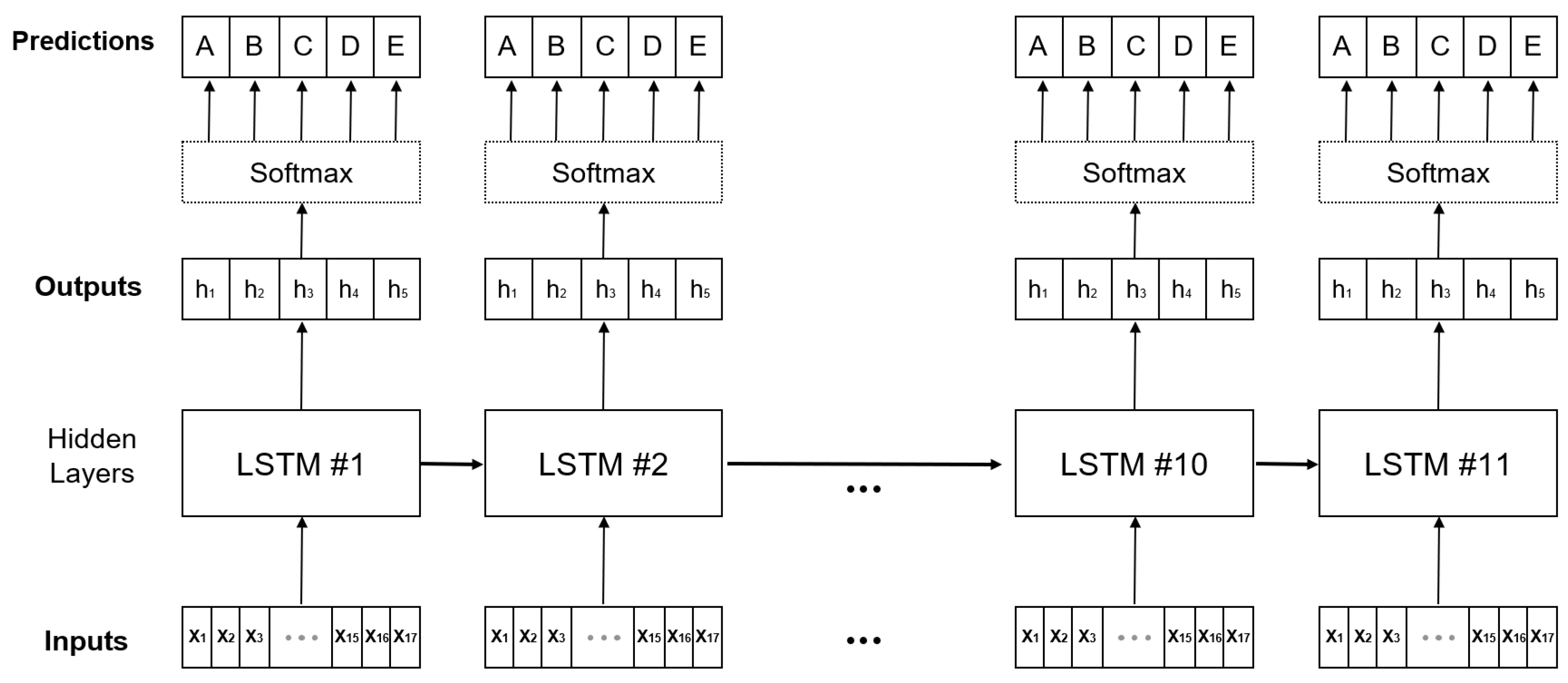
This section describes the algorithm and the overall architecture used to develop the model. To develop a model that shows a change in the condition index over time, the deep learning algorithm LSTM, which is known as the shape of the RNN, is used [30]. The basic idea of the algorithm is to process sequential data. In the case of LSTM, it is effective for model development because past information affects the future. The existing RNN algorithm is dependent on the input and output data over time; however, in this study, the regionally and environmentally independent concrete deck inspection data of several bridges are used simultaneously. Therefore, only the algorithm structure is used in the pseudo-form; the architecture of the developed model is shown in Figure 5.

The module of the model architecture (hidden layer) is the same as that of the existing LSTM structure, with only the label shape smoothened. Specifically, the model has 11 sequences of 2 years of service life, and for ease of convergence, it uses only one stack. As mentioned above, the cross-entropy as a loss function is used to measure the difference between the predictions through the Softmax function and the smoothened ground truth distribution. A parameter update technique called the Adam Optimizer iss utilized because it can adjust the direction and step size appropriately [35]. In addition, the Vanishing/Exploding Gradient problem, which can occur as the model transforms deeper into the RNN form, is resolved using the following three methods. The first is employing an RNN structure, which is called LSTM; second is layer normalization; and last is a type of noise robustness, which is called label smoothing. The deep RNN algorithm has a covariate shift problem, in which the output of each layer changes during training. Layer normalization is used together with the RNN algorithm to solve this problem and shorten the training time [36]. Finally, this model aims to predict the probability of occurrence of the five condition indices identified during the bridge inspection.

3.2. LSTM

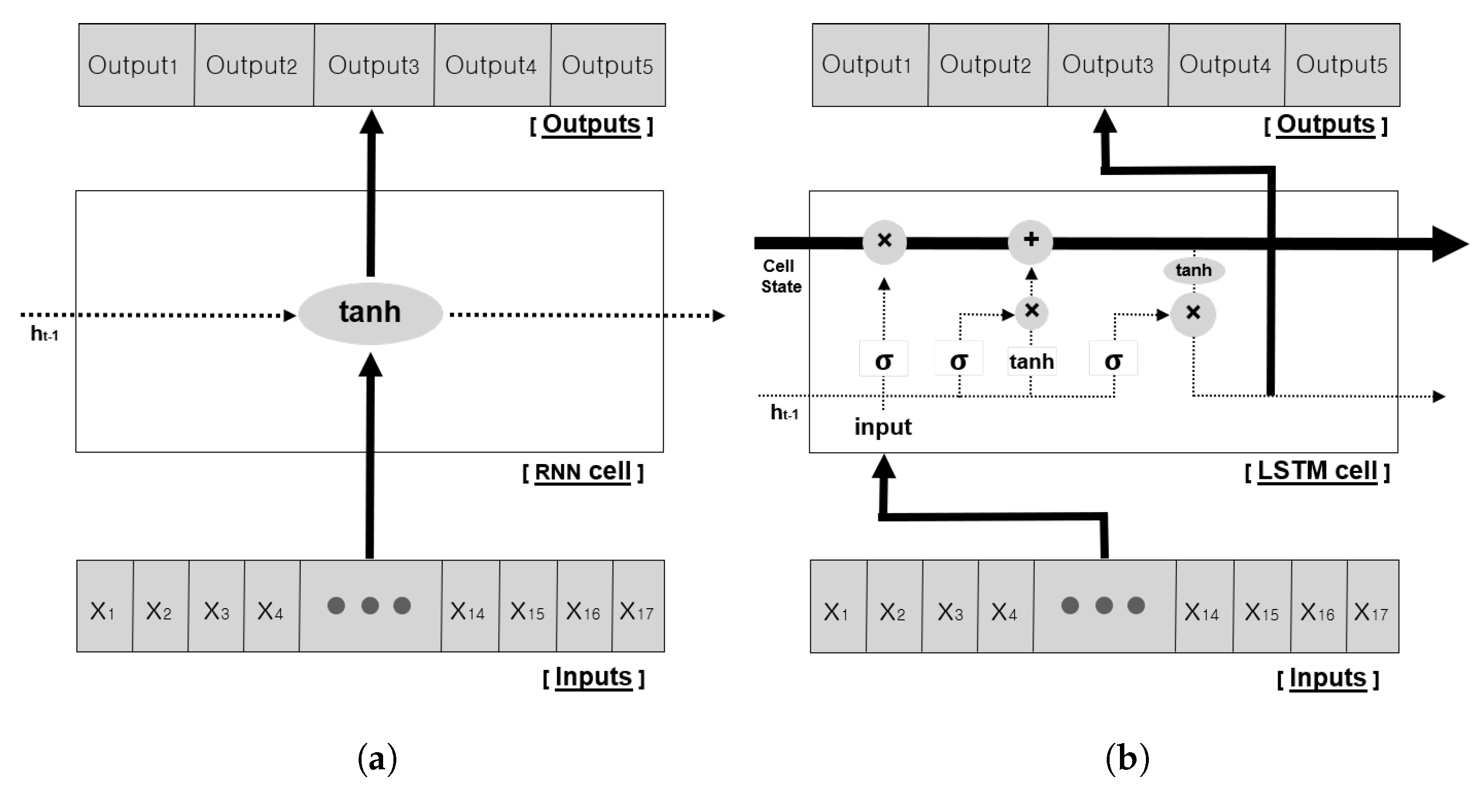
The RNN is a type of ANN where connections between hidden nodes form a recurrent structure. The initial RNN structure, which is called the vanilla RNN, comprises repeated chains of neural networks, where each module has a single hyperbolic tangent activation function layer structure.

Equation (1) and Figure 6a show that the hidden state $h_t$ which is updated inside the RNN, is affected by the existing state $h_{t-1}$ and the input $x_t$ [37]. The RNN structure can effectively process the sequence data, because the past information can affect the future, as follows:

$$h_t=f_w(h_{t-1},x_t)$$

(1)

$$h_t=tanh(W_{hh}·h_{t-1}+W_{xh}·x_t)$$

(2)

However, owing to this algorithm structure, as the distance between the past and future increases, the gradients gradually decrease or increase during backpropagation, and the training ability is significantly degraded. This phenomenon is called the vanishing/exploding Gradient Problem, and which occurs not only in the vanilla RNN structure, but also in the deep convolutional Neural Network structure.

To solve this long-term dependency problem, the LSTM algorithm is proposed [30]. LSTM has the same chain shape as that of the RNN; however, the repeated module has another a different structure with several gates added. In the existing RNN structure shown in Figure 6a, the hidden state $h_t$ of the current state is updated by the previous state $h_{t-1}$ and the input. However, instead of using a single neural network, the hidden state in LSTM has special gates inside the module, which interact with each another, as shown in Figure 6b. In addition, the cell state, which is the core idea of LSTM, helps to solve long-term dependency problems by sequentially connecting continuous hidden states. The gates in the module are divided into the Forget gate, Input gate, and Output gate (Equation (7)). First, the forget gate $f_t$ determines how much past information needs to be forgotten. It receives $h_{t-1}$ of the hidden state and input $x_t$ to determine the output value between 0 and 1, by taking the sigmoid activation function (Equation (3)):

$$f_t=\sigma (W_f[x_t,h_{t-1}]+b_f)$$

(3)

Second, the input gate determines how much input information to remember. Similar to the forget gate, it takes a sigmoid activation function with $h_{t-1}$ and input $x_t$, and additionally performs a hadamard product matrix operation with the hyperbolic tangent to the same input value (Equation (4)).

$$i_t=\sigma (W_i[x_t,h_{t-1}]+b_i)$$

(4)

$$g_t=tanh(W_g[x_t,h_{t-1}]+b_g)$$

(5)

Third, the output gate is an internal gate that determines how much to output to the current state. In other words, it decides how much information to output in the current state from the cell state. In this process, similar to other gates, it takes $h_{t-1}$ and input $x_t$ to derive the $o_t$ value through the sigmoid activation layer (Equation (6)). Then, the active function $tanh$ is applied to the cell state information updated in advance, and the result of multiplication with the $o_t$ value is the current state output ($h_t$) (Equation (8)). The $h_t$ value represents the current output, and acts as $h_{t-1}$ in the next sequence.

$$o_t=\sigma (W_o[x_t,h_{t-1}]+b_o)$$

(6)

$$c_t=f_t\odot c_{t-1}+i_t\odot g_t$$

(7)

$$h_t=o_t\ast f\left(c_t\right)$$

(8)

As mentioned above, the core of LSTM is called the Cell State, which updates the past and current information through the forget and input gates. As shown in Figure 6b, the cell state is a structure that penetrates the entire chain. This structure minimizes the loss of information, and allows it to transmit data to all sequences. This structural feature of LSTM makes it possible to solve the long-term dependency problem and has been widely used to process sequential information (e.g., natural language, stock prediction, and weather forecasting) [38,39,40].

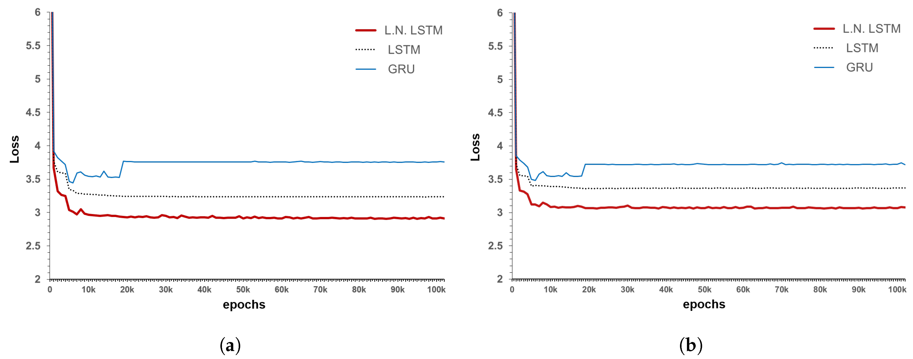
3.3. Layer Normalization

Deep-learning algorithms are generally not easy to train, because of the vanishing/exploding gradient that occurs in most models as the layers deepen. Then, in the case of a deep network, the distribution of the middle layer is shifted by the covariate shift phenomenon, in which the output distribution of each layer is changed with each training. Because of this phenomenon, the parameters are updated in the wrong direction, and the training does not progress smoothly [41]. Various methods have been developed to solve this chronic problem, and have helped in performance improvement. 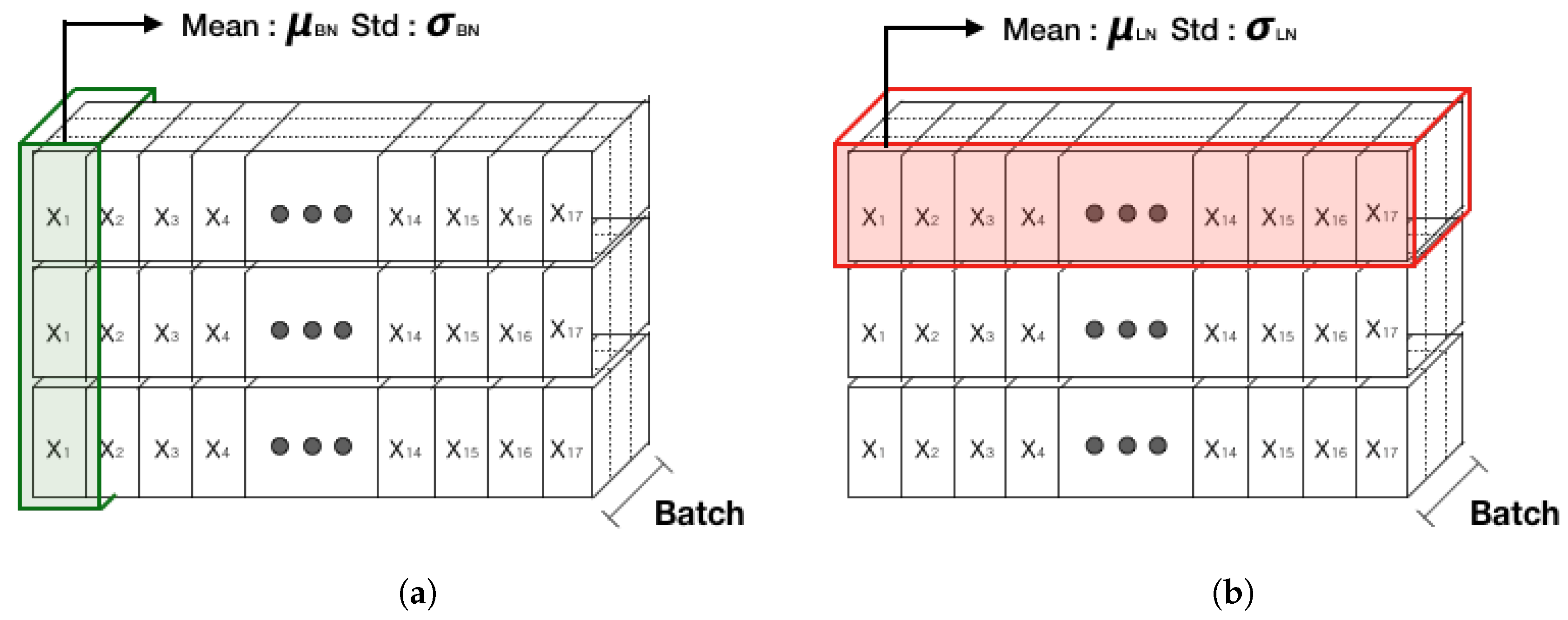Among these, the validated normalization technique used in most models is a method of normalizing the input and output, such as Batch Normalization, Weight Normalization, and Layer Normalization [36,41,42]. In fact, the above studies have been validated empirically and have many advantages in terms of training time and accuracy as well as solving Vanishing/Exploding Gradient problems. Batch normalization, which is widely used in the CNN model, is a method for normalizing the activation and output values of the hidden layer, such that the average is 0 and variance is 1. A technique for adding a little noise is to normalize the batch data at each layer of the neural network. However, as batch normalization requires normalization for each batch, the average and variance of the batch data might be different from that of overall data. It is difficult to configure a small correlation between the mini-batch sets to represent the whole data. In addition, the case of batch normalization does not empirically operate well in an RNN. Because of the difficulty in applying an RNN, a normalization technique that works well in the RNN algorithm, which is called layer normalization, has been developed. This method aims to improve the training efficiency of the deep RNNs by using a large learning rate and an additional simple layer. Figure 7 shows a comparison between batch normalization and layer normalization.

Layer normalization performs normalization among neurons in the same layer and is usable for RNNs because there is no dependency between the mini-batch samples. Through these analyses and tests, long-sequence RNNs and small mini-batches are found to have many advantages [36]. In this study, by additionally applying layer normalization in the LSTM structure, the changes in the training and test results can be presented.

3.4. Label-Smoothing

The data used in this study are the inspection data of the concrete deck for each span of bridges. The inspection data contain errors, such as the grade division error and the decision error. The grade division error refers to an error that occurs because the classification of the current bridge member is too discrete. Meanwhile, the decision error indicates an error caused by the subjective decision of the inspectors. Therefore, when the model is trained using the current inspection data as such, a model incurring several errors is developed. To address this issue, a type of noise robustness technique, called “label-smoothing” is used. This technique converts the previous binary inspection grades A, B, C, D, and E into the distribution form, and helps to make effective predictions without interfering with the correct classification [30,43]. The current accumulated bridge inspection data are independent from many general bridge inspection companies. This means that the same deterioration can be judged differently, depending on the company, inspection devices, and the inspector. As a practical example, the inspection data of the concrete decks do not show a constant form of degradation, as indicated in Figure 3, due to the various causes of the above mentioned errors. 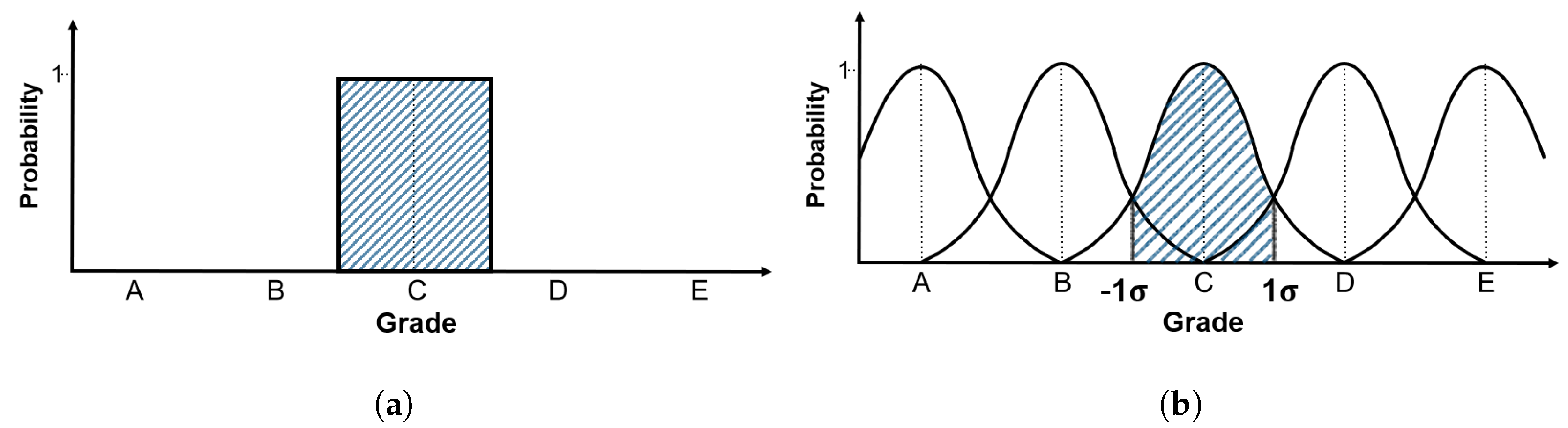In case of the Gal-Cheon Bridge shown in Figure 3, it is measured as grade B in the inspection conducted in the third year, which is raised to grade A in the fifth year. The same error is observed in the ninth and eleventh years and is similarly observed in the inspection data of various othor bridges. Therefore, when the performance degradation model using a data-based deep-learning algorithm is developed and trained, if the data showing such an error are used as such, training cannot be effectively performed. To consider the inspection errors caused by various reasons, label smoothing is applied to the condition indices of the inspection data. The label smoothing in this study is based on the central-limit theory, which states that if the number of samples is large enough, they are independent of each other and the average of the samples following the same distribution approximates a normal distribution. As a result, the existing status data are transformed into a standard normal distribution form, as shown in Figure 8.

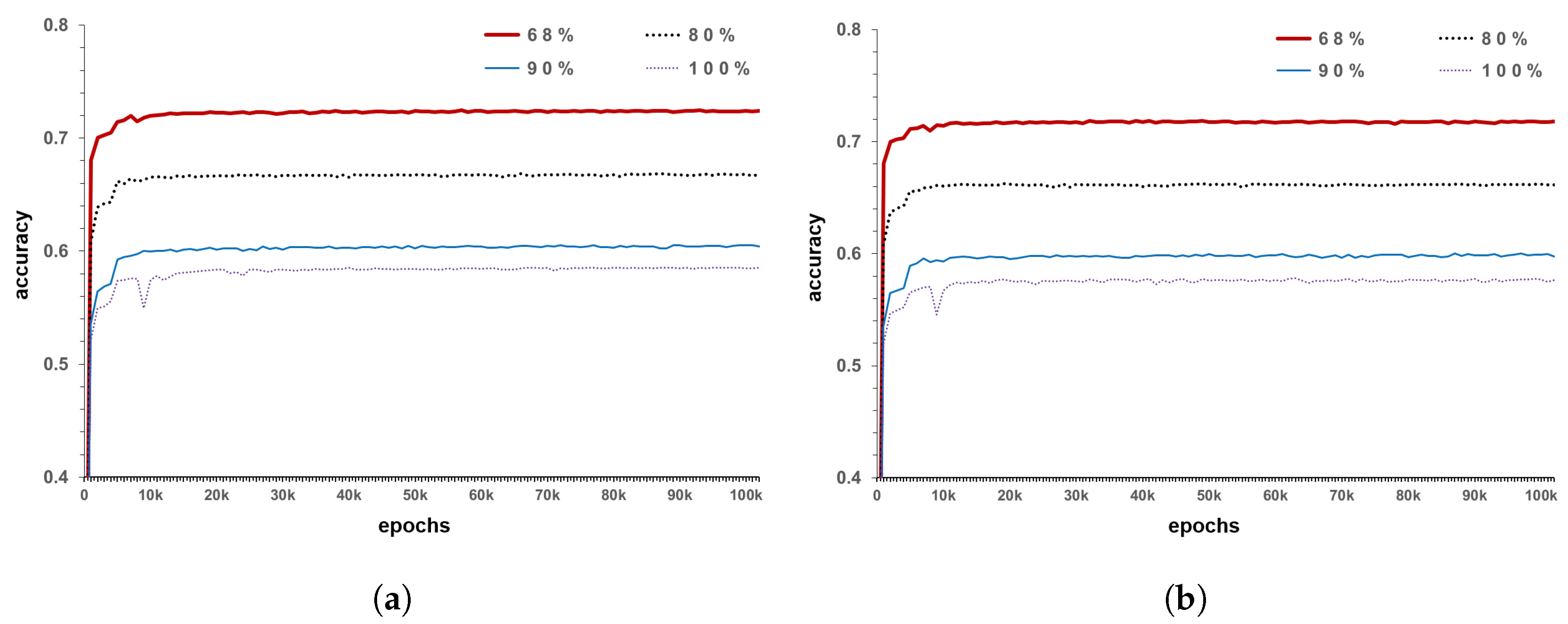
In the standard normal distribution curve, values of approximately 68% are present in one standard deviation range on both sides, while those of 95% are present within two standard deviation ranges. Standard deviation is a type of average error, which indicates how different the data are from the mean. Based on this concept, the measurement error is reflected. The method applies 100% confidence interval if the error is not reflected in the existing inspection data, 95% confidence interval when reflecting about 5%, and 68.3% confidence interval while considering error of approximately one-third. In other words, this expression indicates the amount of reflected measurement error of the current inspection data or amount of reflected accuracy of the existing data. Assuming that the average of the relevant inspection data is the measurement condition index, and that the one standard deviation is grade 1, it can be expressed as the standard normal distribution of 68.3% confidence interval. Likewise, if two standard deviation is assumed to be grade 1, it can be converted into a standard normal distribution with a 95% confidence interval. For example, as shown in Figure 8a, there are data measured in grade C for the existing inspection data. When applied to a model with 68% confidence interval, the probability of judging it as C is 68% and that of judging it as grade B or D is 16% (Figure 8b). This is to reflect the errors that occur during the inspection and various errors that may occur while determining the grade process, as mentioned above. In the current model, if the error is considered to be of the form ± 1$\sigma$ but the data accuracy is judged to be lower, the confidence interval may be further narrowed. The maximum error in the model is one-third. Lower values indicate that the reliability of the data themselves is too low to be statistically considerable. In the model development conducted in this study, a model with a confidence interval of 68.3%, which corresponds to a standard deviation of ±1$\sigma$, is generated as the minimum criterion, in order to take measurement errors into consideration.

3.5. Loss and Evaluation

The loss function for evaluating the degree of model training uses Cross Entropy (Equation (9)), which is often used as a multi-class classification loss function.

$$H(p,q)=-\sum _{i=1}^{n}p\left(x_i\right)log\left(q\left(x_i\right)\right)$$

(9)

The value of $p\left(x\right)$ in Equation (9) is the probability value of each label of the label-smoothing actual inspection data, and $q\left(x\right)$ is the prediction value passed through the Softmax layer. In the accuracy calculation process, as the value of the label has changed, the results are compared with the similarity of distribution, without using the conventional concept of binary accuracy. This is to show how well the distributed label is predicted. A maximum distribution similarity of 1 (100%) can be obtained by comparing the predicted value with the corresponding label, as shown in Equation (10).

$$DistributionSimilarity=-\frac{1}{sequence}\sum _{t=1}^{Sequence}\sum _{i=1}^{Classes}Min(h_{t_i},GroundTrut{h}_i)$$

(10)

The reason for applying the distribution similarity, instead of the existing accuracy, is that the existing data have too much error value, and if the data are used as such, training occurs in the wrong direction. The existing accuracy calculation cannot reflect the error because it is ignored, except for one value that is shown as the ground truth. In other words, if a previous accuracy equation is used, the training is performed such that the grade is increased owing to the data including the error; this becomes an issue. Conversely, measuring the distribution similarity regulates the ground truth value, assuming that little noise is contained in the existing data. Using the revised ground truth in training can partially reflect the measurement error values that can occur during the inspection. In addition, as the judgment error that may occur when a grade is determined can be reflected, a more realistic model can be developed.

4. Results

4.1. Training and Validation Results

The training process is conducted to develop the performance degradation model of the concrete deck on the national road bridge using several RNN models. For comparison, the LSTM algorithm applying layer normalization, general LSTM, and Gated Recurrent Unit (GRU) is used. The total data are split into two sets: 80% of the data are used for training and the rest are separated into validation and test sets. To train the optimal hyper-parameters, training is performed by the same epoch and the learning rate of Adam optimizer is fixed at 0.1. Figure 9 shows the loss results of training and testing for the LSTM algorithm obtained by applying layer normalization, general LSTM, and GRU:

As a result, the LSTM algorithm applying layer normalization shows the highest performance in training and testing of this model, followed by the general LSTM and GRU. In case of the GRU algorithm, the loss value after the early-stage iteration increases. Thus, layer normalization is effective in the RNN algorithm structure. Therefore, LSTM applying layer normalization (L.N LSTM) is basically used as a model for comparing the hyper-parameters. Second, Figure 10 shows the result according to the change in output size through the LN-LSTM module for each sequence of the algorithm. Generally, the larger the size of the output, the more the characteristics of the input parameters that can be reflected and the higher the accuracy. However, excessive overfitting can sometimes occur, depending on the output size. To examine these, the output size comprises (5, 10, and 16), and the results are obtained by training and testing.

Figure 10 shows that as the output size increases, the training loss decreases. Conversely, the loss value in the test shows a typical form of overfitting that increases with the output size. In case of a model with a few outputs, stable training and testing are performed.

These results show that although the bridge inspection data are composed of various influencing factors, it can be indirectly confirmed that not all factors directly affect the condition index.

Finally, Figure 11 shows the results according to whether label smoothing is applied. Training and testing are performed on the ±1 sigma model (68%), confidence interval model 80%, ±2 sigma model (95%), and the model that does not reflect the error. The ±1 sigma model is considered to reflect the measurement error of about one-third the inspection data. In this case, the similarity of the distributions is compared, because when the label smoothing is performed, the shape and reference points of the loss function are different for each item.

Figure 11 shows that the result of the distribution similarity is high for the 68% model, and if the ground-truth value is used without reflecting the error, the distribution similarity is the lowest. This means that the error of the inspection data is large, and it is appropriate to apply label smoothing to reflect the error in the actual data. To examine the validity of the distribution similarity, a model using the existing accuracy equation with the same hyper-parameters is created. Then, Figure 12 shows the result of the loss. In the case of the model with the existing accuracy equation, overfitting is observed during the test. Therefore, the existing accuracy model cannot be used as such. To solve this problem, the similarity of distribution is used.

As a result, the variance of the existing data is too large; therefore, even if the training progresses, the test data do not converge. When the model is created using the previous inspection data, it is difficult to use the existing accuracy as an evaluation tool without reflecting the error. This is because the error of the data itself is large, and a consistent test result cannot be achieved.

Therefore, the final model selected considering various factors is the LSTM structure using layer normalization; the output size is 5, and the label smoothing is applied. Figure 13 shows the results of the loss function and the distribution similarity in the training and testing of this model.

In other words, the developed model shows 71.9% similarity of distribution without the problem of overfitting, which considers a certain level of measurement error. In the next section, the developed model will be used to create a performance degradation model for actual bridges.

4.2. Tests for Actual Bridges

Once the training is completed, the input values of the actual bridge are inserted, and it is tested on the trained model. First, the 000001 Jin-Wui Bridge is determined as the target bridge. It was constructed in 1986 and is a five-span PSCI-type bridge.

Table 5. Input parameters of Jin-Wui Bridge.

Parameters	ADTT (ea/year)	Average Humidity (%)	Chloride (kg/cm${}^2$)	Design Load	Height (m)	Continuity
Data (ea)	46.952	68.41	5.45	DB-24	4.6	Continuity
Parameters	Type	Number of Span (ea)	Length of Span (m)	Width (m)	Support Type *	Thickness of Deck (mm)
Data (ea)	PSCI	5	25	19.5	1	200
Parameters	Strength of Deck (kgf/cm${}^2$)	Diameter of Rebar (mm)	Strength of Rebar (N/mm${}^2$)	Type of Overlay	Thickness of Overlay (cm)
Data (ea)	270	22	400	Asphalt	5

* Support type: Piers and Abutments.

shows the parameters of the bridge to be input to the developed model.

As a result of the actual inspection based on the year 2018, the bridge inspection is conducted at the service life of 12, 13, 17, 19, and 21 years. The change in the grade of the Jin-Wui Bridge can be observed in Figure 14; as in the previous example, there is no performance degradation of a certain shape.

To overcome this problem, a model has been developed, to which the parameters of each bridge can be input to the developed model to derive a constant grade-change model of a specific bridge. In the developed model, only the actual parameters of Jin-Wui Bridge are input to all sequences, and

Table 6. Estimated probability of each grade in Jin-Wui Bridge‘s concrete deck.

Lifetime (Years)	0–1	2–3	4–5	6–7	8–9	10–11	12–13	14–15	16–17	18–19	20
A	0.814	0.585	0.548	0.495	0.453	0.500	0.441	0.460	0.330	0.119	0.130
B	0.186	0.359	0.385	0.428	0.448	0.419	0.452	0.457	0.534	0.502	0.510
C	0	0.056	0.065	0.095	0.095	0.079	0.102	0.080	0.128	0.345	0.328
D	0	0	0	0.002	0.004	0.002	0.005	0.003	0.008	0.034	0.031
E	0	0	0	0	0	0	0	0	0	0	0.001
Grade	1.19	1.47	1.52	1.58	1.65	1.58	1.67	1.63	1.81	2.30	2.26

shows the results output to each sequence. These results indicate the condition index prediction value of the corresponding sequence of the model. Grading results for each sequence are obtained by weighting averages of prediction values with the grades (A to E); Figure 15 shows the line graph of this index. The bar graph in Figure 15 represents the expected probability for each grade in Table 6. In case of Jin-Wui Bridge, there are 12, 13, 17, 19, and 21 year usage inspection data. When looking at the condition indices of the actual inspection, it is found that B falls to the B grade after 12 to 13 years of use. Comparing the estimated probability of each grade of the degradation model with the actual data, the probability of falling below the B grade for more than 12 years of usage is over 50%. Due to the error of the accumulated basic data and the discreteness of classification, it is not easy to create a perfect model that can be used in practice. However, the grades of the generated models are computed stochastically and show very similar results when compared with the actual data. This is expected to produce very good results when the date level is improved. In addition, this model is very useful because it can be created using only basic design information and environmental factors. Figure 15 shows the tendency of degrading grade in the model, with some error. The reasons for this error are the fact that the distribution similarity of the currently trained model is only 72%, data segmentation is affected by the two-year unit, and lack of inspection data itself. However, a model is generated using only the basic design information, which is a model that has the features of many concrete decks because it is based on actual inspection data.

In addition, we create sample models using the LSTM model generated based on the basic data of Tae-Gyeong and Hap-Gang bridges. Figure 16 shows that the performance degradation models are also generated for Tae-Pyeong Bridge and Hap-Gang Bridge. For these two bridges, the actual inspection data ares only available twice the inspection data, but the developed model can generate each model with the basic design data and environmental factors. The inspection data used in the developed model includes many variabilities and errors. In addition, the lack of inspection data causes a minor error in the model generation.

However, the developed model has the advantage of being able to predict near-future condition indices for bridges with no inspection data or few data. This model will provide an objective indicator that can be used as a guide when making decisions about the selection of the inspection period and cost. In the future, without using the weighted average or rank-based probabilities used in this model, various regression methods can be used to develop more advanced models

5. Conclusions

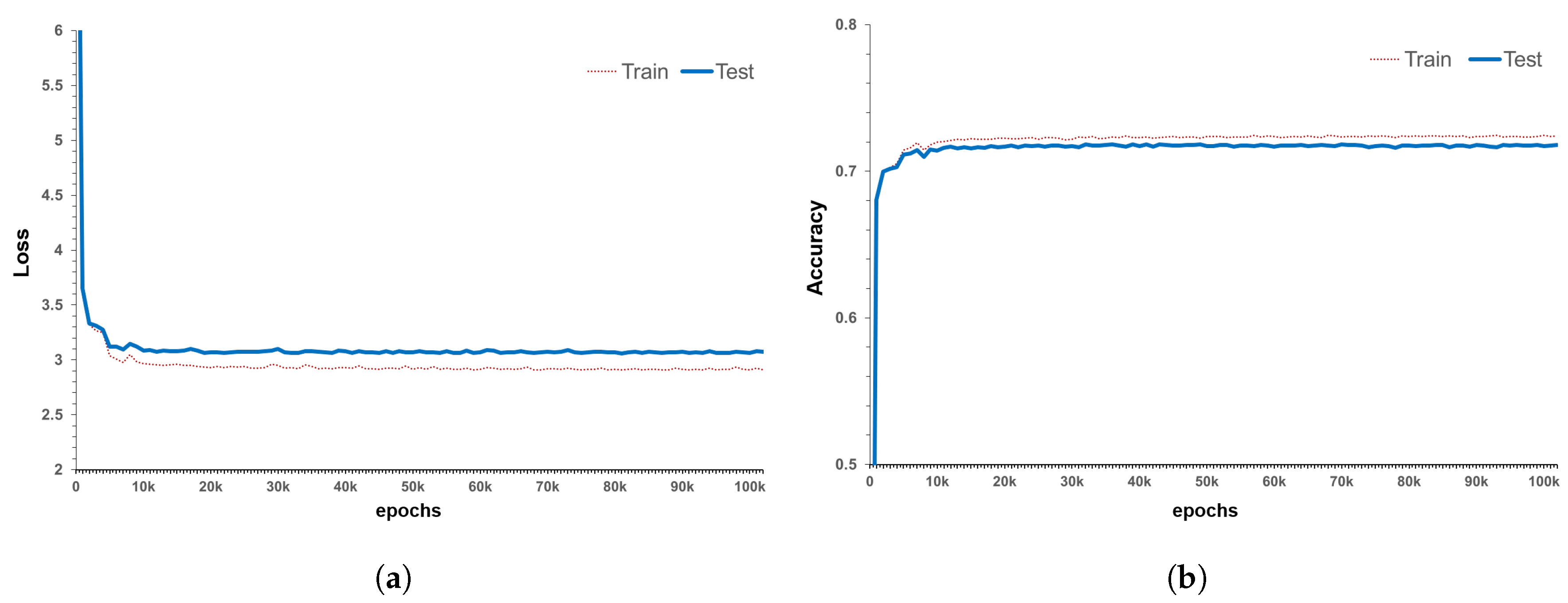
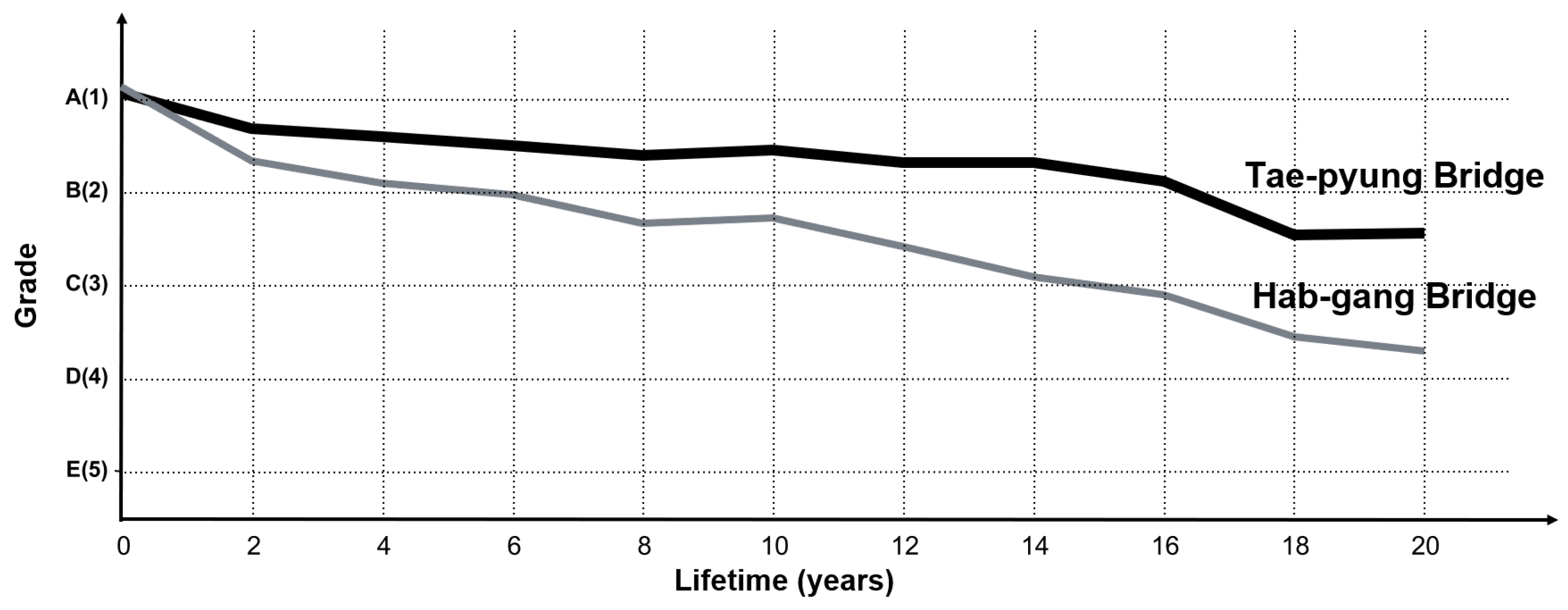
This paper presents a new performance degradation model of a concrete deck. As bridges are composed of various sorts of detailed member sets, the performance degradation model of each detailed member must be generated first. Thus, before developing a performance degradation model for bridges, this study used concrete deck inspection data from the bridge management system in Korea to develop a concrete deck performance degradation model. A deep-learning algorithm called LSTM was used to employ the inspection data, and the developed model is different from the existing models because it uses actual inspection data. Additionally, the developed model has the advantage that the same trained model can be applied to a new bridge. Label smoothing for converting the existing discrete labels into distribution patterns and the Layer Normalization method for effective training were used in the model generation. Using these techniques, the LSTM model was trained, training and testing results were compared, and the best model was selected. The selected model showed a distribution similarity of approximately 72% and exhibited training results almost similar to the test results. The developed model for the concrete deck was derived by estimating the probability of occurrence of five grades (A, B, C, D and E) for each sequence, and then, weighted averages of these calculated probabilities to express the grade. Then, the actual bridge design data was input to the developed model, and a performance degradation model of the concrete decks was created for each bridge. The predicted probability values showed similar results when compared with the actual bridge grade changes with multiple inspection data by Jin-Wui Bridge. In addition, as approximately 22 years of data were trained, the degradation model could be generated using only basic information on bridges that had not been actually inspected and those with little inspection data.

Our model is more objective because it utilizes the actual inspection data, unlike the existing bridge degradation models developed using material models and expert opinions. Thus, using these results, the model can be used as an objective index for decision-making, such as bridge inspection, maintenance and repair cycle, and estimation of the inspection cost. In the future, it will be possible to develop a model for a specific type of bridge, by combining various member models of the bridge. However, to upgrade the model, it is necessary to improve the current inspection method. In addition, the evaluation criteria for generating inspection and judgment errors should be revised.