Abstract
In the current low-carbon economy, the government has adopted carbon taxes and carbon trading policies to control the carbon emissions of manufacturers. As consumers become increasingly aware of low-carbon, some retailers have also started investing in low-carbon to shape their public image and increase their competitiveness to attract more customers. In this paper, the Stackelberg game method is utilized to solve the model, and the graphs are used to analyze the benefits of retailers’ low-carbon investment on the supply chain through numerical analysis. It is found that when the emission reduction cost coefficient of manufacturers is relatively low, manufacturers are willing to reduce carbon emissions. At this time, increasing carbon tax and the carbon emission permits price can effectively promote the emission reduction behavior of manufacturers, because it increases demand for products and the profit of manufacturers and retailers. However, when the emission reduction cost coefficient of the manufacturers is quite high, increasing carbon tax and carbon emission permits price cannot effectively promote the emission reduction behavior, because this situation of the emission reduction reduces the profit of manufacturers. The main contribution of this paper discovers that the green cost coefficient of retailers’ low-carbon investment will adjust the impact of the carbon tax and the carbon trading price on the profits of retailers and manufacturers which proves that retailers’ low-carbon investment is beneficial to the supply chain. When the emission reduction cost coefficient is high and the green cost coefficient is low, increasing the carbon tax or carbon emission permits price can increase the profit of manufacturers and retailers. Finally, we design a supply chain coordination of comprehensive sharing contact for retailers and manufacturers. The result shows that this contract has economic and environmental benefits, and that it is beneficial for the environment and economy of sustainable development.
1. Introduction
Rapid economic development has caused environmental problems. Awan et al. have put forward that the development of the industrial economy impacts the quality of human life and damages the natural environment. In particular, carbon emissions exacerbate global warming [1]. Environmental protection has become a great concern for the international community. In the reduction of carbon emissions and promoting the sustainable development of the global economy, countries worldwide generally adopt carbon tax and carbon trading as means through which to control carbon emissions [2]. Manufacturing companies directly affected by carbon emission reduction policies have to consider carbon emission reduction issues. The energy-saving and emission-reduction initiatives of manufacturing enterprises are mainly driven by government policies. At the same time, as consumers become increasingly aware of low-carbon, many manufacturers have already begun to produce environmentally friendly products to meet consumer needs. Some retailers have recently begun to introduce low-carbon investment in the packaging and distribution processes. For instance, in March 2017, JD.com developed a distribution system and set up a logistics packaging laboratory to promote the use of cleaner alternatives, such as environmentally friendly, biodegradable packaging [3]. With low-carbon investments, retailers can shape their public image, increase their reputation and attract more consumers that prefer low-carbon products. Walmart, the world’s largest retailer, wants to become a “low-carbon supermarket” and invest in environmentally friendly and energy-efficient stores, and has proposed a clean production solution for suppliers. Some scholars have studied the issues of energy conservation and emission reduction by manufacturers [4]. In fact, in the low-carbon economy, two forces exist in forcing enterprises to accomplish industrial upgrading, energy conservation, and emission reduction. One is government policy to manufacturers (carbon tax and carbon trading policies), and the other is market demand. As the side closest to the end demand, the retailer can feel the most change in consumer demand preferences and can most easily influence consumer demand preferences. Therefore, the retailers’ low-carbon investment can alter the supply chain.
Based on this phenomenon, some academic problems were generated as follows:
First, how does the retailer’s low-carbon investment affect supply chain profits under carbon tax and carbon trading policies? Second, how does the emission reduction cost coefficient of manufacturers affect the profits of manufacturers and retailers as the carbon tax and carbon emission price change? Third, how does the greenness coefficient affect the profits of manufacturers and retailers as the carbon tax and carbon emission price change? Fourth, how do manufacturers and retailers coordinate to increase the profits of the supply chain and improve the level of carbon emission reduction?
To answer the above questions, this study separately considers the consequences of whether the retailer makes low-carbon investments or not, as well as the existence condition and the corresponding equilibrium solution of manufacturer’s and retailer’s game equilibrium. The retailers making a low-carbon investment and those not are two separate scenarios, and these scenarios are analyzed under the two profits scenarios involving low-carbon consumer preferences, the emission reduction cost coefficient, green coefficient, carbon emission permit price, government-free carbon quotas, and carbon tax changes. Finally, a comprehensive sharing contract is designed for retailers with a low-carbon investment supply chain.
Most studies in the previous literature are of manufacturers’ emission reduction behavior or low-carbon investment behavior. In fact, retailers’ investment behavior can affect consumers’ demand for products. Few examples in the literature have studied the impact of retailers’ low-carbon investment on the demand and supply chain. This paper is different from the previous literature. From a quantitative perspective, in the context of carbon trading and carbon tax, the Stackelberg game method is used to study the impact of retailers’ low-carbon investment on the supply chain, and numerical analyses of the graphs are used to more intuitively explain the impact of parameters on the profits of manufacturers and retailers.
The main contributions of this study are as follows: (1) incorporating the retailer’s low-carbon investment decision into the contract design framework of the low-carbon supply chain increases the profits of manufacturers and retailers; (2) it is found that the greenness coefficient can adjust the impact of carbon tax and carbon emission rights prices on the profits of manufacturers and retailers; (3) this paper designs a “comprehensive sharing contract”, where retailers make a low-carbon investment under existing carbon tax and carbon trading policies. Notably, manufacturers increase emission-reduction levels through comprehensive sharing contracts. Thus, this contract has economic and environmental benefits. It is good for the environment and the economy of sustainable development.
2. Literature Review
In the current low-carbon economy, manufacturers choose carbon emission reductions. Moreover, as consumers become more aware of low-carbon, retailers make low-carbon investments. This research differs from the previous literature, in that this paper considers the retailers’ low-carbon investments and the coordination of retailers and manufacturers under existing carbon tax and carbon trading policies. This study mainly involves four literature streams: carbon tax and carbon trading policies, carbon emission reduction, retailer investment, and supply chain coordination.
2.1. Carbon Tax and Carbon Trading Policies
Carbon tax and carbon trading policy have a certain impact on economic development and the environment. Many scholars have studied and analyzed the impact of carbon tax and carbon trading policy. The environmental effect of carbon tax is unique to carbon tax as a tax policy to guide environmental protection, which contains certain social benefits. Baranzini et al. put forward that the environmental effects of carbon tax mainly include the following two aspects: First, carbon tax can effectively improve the energy structure, improve energy efficiency and guide the use of new energy. Second, carbon tax revenue can be earmarked as a financial subsidy to encourage the development of clean industries [4]. Wissema simulated the impact of carbon tax on the environment of Ireland through the CGE model, and concluded that the introduction of carbon tax can effectively improve the energy consumption structure of Ireland [5]. Lee also analyzed the impact of carbon tax and carbon emission trading rights on the economic effect of a country. The results of the study indicate that a country may have a negative impact on the economy when it only levies carbon taxes, but if carbon taxes and carbon emissions trading rights are levied at the same time, there is no negative impact. Therefore, in order to eliminate the negative economic effects of the carbon tax, he suggested that the two methods of carbon tax and carbon emissions trading rights be used simultaneously [6]. Rosic and Jammernegg put carbon tax and carbon trading into the dual-channel model considering the environmental impact of transportation, analyzed their impact on the transportation environment, and pointed out that in the case of carbon trading, enterprises can reduce the environmental impact of transportation without affecting the economic benefits. Therefore, carbon trading is better than carbon taxes [7]. Choi considered the influence of different forms of carbon emission tax on retailers’ choice of suppliers [8]. Lou used the Dynamic CGE Model to simulate and analyze the impact of carbon tax on China’s macro economy and carbon emissions [9]. Eichner et al. studied European Union-type carbon emission trading and the distributive effects of overlapping carbon taxes [10]. Fang et al. studied the impact of carbon trading on new energy. The results show that under certain conditions, carbon trading can promote the development of new energy, and mature carbon trading can effectively control carbon emissions and energy intensity [11]. Woo et al. investigated the impact of carbon trading on the real-time power market price in California. Researchers and policy makers generally agree that a carbon tax is the most effective mechanism to curb greenhouse gas emissions, but this tax has exacerbated inequality [12]. Fremstad et al. explored the impact of carbon taxes on inequality [13].
The above literature shows that there is abundant research on the impact of carbon tax and carbon trading policy on the social economy and environment. The research shows that although carbon tax can reduce carbon emissions and subsidize government finance, it may have a negative impact on social economic development. Carbon trading will also affect economic and environmental effects. However, as consumers’ awareness of low-carbon increases, carbon tax and carbon trading may have different impacts on the economy and environment. Considering consumers’ awareness of low-carbon in terms of demand assumption is a key factor in the modeling process of this paper.
2.2. Carbon Emission Reduction
There are a lot of researches on carbon emission reduction with different perspectives. Some scholars discuss strategies and factors for reducing carbon emissions. For instance, Awan et al. suggested that environmental management capabilities at production level have considerable value in addressing CO2 emissions and minimizing environmental pollution. It required a varied degree of competencies in the product life cycle, especially at the process and product levels, to ensure and improve pollution performance [14]. Many authors have studied cap-and-trade regulation among all carbon constraints, but some authors conducted their related research on carbon emission reduction. Moreover, some authors discuss carbon emission reductions under cap-and-trade regulation, but their focuses are different. For example, Yalabik and Fairchild established an economic analysis model to study carbon tax, consumer and competition on the impact of enterprise environmental innovation [15]. Luo et al. constructed the game models of the centralized decision-making, decentralized decision-making, and collaborative decision-making of supply chain members. They explored the game analysis of carbon emission reduction technology investment in the supply chain under carbon trading policy [16]. Chen et al. studied the problems faced by enterprises in terms of order acceptance and scheduling based on carbon emission reduction and electricity prices [17]. Zhang et al. explored the green innovation mode under carbon tax and innovation subsidies, and analyzed the influence of carbon tax and innovation subsidies on the manufacturer’s choice of green innovation mode. The results show that it is the carbon tax, but not the innovation subsidy, that remains effective in the later stage. It also discusses government policies intended to effectively promote the adoption of green innovations by manufacturers and reduce carbon emissions [18]. Bai et al. investigated the carbon emission reduction technologies of manufacturers under cap-and-trade regulation. The results showed that the profits of the supply chain can be improved, and that carbon emissions can be reduced under the decentralized scenario [19]. Zhang et al. discussed and compared the carbon emission rights price floor and revenue floor support schemes’ incentive effects on coal-fired power plants’ carbon emission reduction investment, considering random fluctuations of on-grid electricity volume and carbon prices. [20]. Ding et al. studied the impact of carbon tax and take-back legislation on enterprise production and carbon emission reduction decisions [21]. Du et al. pointed out that although many carbon emission regulations have been formulated to curb carbon emissions, some companies do not adopt low-carbon technologies because the extra cost is high. However, when consumers have a great preference for low-carbon products, manufacturers choose to reduce emissions by adopting low-carbon technologies [22]. In the study of carbon emission reduction, some papers have considered supply chain operation problems. For instance, Diabat et al. studied the location problem of multi-stage and multi-product enterprises under the carbon emission trading mechanism, and analyzed the impact of carbon trading prices on the cost and supply chain structure [23].
The above literature shows that, whether carbon emission reduction is carried out in the context of cap-and-trade regulation, carbon emission reduction strategy, or investment in low-carbon technology to produce products, most of the carbon emission reduction is mainly carried out by manufacturers, and few research retailers invest in emission reduction. In this paper, retailer investment in carbon emission reduction is the main research factor.
2.3. Retailer Investment
With an increasingly competitive market, retailers have begun to invest in various areas—such as advertising, packaging and transportation, radio frequency identification (RFID) technology and service—to attract customers and increase profit. Amrouche et al. investigated that retailers invested in advertising build a brand image [24]. Kesavan et al. studied the differences in retailer inventory investment behavior under macroeconomic shocks [25]. Moon et al. explored the investment strategic inventory of manufacturers and retailers, and the results showed that the investment efforts of manufacturers do not always persuade retailers to hold strategic inventory; however, when strategic inventory is used, the investment efforts of retailers can promote harmony. From a supply-chain coordination perspective, the retailer’s decision to carry out strategic inventory is disastrous, but benign for a fragmented supply chain [26]. Cao et al. explored the retailer’s advertising investment strategy. The results show that the retailer should set the retail price and order quantity at the monopolistic level, and adopt an “invest-all-or-none” advertising investment strategy for different market conditions. However, when market demand is random, the optimal strategy may fail [27]. Perdikaki et al. discussed how retailers determine the timing of service investment when product demand is uncertain and consumers are concerned about both price and service when choosing which retailer to buy from [28]. Yan et al. researched the financial services provided by retailers to cash-strapped suppliers and compared retailers’ financing schemes, e.g., loans and investments. It was found that both schemes brought additional value to retailers and suppliers with limited funds, providing a win–win situation [29]. Xia et al. pointed out that retailers have the opportunity to invest in store assistance to help consumers choose products and reduce product returns [30]. Tao et al. suggested that in the supply chain, retailers’ investment in radio frequency identification (RFID) technology is an effective method with which to solve inventory misplacement problems, and the results showed that the investment in RFID technology by retailers is more beneficial to both suppliers and retailers, and that end customers will also benefit more [31]. Hardgrave et al. investigated the effectiveness of investment in the use of RFID technology to reduce the inaccuracy of retail store inventory records through two different field experiments [32].
The above literature shows that many scholars study the investment of retailers in advertising, packaging and transportation, radio frequency identification (RFID) technology and service to increase profits. There is little research on retailers’ low-carbon investment. This paper studies the impact of retailers’ low-carbon investment on the supply chain, and considers the impact of consumer low-carbon awareness on demand in an incorporated supply chain coordination model. At the same time, the Stackelberg game method was used to solve the model and the graphs are used to analyze the benefits of retailers’ low-carbon investment on the supply chain through numerical analysis. However, Hardgrave et al. use two different field experiments for analyzing and investigating the effectiveness of investment in the use of RFID technology to reduce the inaccuracy of retail store inventories. These are two different research methods. We first modeled the theoretical hypothesis, then solved the model with the Stackelberg game, and finally used numerical analysis to draw graphs to verify the theoretical research results, while Hardgrave et al. verified and predicted the research results with field experimental data.
2.4. Supply Chain Coordination
In supply-chain mechanism design, various supply chain coordination mechanisms, such as wholesale price contract, repurchase contract, quantity flexible contract, and revenue sharing contract, were formed, and the efficiency and flexibility of these coordination mechanisms were analyzed [33,34,35,36,37]. The supply chain contract based on the entirely hypothetical information has realistic irrationality due to the existence of information asymmetry. Therefore, the focus of contract research was to promote information sharing within the supply chain and the optimization of the supply chain member operation strategy with incomplete information, and to achieve the Pareto improvement of the overall performance of the supply chain [38,39]. Many scholars have studied supply chain coordination from the perspectives of perishable goods [40], double-channel background [41], the existence of gray market and strategic consumers [42], and the large data environment [43]. To date, supply chain coordination has focused on reverse logistics, green supply chain and closed loop supply chain, and has tried to integrate environmental factors into supply chain coordination. In recent years, domestic and foreign scholars have gradually studied the coordination in low-carbon supply chains. Su et al. studied the coordination mechanism of green closed-loop supply chain based on the third party recycling, and analyzed the influence of centralized decision and decentralized decision on the returns and pricing strategies of each participant. Finally, an optimal cooperative mechanism decision model considering a cost-benefit sharing contract was designed [44]. Balan et al. provided guidance for the design of a low-carbon supply chain by modeling the overall carbon emissions of the supply chain [45]. Chaabane et al. [46] studied the design of sustainable supply chain under the carbon emission trading mechanism. Mohamad et al. explored the coordination mechanism of a supply chain under the European Union Emissions Trading Scheme, and established a second-level carbon emission supply chain model, which provided the possibility of supply chain emission reduction and cost reduction [47]. Shaw et al. studied the low-carbon clothing supply chain and optimized the carbon emission and cost of supply chains [48]. Tao et al. investigated optimal inventory control and supply chain coordination problems under the carbon footprint constraint [49].
Some terms are defined as follows: Supply chain coordination refers to a network consortium formed by two or more companies through company agreements or joint organizations in order to achieve certain strategic goals. Green supply chain is a modern management model that comprehensively considers the environmental impact and resource efficiency in the entire supply chain—that is, the green supply chain has the smallest negative environmental effect and the highest resource efficiency. Supply chain contract refers to the collaborative strategy of the upstream and downstream cooperative enterprises in the same supply chain, which replaces the hierarchical strategy with a global optimization strategy in the form of contracts to maximize the overall effect of the supply chain, such as through wholesale price contracts, repurchase contracts, quantity flexible contracts, and revenue sharing contracts. Closed-loop supply chain refers to the complete supply chain cycle of an enterprise from purchase to final sale, including the reverse logistics supported by product recovery and life cycle. It aims to reduce pollution emissions and residual waste.
From previous literature, the theoretical research on low-carbon supply chain management and coordination mainly focuses on the overall emission reduction and cost optimization or profit optimization of the supply chain under carbon emission restrictions. This paper considers the impact of consumer low-carbon awareness on demand in the incorporated supply chain coordination model.
In conclusion, different to the previous literature, this paper studies the impact of retailer investment on the supply chain in the context of carbon tax and carbon trading policies. Firstly, the increase in consumers’ awareness of low-carbon is considered, so the low-carbon investment of retailers will increase consumers’ demand, which is the key factor of this paper’s modeling. We then solve the model using the Stackelberg game, and finally use numerical analysis to draw graphs to verify the theoretical research results.
3. Assumption and Explanation of Symbols
Assumption 1.
This study considers a bilateral-monopoly two-level supply chain under carbon trading and carbon tax policies. The manufacturer determines the wholesale price w and emission reduction levelwhereas the retailer determines the retail price p and green level G. In addition, the manufacturer is the leader of the game. “Green level” is the impact level of the entire production and operation of the enterprise on the environment and the “green level information” that is transferred from the enterprise to society. “Green level” is related to the low-carbon investment strategy of the enterprise. In this case, this paper assumes that the retailer’s low-carbon investment , of whichis greenness coefficient, and that a large greenness coefficient means a great need to invest to reach a certain green level. It is common to use the form of quadratic function to indicate the cost pattern of this kind, which can be seen in examples from the existing literature including Chintagunta et al., Liu et al. and Zhou et al. [50,51,52].
Assumption 2.
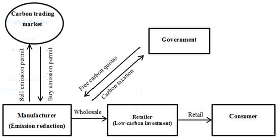
The government charges the manufacturer carbon taxper unit of carbon emission according to the actual carbon emission of the manufacturer, and allocates a certain amount of free carbon quotas Eg to the manufacturer. The manufacturer could buy or sell carbon emission permits in the carbon trading market, whereas the retailer does not participate in carbon emission reduction or carbon trading, and does not need to pay carbon tax. The low-carbon supply chain system is shown as Figure 1.
Figure 1.
Low-carbon supply chain system.
Assumption 3.
Consumers have low-carbon preference so that both manufacturer’s emission reduction and retailer’s low-carbon investment would stimulate demand.
Assumption 4.
The price of carbon emission permitsis determined by the carbon trading market and it is an exogenous variable.
Assumption 5.
This model ignores the production cost.
Assumption 6.
The manufacturer always reduces emission at first and then buys emission permits from carbon trading market if it does not come up to the emission reduction standard made by government.
Assumption 7.
The low-carbon investment of retailer includes biodegradable packaging and low-carbon distribution processes.
The major parameters and notations are listed in Table 1 as follows.

Table 1.
The major parameters and notations.
4. Modeling
4.1. The Retailer Does Not Make a Low-Carbon Investment
According to findings in the literature [51,53,54], we assume that the market demand of low-carbon products is sensitive to consumers’ low-carbon preference and price-influencing demand. It assumes the market demand as follows:
Carbon emission permits that the manufacturer should sell or buy in carbon trading market as follows:
Then, the profit of the retailer is calculated as follows:
where superscript n represents the situation that the retailer does not make a low-carbon investment.
The profit of the manufacturer is made up of four parts: sales income , manufacturer’s income or payout related to price of carbon emission rights peEt, emission reduction cost , and expenditure on carbon tax. Thus, the profit of the manufacturer is as follows:
Proposition 1.
The unique game equilibrium exists so that the profits of the manufacturer and the retailer can reach the maximum ifand, and the game equilibrium is as follows:
The profits of the manufacturer and the retailer are calculated as follows:
Proof—see Appendix A.
Proposition 2.
When the retailer does not make a low-carbon investment, the change laws of the retailer’s profitas emission reduction cost coefficient, consumer’s low-carbon preference, price of carbon emission permits pe,and carbon taxchange are as follows:
- (i)
- decreases in .
- (ii)
- increases in.
- (iii)
- If, thenincreases in pe. if, thendecreases in pe.
- (iv)
- If, thenincreases in. if, thendecreases in.
Proof—see Appendix A.
Proposition 3.
When the retailer does not make a low-carbon investment, the change laws of the manufacturer’s profitas emission reduction cost coefficient, consumer’s low-carbon preference, free carbon quotas Eg, price of carbon emission permits pe,and carbon taxchange are asfollows:
- (i)
- decreases in.
- (ii)
- increases in.
- (iii)
- increases in Eg.
- (iv)
- If, orand, thenincreases in pe. ifand, thendecreases in pe.
- (v)
- If, thenincreases in. if, thendecreases in.
Proof—see Appendix A.
According to Propositions 2 and 3, the following corollaries are obtained:
Corollary 1.
The profits of manufacturers and retailers decrease with the increasing manufacturer’s emission reduction cost coefficient, suggesting that the retailer’s profit is relevant to the manufacturer’s carbon emission reduction behavior. Hence, the cooperation between retailers and manufacturers can decrease the emission reduction cost coefficient. This decrease is beneficial for the manufacturer and the retailer, and it will provide a theoretical basis for cooperation to reduce emissions.
Corollary 2.
The profits of manufacturers and retailers increase with the increase in consumers’ low-carbon preference. Thus, the manufacturer and the retailer should make efforts towards energy conservation, emission reduction, and low-carbon investment.
Corollary 3.
Carbon tax and carbon emission permit price indirectly affect the retailer’s profit by affecting the emission reduction behavior of the manufacturer. When the manufacturer’s carbon emission reduction in cost coefficient is relatively low, the retailer’s profit increases as the prices of carbon emission rights and carbon tax increase, because increasing the prices of carbon emission permits and carbon tax can effectively promote the emission reduction behavior of the manufacturer. When the manufacturer’s carbon emission reduction in cost coefficient is relatively high, the retailer’s profits decrease with the increasing price of carbon emission permits and carbon tax, because increasing the carbon emission permits price and carbon tax cannot effectively promote the emission reduction behavior of the manufacturer. Hence, manufacturers are reluctant to invest in carbon reduction because the cost of carbon reduction to the manufacturer is too high. Increasing the emission reduction cost makes manufacturers transfer a part of its cost to the retailer by increasing the wholesale price.
Corollary 4.
The carbon tax and carbon emission permits price directly affect the profit of the manufacturer; however, because the manufacturer can obtain a free carbon allowance from the government, when the carbon emission reduction in cost coefficient is high, and as long as the free carbon allowance is large, the profit of the manufacturer will increase as the carbon emission permit price increases.
4.2. Retailer Makes a Low-Carbon Investment
The increase in consumers’ awareness of low-carbon is considered, so the low-carbon investment of retailers will increase consumers’ demand, and the market demand is assumed as follows:
Carbon emission permits that the manufacturer should sell or buy in the carbon trading market are illustrated follows:
This time, the retailer has low-carbon investment . Thus, its profit is calculated as follows:
The profit of the manufacturer is shown as follows:
Proposition 4.
The unique game equilibrium exists so that the profits of the two could reach the maximum, if,, and, and the game equilibrium is as follows:
Proposition 5.
When the retailer makes a low-carbon investment, the change laws of retailer’s profit as green level coefficient , emission reduction cost coefficient , consumer’s low-carbon preference , price of carbon emission rights pe, and carbon tax t change are as follows:
- (i)
- decreases in.
- (ii)
- decreases in.
- (iii)
- increases in.
- (iv)
- If, orand, thenincreases in pe.Ifand, thendecreases in pe.
- (v)
- If, orand, theincreases in.Ifand, thendecreases in.
Proof—see Appendix A.
Proposition 6.
When the retailer makes a low-carbon investment, the change laws of manufacturer’s profitas emission reduction cost coefficient , consumer’s low-carbon preference , free carbon quotas Eg, emission permits price pe, and carbon tax change are as follows:
- (i)
- decreases in.
- (ii)
- increases in.
- (iii)
- increases in Eg.
- (iv)
- If, orand, or,and, thenincreases in pe, if,and, thendecreases in pe.
- (v)
- If, orand, thenincreases in;ifand, thendecreases in.
Proof—see Appendix A.
According to Propositions 5 and 6, the following corollaries are obtained:
Corollary 5.
Following the retailer’s low-carbon investment, the cost coefficient, low-carbon consumer preferences and government free carbon quotas on the influence of the retailer’s and manufacturer’s profits trends remain the same. Moreover, the profits of retailers and manufacturers decrease with the increase in the emission reduction cost coefficient. The profits of manufacturers and retailers increase with the increase in the consumer’s low-carbon preference. Furthermore, the manufacturer’s profit increases with the increase in the government free carbon quota.
Corollary 6.
The greenness coefficient can adjust the impact of carbon tax and carbon emission permit price on the profits of manufacturers and retailers. Previously, the retailer has not carried out low-carbon investment, and the profits of manufacturers and retailers have been negatively correlated with the carbon tax and carbon emission permits price. After the low-carbon investment, when the greenness coefficient is low, the profits of manufacturers and retailers can be positively correlated with the carbon tax and carbon emission price. This condition indicates that under existing carbon tax and carbon trading policies, when the green factor is low, retailers are then willing to invest in low-carbon; hence, the retailer’s low-carbon investment will have a huge impact on the entire supply chain, thus causing different changes for the entire supply chain.
Proposition 7.
When carbon trading and carbon tax coexist and the game equilibrium exists, low-carbon investment is good for retailers and manufacturers. Hence,and.
Proof.
When the game equilibrium exists, regardless of whether the retailer makes a low-carbon investment or not, there are , , and . Before and after the low-carbon investment, the profits margins of the two are.
and , respectively. The known conditions can deduce that and , and given that , there is when . □
According to Proposition 7, the following corollaries are obtained:
Corollary 7.
When carbon trading and carbon tax coexist, and the game equilibrium exists regardless of whether or not the retailer makes low-carbon investments, the retailer’s low-carbon investment will increase the profits of manufacturers and retailers. Therefore, the retailer should make low-carbon investments.
Corollary 8.
When carbon trading and taxes coexist, the manufacturer reduces carbon emissions; at the same time, and the retailers’ low-carbon investment will be a win–win situation. Moreover, the retailers’ low-carbon investment will have a positive impact on the social environment.
Under carbon tax and carbon trading policies, the supply chain has a double marginal effect when the retailer makes a low-carbon investment and the manufacturer reduces carbon emissions. Moreover, decentralized decision making will decrease the low-carbon investment level and carbon emission reduction level to lower than the overall optimal level. Therefore, the supply chain coordination problem for retailers to make low-carbon investment will be discussed.
4.3. Coordination of Supply Chain When the Retailer Makes a Low-Carbon Investment
4.3.1. Centralized Decision of Supply Chain
The total profit of supply chain is as follows:
Proposition 8.
The unique game equilibrium exists so that the total profit of supply chain can reach the maximum if,and, and the game equilibrium is as follows:
The total profit of supply chain is as follows:
4.3.2. Centralized Decision of Supply Chain
It was found that two-part tariff and cost-sharing contracts cannot coordinate the supply chain when it contains manufacturer-quality and retailer-marketing efforts, and those efforts would increase demand [55]. Our model is similar to their model to a certain extent, in that the manufacturer invests in emission reductions for products, the retailer invests in low-carbon construction, and both sides increase demand. However, this study simultaneously involves carbon trading and carbon tax. Thus, the supply chain operations would be complex. This condition can prove that traditional contracts, such as two-part tariff and cost-sharing, will not be able to coordinate the supply chain studied in this work. Therefore, a novel contract is designed in this paper to coordinate the supply chain when the retailer makes a low-carbon investment under existing carbon tax and carbon trading policies. The sum of the profits of the two parties is equal to the profits when the decision-making situation is concentrated. The design idea of the contract is to let the manufacturers and retailers carry out comprehensive revenue sharing and cost sharing, which is called a comprehensive shared contract. The specific design is as follows:
The manufacturer sets the wholesale price β1p and shares a part of low-carbon investment of the retailer. Meanwhile, the retailer shares a part of the emission reduction cost and carbon tax and shares a part of the revenue or cost related to emission permits. Under this contract, the profits of the retailer and manufacturer are shown as follows:
Proposition 9.
The supply chain could be coordinated when , and.
Proof of Proposition 9.
When and , the profits of the retailer and manufacturer are as follows:
The game between the retailer and the manufacturer is a Stackelberg game. Thus, an inverse solution is adopted.
Substituting Equations (10) and (11) into Equation (27), Equation (29) could be obtained:
Taking the first derivative of Equation (29) with respect to and G, Equation (30) and (31) could be obtained:
In addition, the Hessian matrix is:
The matrix needs to be negatively definite. Thus, there is maximum of Πr exists. From and , Equations (32) and (33) could be obtains:
Substituting Equations (10), (11), (32) and (33) into Equation (28) and taking the first derivative of with respect to λ, Equation (34) could be obtained:
From , can be obtained. Then, the maximum of exists. In addition, from , can be obtained. Substituting into Equations (32) and (33),
and can be obtained. Thus, there are , , and .
Substituting , and into the profits functions of the retailer and manufacturer, and can be obtained. By this time, there is . In other words, the supply chain is coordinated.
In addition, this contract has to meet the participation constraint of the retailer and manufacturer. Then, and must be met. Solving these equations, can be obtained. □
Proposition 10.
Through coordination by comprehensive sharing contract, the manufacturer would increase in emission reduction level, and the retailer would increase in low-carbon investment level.
Proof of Proposition 10.
, , and there are , , and . Therefore, and . □
According to Propositions 8–10, the following corollary is obtained:
Corollary 8.
In the current low-carbon economy, an enterprise should deepen the cooperation with its upstream and downstream enterprises if it wants to increase in profits. Complete revenue sharing and cost sharing could reduce double marginalization to a maximum degree, and increase in the profits for the enterprise and even the entire supply chain. This kind of cooperation could increase in the manufacturer’s emission reduction and the retailer’s low-carbon investment level. Thus, this contract not only has economic benefits but also has social environment benefits. It is good for the environment and economic of sustainable development.
5. Numerical Analysis
To analyze the impact of carbon emission reduction coefficient, consumers’ low-carbon preference level, green degree, carbon emission trading price, and carbon tax on the profits of manufacturers and retailers and emission reduction level of the manufacturer, some numerical examples are given below to illustrate the results of this study. Based on all the constraints of the model, , and .
Let .
5.1. Retailer Does Not Make a Low-Carbon Investment
- (1)
- The figure is drawn by numerical analysis. It is found that as shown in Figure 2 and Figure 3, increasing the carbon emission permits price and carbon tax can increase the retailer’s profit when the cost coefficient of carbon emission reduction is low. However, when the cost coefficient of carbon emission reduction is high, increasing the carbon emission permits price and carbon tax can decrease the retailer’s profit. These observations suggest that the retailer’s profit and the manufacturer’s carbon aemission reduction behavior are relevant. Hence, cooperation between retailers and manufacturers can lower the emission reduction cost coefficient, and thus benefit manufacturers and retailers in providing the theoretical basis that cooperation reduces emissions. Proposition 2 of (iii) and (iv) is thus verified.
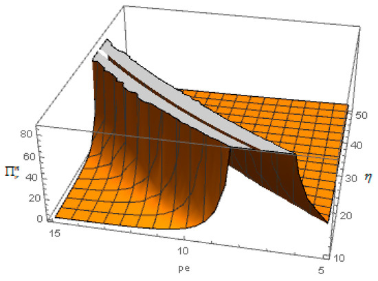 Figure 2. Effect of carbon emission permits price on the retailer’s profit.
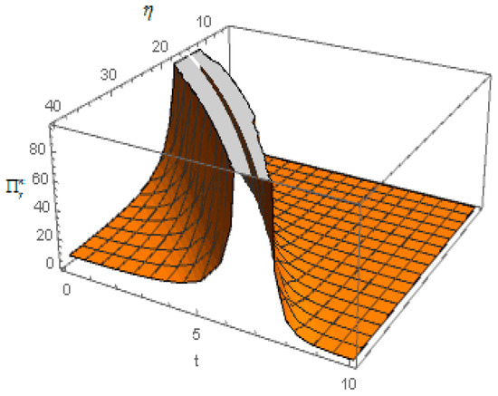 Figure 3. Effect of carbon tax on the retailer’s profit .
 - (2)
- The figure is drawn by numerical analysis. It is found that Figure 4 demonstrates that when the cost coefficient of carbon emissions reduction is low, or when the carbon emission reduction cost coefficient is high and the free carbon quota of the government is high enough, the carbon emission permits price promotes carbon emission reduction by the manufacturer. Proposition 3 of (iv) is thus verified. Figure 5 shows that under case 1, when the cost coefficient of carbon emissions reduction is low, the carbon tax can promote carbon emission reduction by the manufacturer. Proposition 3 of (v) is thus verified.
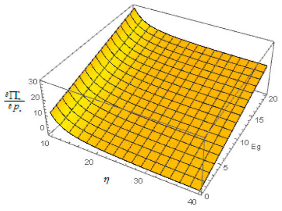 Figure 4. Effect of carbon emission permits price on the manufacturer’s profit .
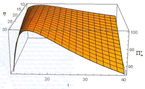 Figure 5. Effect of carbon tax on the manufacturer’s profit .
5.2. Retailer Makes a Low-Carbon Investment
- (1)
- The figure is drawn by numerical analysis. It is found that Figure 6 demonstrates that under case 2, when the cost coefficient of carbon emission reduction is low, or when the cost coefficient of carbon emission reduction is high and the green level coefficient is low, increasing the carbon emission permits price can increase the retailer’s profit. Moreover, when the cost coefficient of carbon emission reduction is high and the green level coefficient is high, increasing the carbon emission permits price can decrease the retailer’s profit. Proposition 5 of (iv) is thus verified.
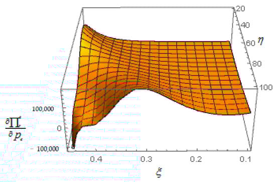 Figure 6. Effect of carbon permits price on the retailer’s profit .
 - (2)
- The figure is drawn by numerical analysis. It is found that Figure 7 demonstrates that under case 2, when the cost coefficient of carbon emission reduction is low, or when the carbon emission reduction cost coefficient is high and green level coefficient is low, increasing the carbon tax can increase the retailer’s profit. Moreover, when the cost coefficient of carbon emission reduction is high and the green level coefficient is high, increasing carbon tax decreases the retailer’s profit. Proposition 5 of (v) is thus verified.
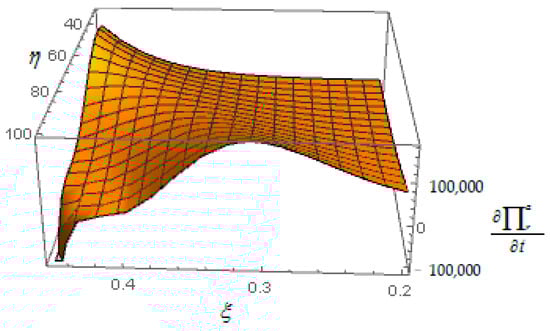 Figure 7. Effect of tax on the retailer’s profit .
 - (3)
- The figure is drawn by numerical analysis. It is found that Figure 8a,b demonstrate that under case 2, when the cost coefficient of carbon emission reduction is low, or when the cost coefficient of carbon emission reduction cost is high and the green level coefficient is low, or when the cost coefficient of carbon emission reduction is high, the green level coefficient is high and the free carbon quota of the government is high, the carbon emission permits price can increase the profit of manufacturers. Moreover, when the cost coefficient of carbon emission reduction is high and the green level coefficient is high, increasing the carbon emission permits price can decrease the profit of manufacturers. Proposition 6 of (iv) is thus verified.
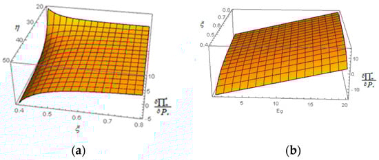 Figure 8. (a) Effect of carbon emission permits price on the manufacturer’s profit ; (b) Effect of carbon emission permits price on the manufacturer’s profit .
 - (4)
- The figure is drawn by numerical analysis. It is found that Figure 9 demonstrates that under case 2, when the cost coefficient of carbon emission reduction is low, or when the carbon emission reduction cost coefficient is high and the green level coefficient is low, increasing the carbon tax can increase the profit of manufacturers. Moreover, when the cost coefficient of carbon emission reduction is high and the green level coefficient is high, increasing the carbon tax can decrease the profit of the manufacturer. Proposition 6 of (iv) is thus verified.
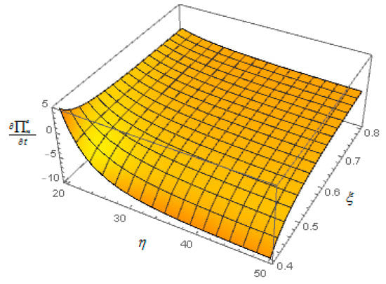 Figure 9. Effect of carbon tax on the manufacturer’s profit .
6. Discussion
After numerical analysis, some conclusions are as follows:
When the emission reduction cost coefficient of the manufacturer is relatively low, the manufacturer is willing to reduce carbon emissions. Increasing the carbon tax and carbon emission permits price can effectively promote the emission reduction behavior of the manufacturer. Previous literature has also demonstrated that a carbon tax can reduce carbon emissions [4,5,9,56]. Thus, the profit of the retailer increases with the increase in carbon tax and carbon emission permits price. When emission reduction cost coefficient is relatively high, the manufacturer may be not willing to reduce carbon emissions. In addition, increasing the carbon tax and carbon emission permits price cannot effectively promote the emission reduction behavior of the manufacturer; moreover, the profit of the retailer decreases as the carbon tax and carbon emission permits price increase, because when emission reduction cost coefficient is high, the manufacturer will pass on a part of the cost to the retailer by increasing the wholesale price. This effect is due to the increase in emission reduction cost coefficient, which decreases the profit of the retailer. It is clear that the investment coefficient of carbon reduction is a major obstacle to increasing the rate of carbon reduction as well as supply chain profit. To address this issue, the supply chain should give thought to utilizing external expertise in carbon reduction to take advantage of the appropriate technology. Shabbir et al. and Yadoo et al. have investigated using carbon reduction technology to reduce carbon emissions [57,58].
The greenness coefficient can adjust the impact of carbon tax and carbon emission price on the profits of manufacturers and retailers. When the retailers make low-carbon investments, the profits of manufacturers and retailers are negatively correlated with carbon tax and carbon emission price. When the retailers make low-carbon investments and greenness coefficient is low, the profit of manufacturers and retailers is positively correlated with carbon tax and carbon emission price. When the greenness coefficient is low, as consumers become increasingly aware of low-carbon, the retailers are willing to make low-carbon investments, and the low-carbon investment of retailers greatly affects the entire supply chain and causes different changes. Yang et al. and Bai et al. highlight the importance of low-carbon environmental awareness to the supply chain [59,60].
7. Conclusions
The purpose of this paper is to explore the impact of retailers’ low-carbon investment on the supply chain in the context of carbon tax and carbon trading policies. Firstly, the increase in consumers’ awareness of low-carbon is considered, so the low-carbon investment of retailers will increase consumers’ demand, which is a key factor of this paper’s modeling. Based on this framework, we study two cases to explore the impact of retailers’ low-carbon investment on the supply chain: (i) The retailer does not make a low-carbon investment. (ii) The retailer makes a low-carbon investment. After deriving the equilibrium solutions for two cases, we obtain novel insights into the equilibrium with respect to retailers’ low-carbon investment. Firstly, through comparative analysis, it can be seen that the profits of both sides of retailers are higher when they make low-carbon investments than when they do not make low-carbon investments. Therefore, under the policies of carbon trading and carbon tax, the low-carbon investment of retailers is very beneficial to the supply chain. Firstly, through comparative analysis, it can be seen that when the retailer makes low-carbon investments, the profits of retailer and manufacturer are higher than their profits when they do not make low-carbon investments. Therefore, under the policies of carbon trading and carbon tax, the low-carbon investment of retailers is very beneficial to the supply chain. It is found that the greenness coefficient will adjust the impact of carbon tax and carbon trading price on the profits of retailers and manufacturers. So when the greenness coefficient of retailers and emission reduction cost coefficient of manufacturers are high, the government should implement a series of policies to reduce the emission reduction cost coefficient of the manufacturer and greenness coefficient of the retailer so that it increases the profit of the entire supply chain and makes the manufacturer reduce carbon emissions for environmental benefit. At last, we design a supply chain coordination of comprehensive sharing contact for the retailers and manufacturers; the result shows that this contract has economic and environmental benefits. It is good for the environment as well as the economy of sustainable development.
In the face of global warming, low-carbon behavior is the responsibility and obligation for every country, every company, and every consumer. As consumers’ awareness of low-carbon environmental protection increases, consumers increase demand for low-carbon products and enhance the recognition of low-carbon concept of enterprises. Through the analysis of this paper, we have obtained the above conclusions. We provide some suggestions and management implications for the government and enterprises as follows:
7.1. Government Optimal Policy
In summary, the government should make some policies for manufacturers and retailers, on the one hand, using carbon tax and carbon trading policies to promote manufacturers to reduce emissions; on the other hand, subsidies can be made when the green cost coefficient of retailers is high, and the government can encourage the retailer to invest in low-carbon. When the carbon emission reduction cost coefficient is high, the government encourages manufacturers to exploit new low-cost carbon emission reduction technologies with some incentives or preferential policies for manufacturers. The government is a promoter of low-carbon technology innovation. Policy incentives and support have an irreplaceable role in promoting low-carbon technology innovation and commercial application. The government should formulate some preferential policies and protective measures for enterprises developing low-carbon technologies, such as the government’s tax deduction policy for enterprises developing low-carbon technologies, the government can invest in demonstration projects for low-carbon technology development, and implement intellectual property protection. The government can use tax deduction policy or subsidies to encourage manufacturers and retailers to utilize low-carbon technologies. Carbon emission reduction subsidies are provided for these manufacturers with the high cost of emission reduction, such as subsidies for the construction and renovation of environmental protection facilities and replacement of emission reduction equipment.
7.2. Management Implications for the Manufacturer Enterprise
In a low-carbon economic environment, consumers ‘low-carbon preference is the compass of production and development of enterprises. In order to meet consumers’ low-carbon preference need, enterprises develop and produce low-carbon environmentally friendly products, and strive to reduce carbon dioxide emissions from the production line to establish enterprises low-carbon concept image. The logo on the product indicates the low-carbon concept, reminds consumers to pay attention to the low-carbon and environmental protection issues in the use process, to guide consumers to low-carbon consumption behavior, so as to better establish the low-carbon concept of enterprises and attract more consumers to buy products. In the stage of product discarding and recycling, recycling is adopted, so that the company truly implements the low-carbon concept, and lays a foundation for the sustainable development of enterprises.
7.3. Management Implications for the Retail Enterprise
Through the analysis of this paper, it can be concluded that retailers’ low-carbon investment behavior can affect the whole supply chain, because retailers are the closest to consumers, and retailers gain a better understanding of consumers’ low-carbon preference compared with manufacturers. Meanwhile, retailers’ low-carbon investments will also affect consumers’ choices. Retailers should implement low-carbon measures in the provision of goods and services, commodity distribution, store facilities, store operation and waste disposal, so as to establish a good enterprise low-carbon concept and attract more consumers. For instance, store equipment should be energy-saving and low-carbon, and waste should be dealt with and reused in a low-carbon way. The retail enterprises carry out low-carbon distribution based on the application of new technologies and deliver low-carbon concepts. The retail enterprises strengthen the linkage and cooperation with manufacturers to build a true low-carbon supply chain. The retail enterprises deliver low-carbon concepts to consumers and guide consumers to low-carbon behavior, and, in turn, win more consumers.
7.4. Future Research Direction
Further research can be conducted in the future. Firstly, this study only considers a two-stage supply chain consisting of manufacturers and retailers. Future work should consider a multistage complex supply chain with multiple manufacturers and retailers. Secondly, future research can add competitive factors in supply chain.
Author Contributions
Professional guidance, Y.Z.; research design, writing of paper, F.Z., C.Y. All authors have read and agreed to the published version of the manuscript.
Funding
The research is supported by Chinese National Funding of Social Science (Grant No. 71471178).
Conflicts of Interest
The authors declare no conflict of interest.
Appendix A
Proof of Proposition 1.
The game between the retailer and the manufacturer is a Stackelberg game, so we adopt an inverse solution.
Substituting Equation (1) into Equation (3), the profit of the retailer can be obtained:
Taking the first derivative of with respect to , it can be obtained:
Afterwards, there is , so when , the profit of the retailer reaches the maximum, and it can be obtained:
Substituting Equations (1), (2) and (A2) into Equation (4), the profit of the manufacturer can be obtained:
Taking the first derivative of with respect to and we obtain:
and the Hessian matrix is:
The matrix needs to be negative definite, so there is , and then the maximum of exists. From and , it can be obtained:
substituting them into Equation (A2), we obtain: .
Substituting , , and into Equation (A1) and (A4), we obtain:
Substituting and into Equation (1), we obtain , and we deduce from that . □
Proof of Proposition 2.
There are , .
- (1)
- , so there are and decreases in .
- (2)
- , so there are and increases in .
- (3)
- , and , so when , there are and increases in . When , there is , and decreases in .
- (4)
- , so when , there are and increases in . When , there are and decreases in .
□
Proof of Proposition 3.
There are , .
- (1)
- , so decreases in .
- (2)
- , so increases in .
- (3)
- , so increases in .
- (4)
- , and , so when , is always held, while when and , there is . When and , there is .
- (5)
- , so when , there is . when , there is
□
Proof of Proposition 4.
The game between the retailer and the manufacturer is a Stackelberg game, so we adopt an inverse solution.
Substituting Equation (10) into Equation (11), the profit of the retailer can be obtained:
Taking the first derivative of with respect to and , we obtain:
and the Hessian matrix is:
The matrix needs to be negative definite, so there is , and then the maximum of exists. From and , it can be obtained:
Substituting Equations (10), (11), (A10) and (A11) into Equation (13), the profits of manufacturer can be obtained:
Taking the first derivative of with respect to and , we obtain:
and the Hessian matrix is:
According to the preceding proofs, there is . It can be deduced from negative definite of the matrix that , and then the maximum of exists. From and , there are and . Substituting them into Equation (A10) and (A11), the following can be obtained: and .
Substituting , , and into Equation (A7) and (A12), we obtain: and .
Substituting , and into Equation (10), we obtain:
. From , there is . Since , we choose among and . □
Proof of Proposition 5.
There are , and .
- (1)
- , and , so when , is always held, then there is , and decreases in .
- (2)
- , since , there is , and decreases in .
- (3)
- , since , there is , and increases in .
- (4)
- , when , is always held. There is , so when , is always held, while when , there is , so when and , there is , and when and , there is .
- (5)
- , it is the same with , so when , or and , there is . When and , there is . □
Proof of Proposition 6.
We have , and .
- (1)
- , so decreases in .
- (2)
- , so increases in .
- (3)
- , so increases in .
- (4)
- , when , is always held.Where is , so when , is always held. When , there is , so when and , is always held. While when , and , there is , and when , and , there is .
- (5)
- , when , is always held, so when , is always held. While when and , we have , and when and , there is .
□
Proof of Proposition 8.
Substituting Equation (10) and (11) into Equation (20), the following can be obtained:
Taking the first derivative of with respect to , , and , the following can be obtained:
and the Hessian matrix is:
The matrix needs to be negative definite, so we have and , then the maximum of exists. From , and , the following can be obtained: , and .
Substituting them into Equation (A15), the following can be obtained: .
Substituting , and into Equation (10), the following can be obtained: . From , there is . □
References
- Awan, U.; Kraslawski, A.; Huiskonen, J. Governing Interfirm Relationships for Social Sustainability: The Relationship between Governance Mechanisms, Sustainable Collaboration, and Cultural Intelligence. Sustainability 2018, 10, 4473. [Google Scholar] [CrossRef]
- Wu, P.; Jin, Y.; Shi, Y.J.; Shu, H. The impact of carbon emission costs on manufacturers’ production and location decision. Int. J. Prod. Econ. 2017, 193, 193–206. [Google Scholar] [CrossRef]
- Aifan. JD.COM’s Development on Carton Transform System. Available online: http://www.techweb.com.cn/internet/2017-03-21/2503052.shtml (accessed on 23 April 2020).
- Baranzini, A.; Goldemberg, J.; Speck, S. A future for carbon taxes. Ecol. Econ. 2000, 32, 395–412. [Google Scholar] [CrossRef]
- Wissema, W.; Dellink, R. AGE analysis of the impact of a carbon energy tax on the Irish economy. Ecol. Econ. 2007, 61, 671–683. [Google Scholar] [CrossRef]
- Lee, C.F.; Lin, S.J.; Lewis, C. Analysis of the impacts of combining carbon taxation and emission trading on different industry sectors. Energy Policy 2008, 36, 722–729. [Google Scholar] [CrossRef]
- Rosič, H.; Jammernegg, W. The economic and environmental performance of dual sourcing: A newsvendor approach. Int. J. Prod. Econ. 2013, 143, 109–119. [Google Scholar] [CrossRef]
- Choi, T.-M. Optimal apparel supplier selection with forecast updates under carbon emission taxation scheme. Comput. Oper. Res. 2013, 40, 2646–2655. [Google Scholar] [CrossRef]
- Lou, F. Simulation study on the carbon tax impact on China’s macro economy and carbon emission reduction. J. Quant. Tech. Econ. 2014, 10, 84–109. [Google Scholar]
- Eichner, T.; Pethig, R.; Pethig, R. EU-type carbon emissions trade and the distributional impact of overlapping emissions taxes. J. Regul. Econ. 2010, 37, 287–315. [Google Scholar] [CrossRef][Green Version]
- Fang, G.; Lu, L.; Tian, L.; Yin, H. Research on the influence mechanism of carbon trading on new energy—A case study of ESER system for China. Phys. A Stat. Mech. Appl. 2020, 545, 123572. [Google Scholar]
- Woo, C.; Chen, Y.; Zarnikau, J.; Olson, A.; Moore, J.; Ho, T. Carbon trading’s impact on California’s real-time electricity market prices. Energy 2018, 159, 579–587. [Google Scholar] [CrossRef]
- Fremstad, A.; Paul, M. The Impact of a Carbon Tax on Inequality. Ecol. Econ. 2019, 163, 88–97. [Google Scholar] [CrossRef]
- Awan, U.; Kraslawski, A.; Huiskonen, J. Progress from Blue to the Green World: Multilevel Governance for Pollution Prevention Planning and Sustainability. In Handbook of Environmental Materials Management; Springer Science and Business Media LLC: Berlin/Heidelberg, Germany, 2019; pp. 1–22. [Google Scholar]
- Yalabik, B.; Fairchild, R.J. Customer, regulatory, and competitive pressure as drivers of environmental innovation. Int. J. Prod. Econ. 2011, 131, 519–527. [Google Scholar] [CrossRef]
- Luo, R.L.; Fang, T.J.; Xia, H. The game analysis of carbon reduction technology investment on supply chain under carbon cap-and-trade rules. Chin. J. Manag. Sci. 2014, 22, 44–53. [Google Scholar]
- Chen, S.-H.; Liou, Y.-C.; Chen, Y.-H.; Wang, K.-C. Order Acceptance and Scheduling Problem with Carbon Emission Reduction and Electricity Tariffs on a Single Machine. Sustainability 2019, 11, 5432. [Google Scholar] [CrossRef]
- Zhang, S.; Yu, Y.; Zhu, Q.; Qiu, C.; Tian, A. Green Innovation Mode under Carbon Tax and Innovation Subsidy: An Evolutionary Game Analysis for Portfolio Policies. Sustainability 2020, 12, 1385. [Google Scholar] [CrossRef]
- Bai, Q.; Xu, J.; Zhang, Y. Emission reduction decision and coordination of a make-to-order supply chain with two products under cap-and-trade regulation. Comput. Ind. Eng. 2018, 119, 131–145. [Google Scholar] [CrossRef]
- Zhang, X.-H.; Gan, D.-M.; Wang, Y.-L.; Liu, Y.; Ge, J.-L.; Xie, R. The impact of price and revenue floors on carbon emission reduction investment by coal-fired power plants. Technol. Forecast. Soc. Chang. 2020, 154, 119961. [Google Scholar] [CrossRef]
- Ding, J.; Chen, W.; Wang, W. Production and carbon emission reduction decisions for remanufacturing firms under carbon tax and take-back legislation. Comput. Ind. Eng. 2020, 143, 106419. [Google Scholar]
- Du, S.; Ma, F.; Fu, Z.; Zhu, L.; Zhang, J. Game-theoretic analysis for an emission-dependent supply chain in a ‘cap-and-trade’ system. Ann. Oper. Res. 2011, 228, 135–149. [Google Scholar] [CrossRef]
- Diabat, A.; Abdallah, T.; Al-Refaie, A.; Svetinovic, D.; Govindan, K. Strategic Closed-Loop Facility Location Problem with Carbon Market Trading. IEEE Trans. Eng. Manag. 2013, 60, 398–408. [Google Scholar] [CrossRef]
- Amrouche, N.; Martín-Herrán, G.; Zaccour, G. Pricing and advertising of private and national brands in a dynamic marketing channel. J. Optim. Theory Appl. 2008, 137, 465–483. [Google Scholar] [CrossRef]
- Kesavan, S.; Kushwaha, T. Differences in retail inventory investment behavior during macroeconomic shocks: Role of service level. Prod. Oper. Manag. 2013, 23, 2118–2136. [Google Scholar] [CrossRef]
- Moon, I.; Dey, K.; Saha, S. Strategic inventory: Manufacturer vs. retailer investment. Transp. Res. Part E Logist. Transp. Rev. 2018, 109, 63–82. [Google Scholar] [CrossRef]
- Cao, B.; Zhou, Y.-W.; Xie, W.; Zhong, Y. Optimal pricing/ordering and advertising investment strategies for a capital-constrained retailer. Comput. Ind. Eng. 2017, 114, 274–287. [Google Scholar] [CrossRef]
- Perdikaki, O.; Kostamis, D.; Swaminathan, J.M. Timing of service investments for retailers under competition and demand uncertainty. Eur. J. Oper. Res. 2016, 254, 188–201. [Google Scholar] [CrossRef]
- Yan, N.; Jin, X.; Zhong, H.; Xu, X. Loss-averse retailers’ financial offerings to capital-constrained suppliers: Loan vs. investment. Int. J. Prod. Econ. 2020. [Google Scholar] [CrossRef]
- Xia, Y.; Xiao, T.; Zhang, G.P. The impact of product returns and retailer’s service investment on manufacturer’s channel strategies. Decis. Sci. 2017, 48, 918–955. [Google Scholar]
- Tao, F.; Lai, K.; Wang, Y.-Y.; Fan, T. Determinant on RFID technology investment for dominant retailer subject to inventory misplacement. Int. Trans. Op. Res. 2018, 27, 1058–1079. [Google Scholar] [CrossRef]
- Hardgrave, B.C.; Aloysius, J.A.; Goyal, S. RFID-Enabled Visibility and Retail Inventory Record Inaccuracy: Experiments in the Field. Prod Oper. Manag. 2013, 22, 843–856. [Google Scholar] [CrossRef]
- Luo, X.; Jiang, Y.; Hu, Q. Supply chain coordination with shelf-space and retail price dependent demand and heterogeneous retailers. Nav. Res. Logist. 2010, 57, 673–685. [Google Scholar] [CrossRef]
- Palsule-Desai, O.D. Supply chain coordination using revenue-dependent revenue sharing contracts. Omega 2013, 41, 780–796. [Google Scholar] [CrossRef]
- Tang, S.; Kovuelis, P. Pay-Back-Revenue-Sharing Contract in Coordinating Supply Chains with Random Yield. Prod. Oper. Manag. 2014, 23, 2089–2102. [Google Scholar] [CrossRef]
- Xue, M.; Tang, W.; Zhang, J. Supply chain pricing and coordination with markdown strategy in the presence of conspicuous consumers. Int. Trans. Oper. Res. 2015, 23, 1051–1065. [Google Scholar] [CrossRef]
- Liu, X.; Li, J.; Wu, J.; Zhang, G. Coordination of supply chain with a dominant retailer under government price regulation by revenue sharing contracts. Ann. Oper. Res. 2016, 257, 587–612. [Google Scholar] [CrossRef]
- Corbett, C.J.; Decroix, G.A.; Ha, A.Y. Optimal shared-saving contracts in supply chains: Linear contracts and double moral hazard. Eur. J. Oper. Res. 2005, 163, 653–667. [Google Scholar] [CrossRef]
- Chao, G.H.; Iravani, M.R.; Savaskan, R.C. Quality improvement incentives and product recall cost sharing contracts. Manag. Sci. 2009, 55, 1122–1138. [Google Scholar] [CrossRef]
- Cai, X.; Chen, J.; Xiao, Y. Optimization and coordination of fresh product supply chains with freshness-keeping effort. Prod. Oper. Manag. 2010, 19, 261–278. [Google Scholar] [CrossRef]
- Chiang, W.-Y.K. Product availability in competitive and cooperative dual-channel distribution with stock-out based substitution. Eur. J. Oper. Res. 2010, 200, 111–126. [Google Scholar] [CrossRef]
- Ahmadi, R.; Iravani, F.; Mamani, H. Supply chain coordination in the presence of gray markets and strategic consumers. Prod. Oper. Manag. 2016, 26, 252–272. [Google Scholar] [CrossRef]
- Liu, P.; Yi, S. A study on supply chain investment decision-making and coordination in the Big Data environment. Ann. Oper. Res. 2017, 270, 235–253. [Google Scholar] [CrossRef]
- Sundarakani, B.; De Souza, R.; Goh, M.; Wagner, S.; Manikandan, S. Modeling carbon footprints across the supply chain. Int. J. Prod. Econ. 2010, 128, 43–50. [Google Scholar] [CrossRef]
- Su, J.; Li, C.; Zeng, Q.; Yang, J.; Zhang, J. A Green Closed-Loop Supply Chain Coordination Mechanism Based on Third-Party Recycling. Sustainability 2019, 11, 5335. [Google Scholar] [CrossRef]
- Chaabane, A.; Ramudhin, A.; Paquet, M. Design of sustainable supply chains under the emission trading scheme. Int. J. Prod. Econ. 2012, 135, 37–49. [Google Scholar] [CrossRef]
- Jaber, M.Y.; Glock, C.H.; El Saadany, A.M. Supply chain coordination with emissions reduction incentives. Int. J. Prod. Res. 2013, 51, 69–82. [Google Scholar] [CrossRef]
- Shaw, K.; Shankar, R.; Yadav, S.S.; Thakur, L.S. Supplier selection using fuzzy AHP and fuzzy multi-objective linear programming for developing low carbon supply chain. Expert Syst. Appl. 2012, 39, 8182–8192. [Google Scholar] [CrossRef]
- Tao, F.; Fan, T.; Lai, K.K. Optimal inventory control policy and supply chain coordination problem with carbon footprint constraints. Int. Trans. Oper. Res. 2016, 25, 1831–1853. [Google Scholar]
- Chintagunta, P.K.; Jain, D. A Dynamic Model of Channel Member Strategies for Marketing Expenditures. Mark. Sci. 1992, 11, 168–188. [Google Scholar] [CrossRef]
- Zhou, Y.; Bao, M.; Chen, X.; Xu, X. Co-op Advertising and emission reduction cost sharing contracts and coordination in low-carbon supply chain based on fairness concerns. J. Clean. Prod. 2016, 133, 402–413. [Google Scholar] [CrossRef]
- Liu, Z.; Anderson, T.D.; Cruz, J.M. Consumer environmental awareness and competition in two-stage supply chains. Eur. J. Oper. Res. 2012, 218, 602–613. [Google Scholar] [CrossRef]
- Achtnicht, M. German car buyers’ willingness to pay to reduce CO2 emissions. Clim. Chang. 2012, 113, 679–697. [Google Scholar] [CrossRef]
- Vanclay, J.; Shortiss, J.; Aulsebrook, S.; Gillespie, A.M.; Howell, B.C.; Johanni, R.; Maher, M.J.; Mitchell, K.M.; Stewart, M.D.; Yates, J. Customer Response to Carbon Labelling of Groceries. J. Consum. Policy 2010, 34, 153–160. [Google Scholar] [CrossRef]
- Ma, P.; Wang, H.; Shang, J. Contract design for two-stage supply chain coordination:Integrating manufacturer-quality and retailer-marketing efforts. Int. J. Prod. Econ. 2013, 146, 745–755. [Google Scholar] [CrossRef]
- Khastar, M.; Aslani, A.; Nejati, M. How does carbon tax affect social welfare and emission reduction in Finland? Energy Rep. 2020, 6, 736–744. [Google Scholar] [CrossRef]
- Shabbir, I.; Mirzaeian, M. Carbon Emissions Reduction Potentials in Pulp and Paper Mills by Applying Cogeneration Technologies. Energy Procedia 2017, 112, 142–149. [Google Scholar] [CrossRef]
- Yadoo, A.; Cruickshank, H. The role for low-carbon electrification technologies in poverty reduction and climate change strategies: A focus on renewable energy mini-grids with case studies in Nepal, Peru and Kenya. Energy Policy 2012, 42, 591–602. [Google Scholar] [CrossRef]
- Yang, H.; Chen, W. Retailer-driven carbon emission abatement with consumer environmental awareness and carbon tax: Revenue-sharing versus Cost-sharing. Omega 2018, 78, 179–191. [Google Scholar] [CrossRef]
- Bai, Y.; Liu, Y. An exploration of residents’ low-carbon awareness and behavior in Tianjin, China. Energy Policy 2013, 61, 1261–1270. [Google Scholar] [CrossRef]
© 2020 by the authors. Licensee MDPI, Basel, Switzerland. This article is an open access article distributed under the terms and conditions of the Creative Commons Attribution (CC BY) license (http://creativecommons.org/licenses/by/4.0/).