Forecast Error Sensitivity Analysis for Bidding in Electricity Markets with a Hybrid Renewable Plant Using a Battery Energy Storage System

Abstract

Deep integration of renewable energies into the electricity grid is restricted by the problems related to their intermittent and uncertain nature. These problems affect both system operators and renewable power plant owners since, due to the electricity market rules, plants need to report their production some hours in advance and are, hence, exposed to possible penalties associated with unfulfillment of energy production. In this context, energy storage systems appear as a promising solution to reduce the stochastic nature of renewable sources. Furthermore, batteries can also be used for performing energy arbitrage, which consists in shifting energy and selling it at higher price hours. In this paper, a bidding optimization algorithm is used for enhancing profitability and minimizing the battery loss of value. The algorithm considers the participation in both day-ahead and intraday markets, and a sensitivity analysis is conducted to check the profitability variation related to prediction uncertainty. The obtained results highlight the importance of bidding in intraday markets to compensate the prediction errors and show that, for the Iberian Electricity Market, the uncertainty does not significantly affect the final benefits.

1. Introduction

Among the actions being taken against climate change, one of the main measures is to introduce larger amounts of renewable power sources in electricity systems [1]. As an example, the renewable power installed in Spain recently exceeded the nonrenewable power [2]. Nevertheless, higher integration of renewable power sources implies some concerns associated with their variability.

From the point of view of the system operator, a higher amount of intermittent power sources results in more problems to assure grid reliability and stability. Besides, in order to overcome these problems, greater amounts of energy reserve are needed [3]. This reserve is given by the so-called reserve power plants, and their usage implies a higher electricity price.

From the point of view of the power plant owner, the stochastic nature of the renewable power sources also involves some challenges and problems, mainly due to the rules of the electricity markets in which they participate.

Most of European and occidental countries rely on a liberalized electricity market [4], in which bidding auctions are performed hours before production time. This aspect implies a problem for renewable power plants since their production uncertainty increases with the prediction horizon. Therefore, they are exposed to economic penalties for not producing the previously committed energy.

Taking these aspects into consideration, using more than one energy source for a renewable power plant seems to be beneficial in order to complement one another [5]. In this case, due to their technology maturity, levelized cost of electricity (LCOE), and offer variety, the combination of wind and solar energy becomes one of the most interesting combinations for a hybrid renewable energy system (HRES) [6]. Besides, these two power sources usually combine perfectly since their peak production comes at different hours of the day, dovetailing in a complementary way. Nonetheless, even if a combination of more than one renewable power source enhances the reliability of the plant, problems related to the intermittency are not resolved.

In this scenario, the use of an energy storage system (ESS) appears as one of the most promising solutions to overcome the uncertainty due to weather conditions. Using an ESS, it is possible to compensate the differences between the committed energy and the real production, as well as to increase its profitability. The reason for this is that, using an ESS, a renewable power plant is able to provide ancillary services (such as secondary and tertiary reserve), or to perform energy arbitrage, which consists in shifting energy in time in order to sell more energy in hours at which its price is higher.

Currently, there exists a broad range of energy storage technologies. The selection of the best technology depends on the desired application. In the case of a renewable power plant, which could participate in ancillary services and perform energy arbitrage, it is interesting to have both high energy and power densities. Considering these aspects and the technology maturity and price, Li-ion technology appears to be one of the most interesting solutions. [7,8]

Several studies have tried to optimize the electricity market participation of a renewable power plant with energy storage capacity. Korpaas et al. [9] presented a dynamic programming optimization algorithm to schedule the operation of a plant with wind turbines and a battery ESS. Saez-de-Ibarra et al. [10] presented a strategy for bidding in both day-ahead and intraday markets using model predictive control (MPC) with linear programming (LP) optimization. Following with this work, Garrido-Gonzalez et al. [11] included secondary reserve market participation, also using a MPC controller with LP optimization. Wang et al. [12] presented a stochastic optimization-based strategy for bidding in energy and ancillary service markets with a microgrid with an ESS.

As for forecast error effects analysis, Chen et al. [13] analyzed the cumulative impacts of the stochastic forecast errors generated by the renewable generation and the load demands in a microgrid (MG) system. Proceeding on this line, Chen et al. [14] proposed a Hybrid-MPC controller to compensate the state of charge (SOC) deviation related to forecast errors. Nevertheless, these studies did not address the market participation. Fabbri et al. [15] presented a probabilistic methodology to estimate the costs associated with the wind forecast errors. Finally, Ding et al. [16] presented a sensitivity analysis of both price and forecast uncertainties in a wind-storage system for which bidding strategies were applied using stochastic optimization.

In this paper, the participation in the Iberian Electricity Market of a grid-connected HRES using a battery ESS was considered. A particle swarm optimization algorithm was used for both day-ahead and intraday markets. The main contribution of the paper is to perform a quantitative sensitivity analysis of the forecast error for the Iberian Electricity Market case, using real data of a complete year and considering imbalance penalties. In contrast to other studies in which forecast errors are modelled as constant, a Brownian movement distribution was applied to model the error with an increasing error probability as time horizon rises. The two optimized variables are the revenues of the plant and the loss of value of the battery system. The loss of value considers both cycling degradation and technology devaluation. Besides, a quantitative comparison of the economic profits of participating only in day-ahead markets or also in different intraday markets was conducted for the year 2018. With these aims, the battery ESS was exclusively used for energy arbitrage purposes.

2. Iberian Electricity Market

As explained in the introduction, the Iberian Electricity Market is a liberalized market [17,18], in which the different stakeholders make their offers for buying and selling electricity. In order to assure grid stability and avoid possible failures, different markets are organized during the day. This way, deviations between expected and real system operation can be compensated [19,20].

Firstly, the majority of the next-day electricity production is committed in the so-called day-ahead market (DM), which is performed every day at 12:00 a.m.. Then, different intraday markets (IM) are conducted during the day to compensate the possible deviations due to unavailability of the power plants. The intraday markets are particularly interesting for renewable power plants since, due to their production uncertainty, they are exposed to potentially greater deviations between expected and real production in the day-ahead market. The timeline of the day-ahead and intraday markets for the analyzed year 2018 is shown in

Table 1. Iberian Electricity Market schedule regarding day-ahead and intraday markets.

Market	Auction Ending Hour	Bidding Hours at Day D	Bidding Hours at Day D + 1
IM3	01:50	04:00–24:00	None
IM4	04:50	07:00–24:00	None
IM5	08:50	11:00–24:00	None
DM	12:00	None	00:00–24:00
IM6	12:50	15:00–24:00	None
IM1	18:50	21:00–24:00	00:00–24:00
IM2	21:50	None	00:00–24:00

[19]. In contrast to other European electricity markets such as Germany, in which trading can be performed until 30 minutes before delivery, in the Iberian Electricity Market the auctions are performed more than 2 hours before delivery.

In addition, there exist the ancillary service markets. Among them, the most remarkable are the secondary and tertiary markets. In these markets, power supply availability is offered by the power plants. Therefore, in case any of the production plants fail, there is an immediate power production replacement, and thus the grid frequency is kept inside its nominal values [20]. For this study, day-ahead and intraday market participation were analyzed.

The production imbalances are treated separately in the Iberian Electricity Market. On the one hand, in case a plant produces more energy than the amount committed, the plant gets paid with a price equal to or less than the day-ahead price. On the other hand, if the plant produces less energy than the one committed, the plant pays a price equal to or higher than the day-ahead price for that hour. For this study, real data have been considered, and mean values have been applied considering penalties from 2016 to 2018. Penalties of 13% and 14% have been applied for positive and negative imbalances, respectively.

3. Price and Production Predictions

3.1. Price Predictions

Since the aim of this study is to evaluate the effects of the prediction errors, no error is applied to the real price. Thus, it is assumed that the price estimations are perfect. As for the values, in order to perform the simulations, real data were taken from the Spanish System Operator Information System [21].

Besides, it should be noted that, in both cases, day-ahead market values are considered since day-ahead and intraday market prices present small differences in the Iberian Electricity Market.

3.2. Production Predictions

The stochastic nature of wind and sun introduces uncertainties in the prediction of energy production for future hours. Great advances have been done in the development of forecasting tools in the last few years, but effectiveness is lost as the prediction horizon increases. Focusing on the Iberian Electricity Market, this becomes a problem since, as presented in Table 1, electricity market auctions are conducted hours before delivery. It should be pointed out that recent changes in the legislation have introduced the Iberian Electricity Market into a European Electricity Market (XBID), in which auctions are conducted every hour. Nonetheless, since this market is still new, few amounts of energy are still bid on in the XBID market in Spain, and there is not enough data to conduct the simulations. For these reasons, this study only considers the participation in the day-ahead and Iberian intraday markets defined in Table 1.

With these ideas in mind, it is important to consider the prediction errors and the potential energy production deviation penalties to perform more realistic simulations.

In most academic papers related to the topic, when applying production prediction errors to day-ahead and intraday market simulations, a constant error is applied to each of them (the same error distribution is applied to each of the hours in those markets) [11,22]. In this paper, however, a more realistic approach is conducted, and the error varies depending on the prediction horizon.

The aim of this study is not to present or develop a new prediction tool, but to apply expected or usual errors given in real predictions. In the case of Spanish System Operator, Red Eléctrica de España (REE), a prediction tool called SIPREÓLICO [10,11] is used in order to perform the wind production predictions for next day and in order to schedule next-day demand. Using data from [10], and fitting it with the least-squares method (LSM), it is observed that the root-mean-square error given in the production predictions, which corresponds to the standard deviation (STD) for each horizon, fits with a square root function (see Figure 1). The formulation is presented in Equation (1):

$$error=k \sqrt{\Delta t}$$

(1)

where $k$ is a constant value obtained with the LSM, and $\Delta t$ is the time step of the prediction data.

Therefore, the error given is defined with a $\mathsf{{\rm N}}\left(0,k \sqrt{\Delta t}\right)$ distribution for each prediction horizon point.

This kind of distribution resembles the one given in a Brownian movement, which is used to define the movement of small particles, as defined by Einstein [23]. Thus, the prediction curves for the simulations are created by applying this Brownian movement distribution. In this case, the errors are applied to the physical magnitudes affecting the prediction: wind speed, irradiance, and air temperature. As an assumption, the same distribution is applied to all of them. Then, once these weather predictions are created, production is calculated.

3.2.1. Weather Predictions Generation

In order to create the weather time series predictions for each case, an integral term is added to the original time series:

$$prediction\left(k+1\right)=original\left(k+1\right)\left(1+integral\left(k+1\right)/100\right)$$

(2)

where $prediction\left(k+1\right)$ is the value for the prediction time series for instant $k+1$, $original\left(k+1\right)$ is the original time series value at instant $k+1$, and $integral\left(k+1\right)$ is the added integral error value for instant $k+1$.

The integral value proposed in this study is calculated using an autoregressive model AR(1):

$$integral\left(k+1\right)=integral\left(k\right)+\epsilon \left(k\right)$$

(3)

where $\epsilon \left(k\right)$ is the random noise at iteration $k$, with a Gaussian distribution $\mathsf{{\rm N}}\left(0,k \sqrt{\mathsf{\Delta }\mathrm{t}}\right)$, as the one given with the Brownian movement.

A complete prediction time series is created with the following iterative process:

(1)

Initialize the iteration counter $k \to 1$.

(2)

Set the initial values $prediction\left(k\right)=original\left(k\right)$, and $integral\left(k\right)=0$.

(3)

Generate the random noise with a Brownian movement distribution $\epsilon \left(k\right)~\mathsf{{\rm N}}\left(0,k \sqrt{\mathsf{\Delta }\mathrm{t}}\right)$.

(4)

Evaluate expression (3) to obtain the integral error term.

(5)

Evaluate expression (2) to obtain the next prediction time series term.

(6)

Update the iteration counter: $k+1 \to k$.

(7)

If $k<N_{iter}$, go to step (3); otherwise, the prediction generation process concludes.

$N_{iter}$ is the number of iterations conducted to generate the complete time series; since the initial values are predefined, its value is defined in Equation (4).

$$N_{iter}=length\left(original\right)-1$$

(4)

Another point to note is that, in case non-possible wind speed and irradiance values are obtained, a new random noise is generated until a possible value is obtained. This guarantees that all the cases generated are realistic.

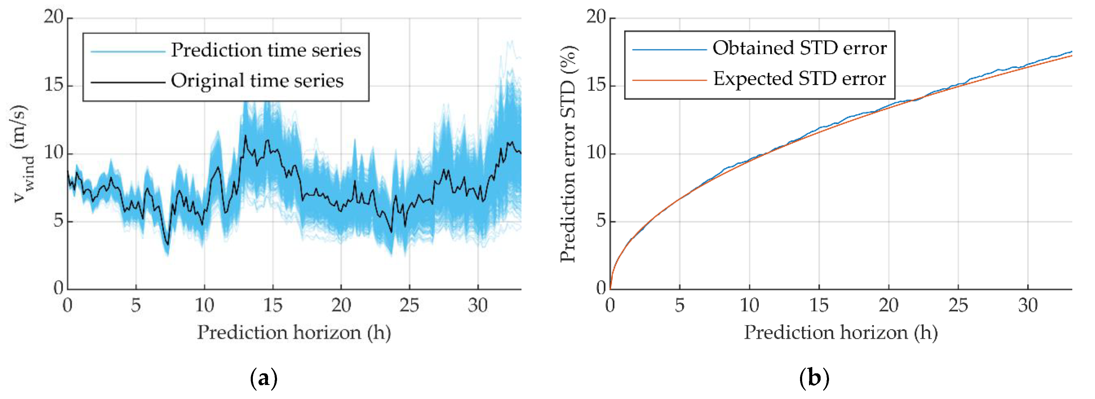
As an example of the results obtained with this method, Figure 2a shows an original wind speed time series and the prediction series created. Note that the prediction error tends to be higher as prediction horizon increases. Figure 2b shows that the desired STD error is reached.

3.2.2. Production Predictions Generation

Once the weather predictions are generated, it is possible to calculate the theoretical power produced by the wind turbines and solar photovoltaic (PV) panels. Then, after calculating the instant production in time, the total hourly production is calculated.

As for the wind production, the power is calculated using the $P-v$ curve corresponding to the wind turbines of the case study. Real wind speed ($v)$ values are taken from a weather station near the simulated HRES location. Then, the values are extrapolated to the wind turbine hub height, using Equation (5):

$$\frac{v\left(z\right)}{v\left(z_r\right)}={\left(\frac{z}{z_r}\right)}^{\alpha }$$

(5)

where $v\left(z\right)$ is the wind speed at hub height $z$, $v\left(z_r\right)$ is the wind speed at the weather station anemometer height $z_r$, and $\alpha$ is the power law exponent, which is calculated by using the expression proposed by Counihan [24] in Equation (6):

$$\alpha =0.096 {\log }_{10}{z}_0+0.016 {\left({\log }_{10}{z}_0\right)}^2+0.24$$

(6)

where $z_0$ is the surface roughness, which for this case is taken as $0.1 m$, referring to an area with few trees.

Regarding the solar power production, it is assumed that the PV panels produce the maximum power available for each of the weather conditions. The power is calculated with Equation (7):

$$P_{solar}=P_{STC}\left(1+\gamma \left(T_{cell}-25\right)\right)\frac{G}{1000}$$

(7)

where $P_{STC}$ refers to the maximum solar power at standard test conditions (STC),$P_{solar}$ is the solar power produced at $T_{cell}$ $(°\mathrm{C})$ cell temperature and $G$ irradiance $\left(W/m^2\right)$ conditions, and $\gamma$ $\left(°{\mathrm{C}}^{-1}\right)$ is the power coefficient of the module. The cell temperature is calculated with Equation (8).

$$T_{cell}=T_{air}+\left(NOCT-20\right)\frac{G}{800}$$

(8)

where $T_{air}$ is the ambient air temperature and $NOCT$ refers to the cell temperature at nominal operating conditions $\left(G=800\mathrm{W}/{\mathrm{m}}^2, T_{amb}=20 °\mathrm{C}, v_{wind}=1 \mathrm{m}/\mathrm{s}\right)$. This value is usually included in the solar module datasheet.

4. Battery Modelling

Both the energy efficiency of the battery and its state of health (SOH) are considered in the battery model.

The energy efficiency is modelled in terms of the power given by the battery, in contrast to other similar studies in which it is modelled as constant. An equivalent circuit model (ECM) is used to obtain the static response. The model consists of an ideal voltage source $\left(OCV\right)$ and a series resistance $\left(R_s\right)$. By using this model, the corresponding energy efficiency curves are obtained. Equations (9) and (10) define the efficiency for charging and discharging cases, respectively:

$${\eta }_{chg}\left(P_{int}\right)=\frac{P_{int}}{P_{ext}}=\frac{OC{V}^2}{OC{V}^2+R_s P_{int}}$$

(9)

$${\eta }_{dis}\left(P_{int}\right)=\frac{P_{ext}}{P_{int}}=\frac{OC{V}^2-R_s P_{int}}{OC{V}^2}$$

(10)

The battery efficiency is defined as the relationship between internal and external measured power and varies depending on the flow direction. The efficiency is expressed in terms of the internal power since the optimization uses this variable.

Regarding the SOH of the battery, this parameter can be defined as the current maximum capacity of the battery compared to its nominal value. In this study, the SOH is calculated using the Wöhler method [25,26]. This method is an event-oriented ageing model which calculates the battery degradation based on the performed charging and discharging cycles. The Wöhler method has been previously used in similar studies [11,27,28], and it is suitable due to its simplicity and sufficient accuracy for long-term simulation, like the ones to be conducted.

The method calculates the resting lifetime of the battery based on the relationship between the number of cycles already performed and the maximum number of cycles for its end of life. The maximum number of cycles varies depending on the depth of discharge (DOD), and on the type of battery. For this study, the data are taken from [29]. The total loss of life $\left(LL\right)$ is calculated with Equations (11) and (12):

$$LL={\displaystyle \sum }_{i=1}^{n_{ranges}}L{L}_i$$

(11)

$$L{L}_i=\frac{n_{cycles}^i}{N_{cycles}^i}$$

(12)

where $L{L}_i$ is the loss of life given in each DOD range, $n_{cycles}^i$ is the number of cycles given at that range, and $N_{cycles}^i$ is the maximum number of cycles for its end of life at that range. From Equation (11), it is possible to calculate the remaining lifetime as follows:

$$Lifetime \left(years\right)=\frac{1}{L{L}_{year}}$$

(13)

where $L{L}_{year}$ is the loss of life given in a year.

The number of cycles performed in a certain period of time is calculated using the Rainflow cycle counting algorithm [30].

5. Optimization Problem

In order to perform the sensitivity analysis, different forecast error curves are going to be tested for the same optimization strategy. The optimization is conducted using a particle swarm optimization (PSO) algorithm, which enables solving the nonlinear terms of the cost function. The optimization algorithm has two performance terms: enhancing the final profitability and minimizing the battery loss of value.

5.1. Optimization Algorithm

Particle swarm optimization is a heuristic optimization methodology, first presented by Kennedy and Eberhart [31], used to solve nonlinear functions. The main basis is to find a solution to the problem by iteratively modifying some initial possible solutions, named particles. The formulation used in this article introduces an inertia weight term, which was firstly presented by Shi and Eberhart [32], and which defines the balance between exploration and exploitation around the possible solutions domain.

$$v_i\left(k+1\right)=w_i\left(k\right) v_i\left(k\right)+{\phi }_1\left(x_{i,best}-x_i\left(k\right)\right)+{\phi }_2\left(x_{best}-x_i\left(k\right)\right)$$

(14)

$$x_i\left(k+1\right)=x_i\left(k\right)+dt v_i\left(k\right)$$

(15)

Equation (14) defines the speed $\left(v_i\right)$ by which particles change their position $\left(x_i\right)$, which is calculated in Equation (15). The meanings of each variable and parameter are summarized in

Table 2. Variables used in particle swarm optimization algorithm.

Variable	Definition
$v_i$	Speed of particle $i$
$x_{i,best}$	Best local position for particle $i$
$x_i$	$i$th particle position
$x_{best}$	Best global position

and

Table 3. Parameters used in particle swarm optimization algorithm.

Parameter	Definition	Value
$w_i$	Inertia weight for particle $i$	[0.4, 1]
${\phi }_1$	Exploration random uniform value	[0.5, 1]
${\phi }_2$	Exploitation random uniform value [${\phi }_{2 min}$, ${\phi }_{2 max}$]	[0.5, 1]
$dt$	Position update term	1
Nº of particles	Number of particles used in each optimization	200
$ite{r}_{max}$	Maximum number of iterations in each optimization	2000

.

The inertia can be calculated in many different ways, and after different comparisons, the linear time-varying method has been found to give better results for this particular case [33]. Equation (16) shows the corresponding formulation:

$$w_i\left(k\right)=\frac{ite{r}_{max}-n_{iter}}{ite{r}_{max}} \left(w_{i max}-w_{i min}\right)+w_{i min}$$

(16)

where $n_{iter}$ is the number of the current iteration, and $w_{i min}$ and $w_{i max}$ are the minimum and maximum inertia values, respectively, defined in Table 3.

One of the main benefits of selecting this optimization technique is the few number of parameters needed to adjust in order to solve a problem. Besides, its suitability for solving energy-related optimization problems has been proven in previous studies [34,35,36,37].

5.2. Cost Function

The optimization problem covers two aims: maximizing the profits obtained by the plant and minimizing the loss of value.

From the optimization point of view, the profits obtained from wind and solar energy production are constant since they rely on the predictions. Thus, the only variable term considered for the optimization is the profit obtained with the battery at each hour. The battery profits are calculated based on the energy given (positive) or received (negative) by the battery $\left(E_{give ba{t}_h}\right)$ and the electricity price predictions $\left(pric{e}_h\right)$ for each bidding period, which in the Iberian Electricity Market corresponds to an hour.

As explained in the battery modelling section, the energy losses vary depending on the power given/received by the battery. Thus, the given energy can be expressed in terms of the internal energy of the battery at the end of each hour $\left(E_{ba{t}_h}\right)$, considering that the energy is supplied at constant power. Equations (17) and (18) define the energy given for charging and discharging cases:

Charge:

$$E_{give ba{t}_h}=\frac{1}{{\eta }_{ch{g}_h}}\left(E_{ba{t}_{h-1}}-E_{ba{t}_h}\right)$$

(17)

Discharge:

$$E_{give ba{t}_h}={\eta }_{di{s}_h}\left(E_{ba{t}_{h-1}}-E_{ba{t}_h}\right)$$

(18)

where ${\eta }_{ch{g}_h}$ and ${\eta }_{di{s}_h}$ are the energy efficiencies at hour $h$ for charging and discharging cases, respectively, calculated with Equations (9) and (10).

With these considerations, the variables to be optimized at each case are the energy left in the battery at the end of each hour.

Regarding the loss of value of battery, this term aims to embrace both battery usage and technology degradation. The usage degradation, as explained in the battery modelling section, is calculated by its loss of life $\left(LL\right)$ related to the cycles performed, using the Wöhler method. The technology degradation is covered by considering the expected price decrease [7,38].

Using the price values and estimations reported by Bloomberg New Energy Finance [38], an exponential trend line has been modelled, as shown in Equation (16), defining the battery unit price $\left(UP\right)$ in (€/kWh).

$$U{P}_{day}=162.3 e^{-0.1029 \frac{d}{365}}$$

(19)

where $d$ corresponds to the day being analyzed, starting from 1 January 2018.

Thus, considering both the $LL$ and technology devaluation, the loss of value $\left(L{V}_{bat}\right)$ of the battery for a determined time span is defined in economic terms as follows:

$$L{V}_{bat}=E_{nom} U{P}_{day} \left(1-L{L}_{after opt}\right)-E_{nom} U{P}_{day-1} \left(1-L{L}_{prev}\right)$$

(20)

Therefore, considering both profit maximization and loss of value minimization, the cost function for the optimization problem is defined as:

$$max {\displaystyle \sum }_{h=1}^{N_h}{E}_{give ba{t}_h} pric{e}_h-L{V}_{bat}$$

(21)

where $N_h$ is the number of optimized hours, which varies depending on the market (see Table 1).

5.3. Bounds and Constraints

The bounds for the optimization variables, which are the energy of the battery at the end of each hour, are related to its minimum and maximum state of charge (SOC). For this case, minimum and maximum values of 20% and 80% have been considered, respectively. Avoiding complete charging or discharging of the battery aims to enhance the battery lifetime, as explained in [39].

Regarding the constraints, the given energy at each hour is limited first by the maximum power. This is modelled by Equations (22) and (23).

$$E_{ba{t}_h}-E_{ba{t}_{h-1}}\le P_{max bat chg} h$$

(22)

$$E_{ba{t}_{h-1}}-E_{ba{t}_h}\le P_{max bat dis} h$$

(23)

where $P_{max bat chg}$ and $P_{max bat dis}$ are the maximum power for charging and discharging cases and are limited by their respective efficiencies.

Secondly, in the studied case it is not allowed to charge the battery from the grid. Thus, the maximum charge of the battery for each hour is limited by the corresponding energy and solar production $\left(E_{ge{n}_h}\right)$.

$$E_{ba{t}_{h-1}}-E_{ba{t}_h}\le E_{ge{n}_h} {\eta }_{chg}\left(E_{ge{n}_h}\right)$$

(24)

Finally, the last constraints are linked to the energy SOC of the battery at the end of the day. To avoid reaching a minimum SOC value, which would limit the strategy for the following optimization day, a SOC interval is defined for the end of the day.

$$E_{bat 24}\ge \frac{SO{C}_{24 min}}{100}{E}_{nom}$$

(25)

$$E_{bat 24}\le \frac{SO{C}_{24 max}}{100}{E}_{nom}$$

(26)

where $SO{C}_{24 min}$ and $SO{C}_{24 max}$ are the minimum and maximum SOC values at the end of the day, respectively. In this case, they are set to 55% and 65%, respectively.

5.4. Algorithm Initialization Methods

Since heuristic algorithms such as PSO do not always assure finding the global optimal solution, different initialization methods are used to make sure that a profitable result is always obtained.

5.4.1. Random Initialization

In this first method, the initial particles are created in a completely random way.

5.4.2. LP Result-Based Initialization

For this second method, a linear programming (LP) optimization [40] is performed first for a simplified cost function of the case. In order to be linear, this function does not consider neither the battery degradation, nor the energy efficiency:

$$\mathit{max}{\displaystyle \sum }_{h=1}^{24}\left(E_{ba{t}_{h-1}}-E_{ba{t}_h}\right) pric{e}_h$$

(27)

Once this LP solution is obtained, it is included inside the initial population. The rest of the initial particles are created based on this LP result by applying random multiplying factors to it. This way, the LP result improvement is assured.

5.4.3. No Battery Use Initialization

This third method is used when the profit obtained with the previous two methods is below the one achievable without using the battery in that optimization period. In this case, the initial particles are created based on a result in which the battery is not used. Applying this strategy, for the given predictions, a nonnegative result is always ensured.

Besides, it should be noted that, in intraday market optimizations, for the three methods, previous optimization results are considered into the new initializations to accelerate the solution convergence and improve the previously found solution.

6. Case Study

6.1. Hybrid Plant

The hybrid renewable plant characteristics are defined in

Table 4. Case study hybrid plant data.

Parameter	Value
Solar power	30 MW
Wind power	50 MW
$P_{ext max bat}$	10 MW
$E_{nom bat}$	50 MWh
${\eta }_{chg}\left(P_{ext max bat}\right)$	96.07%
${\eta }_{dis}\left(P_{ext max bat}\right)$	95.54%

. Solar panels are modelled using the datasheet for Atersa ULTRA A-255 modules [41]. The wind turbines selected are the WindPACT 1.5 MW reference wind turbines from the NREL [42]. As for the battery, the efficiency modelling is based on the datasheet of LifeBatt X-2E 15Ah 40166 Li-ion cells.

The plant is considered to be located in the province of Araba, in Spain, and data for year 2018 have been taken for the study. The weather data are taken from the Basque Meteorological Agency, Euskalmet [43].

6.2. Sensitivity Analysis

A quantitative sensitivity analysis is performed by simulating the plant operation for a complete year with different setups. The first aim is to analyze the effects of applying different forecast errors. The second objective is to perform a comparison between the results obtained bidding only in the day-ahead market or bidding both in day-ahead and intraday markets.

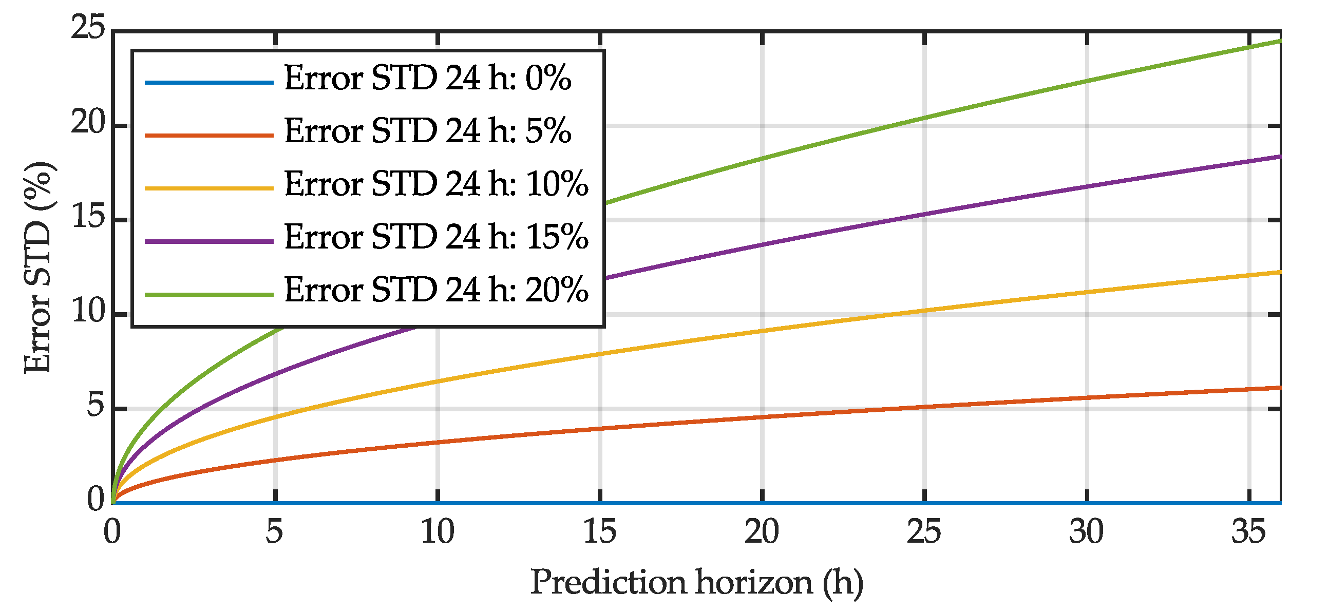
As for the forecast error cases, different levels of errors are modelled applying the square root error STD functions. The error STD values at 24 h prediction horizon are: 0% (no error case), 5%, 10%, 15%, and 20%. The error standard deviation curves are shown in Figure 3.

7. Results and Discussion

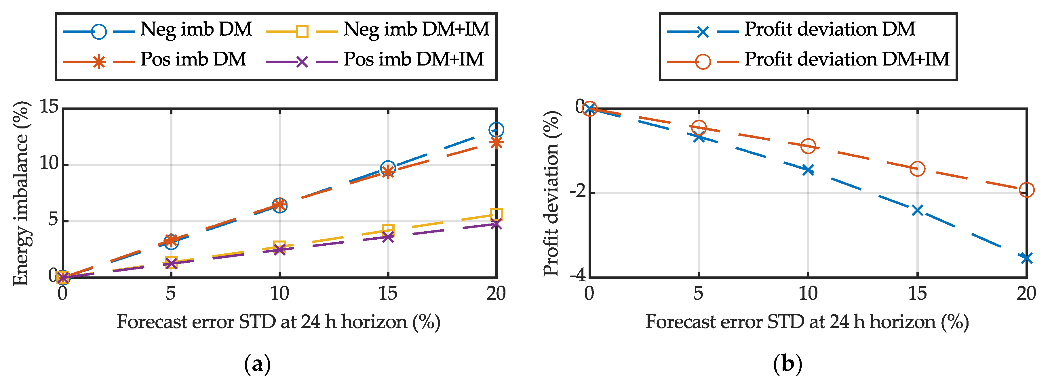
Simulations have been conducted using an Intel Core i7 CPU with 16 GB of RAM. With the selected parameters, each optimization is performed in less than 40 s. Figure 4 shows the energy imbalances and profit deviations obtained from the forecast error cases both for day-ahead (DM) and combined day-ahead and intraday market (DM + IM) participation.

In Figure 4a, the mean positive and negative deviations between the committed energy production and the real production are shown. It should be noted that, during real-time simulation, no control actions are taken to compensate these deviations since the aim is to analyze the effects of the forecasting errors. As for the imbalances, the result is consistent since the energy imbalance increases as the forecast uncertainty rises. Besides, similar results are obtained for positive and negative imbalances, which matches with the applied Brownian movement normal distribution.

Figure 4b shows the difference between the total received profit after applying imbalance penalties and the original schedule profit. As happens with the energy imbalances, the result is consistent since higher deviations are obtained for cases in which the forecast error STD is higher. Nevertheless, the profit deviation is not as high as the energy imbalance. This result is given for two reasons. First, the difference is conditioned by the imbalance penalties. Based on real data, these are taken as 13% for positive imbalances and 14% for negative imbalances. Second, it must be considered that the penalty is applied to the hourly price, influencing the final result.

Finally, in both energy and price deviation results, it is observed that, participating in intraday markets, both energy imbalances and profit deviations are significantly reduced.

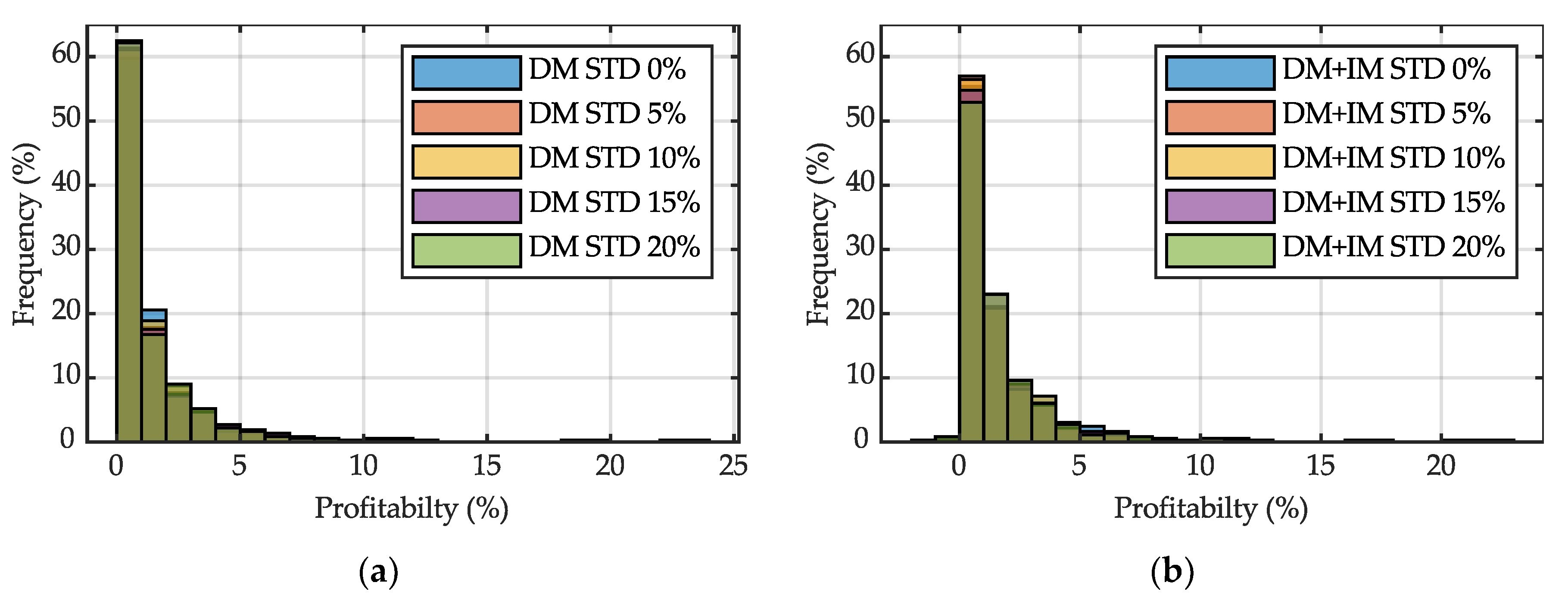
Figure 5 shows the battery profitability frequency distributions for day-ahead market participation strategy and for the combined day-ahead and intraday market participation strategy. In both cases, the profitability obtained with the battery is not high, showing slightly better results when intraday market participation is included. This is related to the fact that, in intraday markets, forecast errors are usually lower and, thus, more precise bidding decisions are taken.

Table 5. Results obtained for day-ahead market participation simulations.

Case	Relative Plant Profits (%)	Mean Battery Profitability (%)	Lifetime (Years)
0% STD	100	1.37	28.55
5% STD	99.11	1.35	28.99
10% STD	98.25	1.36	28.62
15% STD	97.39	1.31	30.13
20% STD	96.61	1.32	29.73

,

Table 6. Results obtained for day-ahead and intraday market participation simulations.

Case	Relative Plant Profits (%)	Mean Battery Profitability (%)	Lifetime (Years)
0% STD	100	1.50	41.11
5% STD	99.61	1.44	45.60
10% STD	99.25	1.45	44.14
15% STD	98.91	1.48	44.83
20% STD	98.58	1.49	43.50

and

Table 7. Comparison between the total profits obtained with day-ahead market (DM) participation and both day-ahead and intraday market (DM + IM) participations for different forecast uncertainties.

Case	Relative Plant Profits (%)
	DM	DM + IM
0% STD	99.91	100
5% STD	99.02	99.61
10% STD	98.16	99.25
15% STD	97.30	98.91
20% STD	96.52	98.58

show the numerical results obtained for each performed complete year simulation. Table 5 shows the results obtained for just day-ahead market participation, Table 6 shows the results for day-ahead and intraday markets participation, and Table 7 provides a comparison between the profits obtained in each case, in relative terms.

The plant profits decrease in simulations in which the forecast uncertainty increases. Nevertheless, as can be observed in Figure 4b, the profit variation is lower when intraday market participation is applied. In addition, in contrast to the plant profit results, the battery profitability remains almost unchanged for different forecast error cases. The same effect is observed in the remaining battery lifetime at the end of the year. The reason for this is that the main parameter which affects the battery profitability and usage is the price difference and, as this parameter does not change between different simulations, neither does the battery usage strategy.

The small variations between simulations are caused by the effect of the production forecasts in the optimization, since the strategy establishes that the batteries cannot be charged from the grid. As a result, the mean profitability is slightly higher when intraday market participation is performed. The same happens with the battery lifetime.

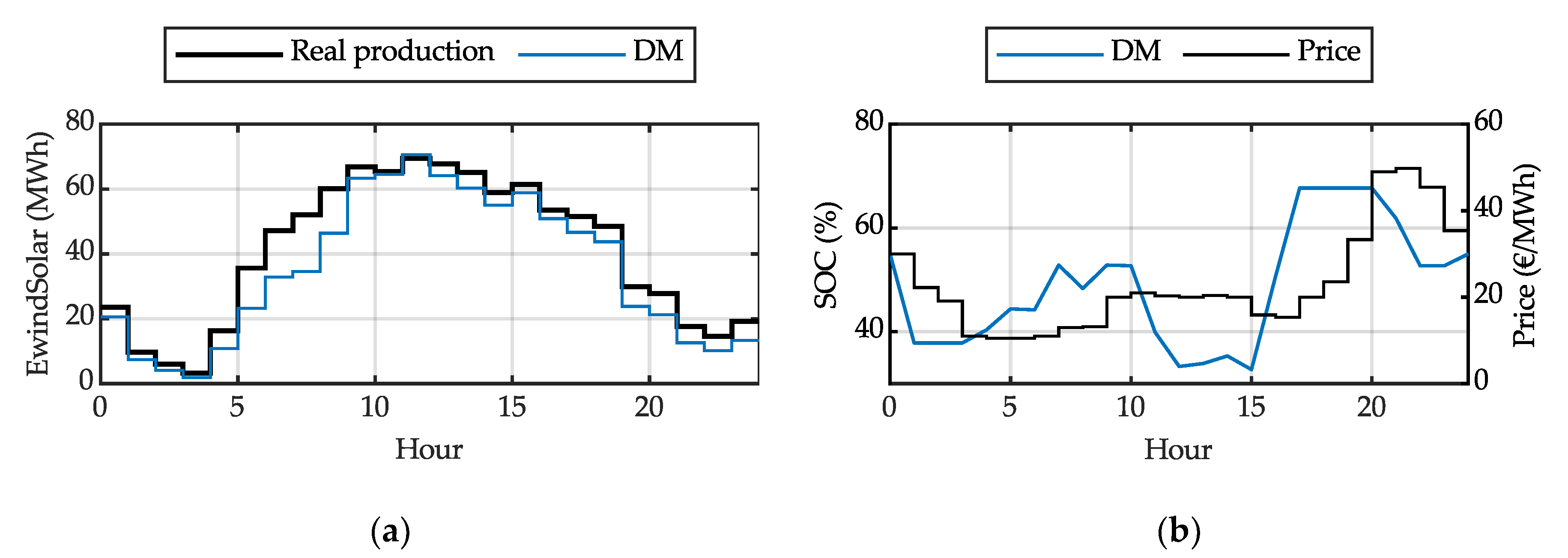
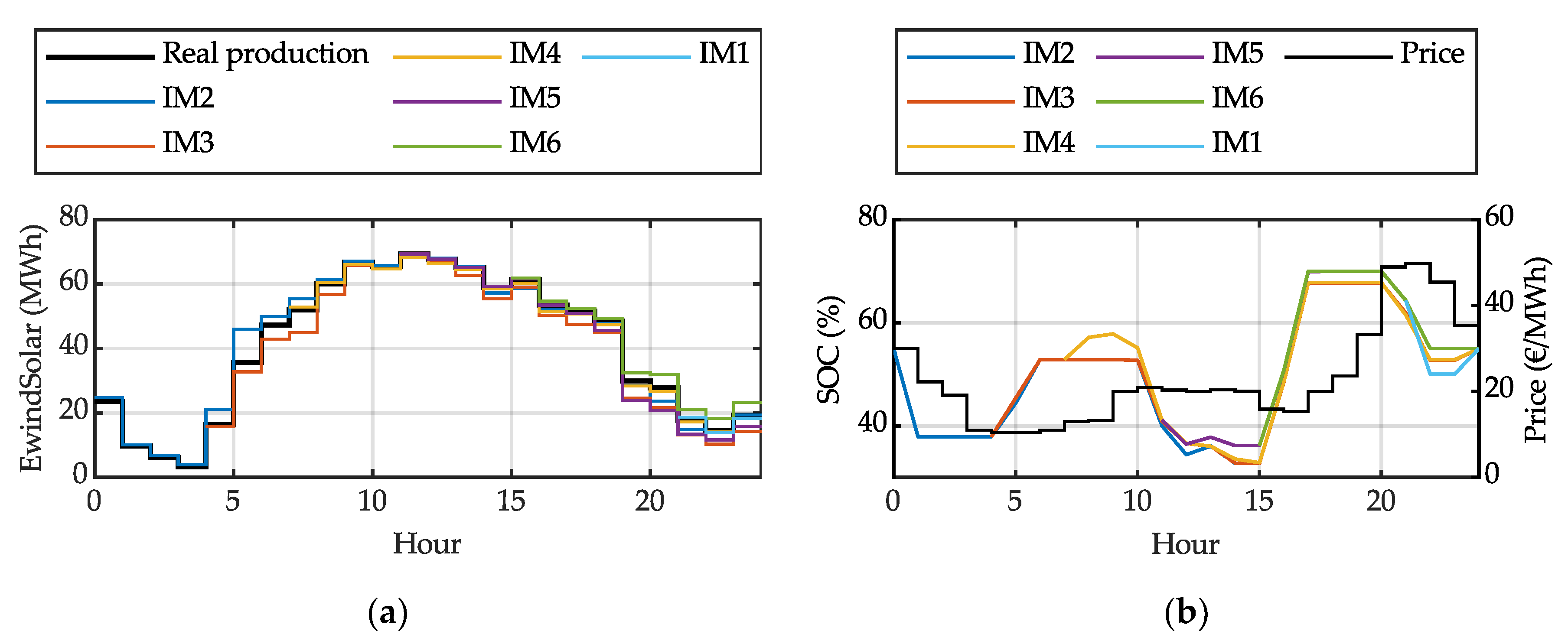
The effects of participating in intraday markets are better analyzed in a particular day case. As an example, the results obtained for day 83 (24/03/2018), with a forecast error STD of 10% at 24-h prediction horizon, are analyzed.

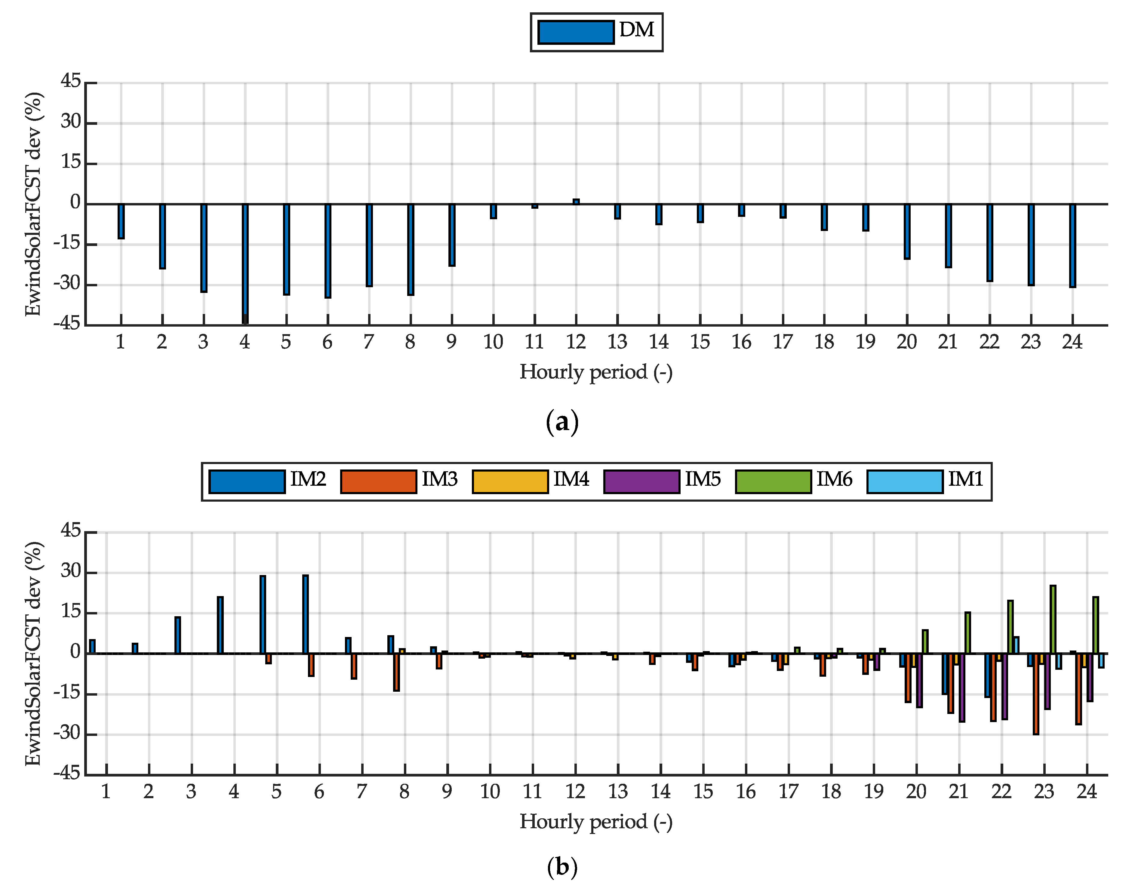
Figure 6a and Figure 7a show the real plant production curve (wind and solar production) versus the predictions conducted at market auction time. Even if, due to the normal distribution, results can vary, by participating in intraday markets, usually more accurate weather predictions are done and, thus, better production predictions. This effect is noted in Figure 8, where the deviation between real production and production estimations is shown.

Figure 6b and Figure 7b show the different SOC curve strategies obtained from the optimization, as well as the applied price predictions (which, as explained before, are kept constant for different optimizations). The SOC strategy varies slightly for different market bids. The reason for this could be that the new prediction causes a new optimization result or that PSO does not always find the global best solution. Nevertheless, for new optimizations during intraday markets, the previous optimization result is considered. Thus, the new result improves or keeps the previous solution. Furthermore, the results have a great similarity.

Finally,

Table 8. Comparison between the results obtained for only day-ahead (DM) and both day-ahead and intraday market (DM + IM) participation for day 83 with 10% forecast error STD at 24-h prediction horizon.

Parameter	DM Strategy	DM + IM Strategy
Total profit	20,183.89 €	20,518.06 €
Battery profit	408.44 €	475.47 €
Battery net profitability	2.07%	2.37%
Positive energy imbalance	13.56%	1.14%
Negative energy imbalance	−0.12%	−1.64%
Loss of life of the day	6.52e-3%	9.21e-3%

summarizes the results obtained for each market participation strategy. From the table, it is concluded that energy imbalances are reduced considerably, which involves obtaining higher total profits. Besides, for this particular day case, with the intraday market participation the battery usage is more efficient. Thus, a higher profitability is obtained.

8. Conclusions

A sensitivity analysis has been conducted for a HRES with a battery energy storage system. First, the effects of forecast errors have been analyzed. Second, the benefits of participating in intraday markets have also been assessed. All the simulations have been conducted for a complete year using real data in order to obtain realistic results.

Regarding the sensitivity analysis, the results show that even if energy deviations increase considerably as forecast uncertainty rises, the total profits obtained by the plant do not change substantially. As for energy arbitrage, the profitability obtained is not high and this is caused by the small price deviations in the Iberian Electricity Market. Performing energy arbitrage is important to obtain as much profitability as possible from the price differences in the market, but if these price differences during the day are not high, neither are the benefits obtained from performing this strategy. For that reason, there are cases during the year in which the usage of the battery for arbitrage is not compensated with the cost related to the cycling degradation. In these cases, the optimization algorithm establishes that the battery is not going to be used. This is the reason why such a long life estimation has been obtained at the end of the year in all simulations. Besides, no clear correlation is observed between the used forecast error STD curve and the profitability of the battery, since all the results are similar. This is consistent, as even if energy production constrains the battery strategy, the most limiting factor is usually the price difference, which does not change between simulations.

As for the market participation strategies, it has been proven that the participation in intraday markets enhances the profits and reduces the energy imbalances compared to only day-ahead market participation. This effect is higher as the forecast uncertainty rises.

A final point to note is that, even if profitability increases with intraday market participation, the benefits from performing energy arbitrage are not substantial in the Iberian Electricity Market. Thus, investing in a battery energy storage system just for energy arbitrage application may not be cost-effective. For this reason, as well as for arbitrage purposes, the battery system should be also considered for other remunerated applications such as providing ancillary services or compensating production curtailments. This subject will be treated in future studies.

References

- IRENA. Climate Change and Renewable Energy: National Policies and the Role of Communities, Cities and Regions; Report to the G20 Climate Sustainability Working Group (CSWG); International Renewable Energy Agency: Abu Dhabi, UAE, 2019. [Google Scholar]
- REE. Preview of the Report on The Spanish Electricity System 2019; Red Eléctrica de España: Madrid, Spain, 2020. (In Spanish) [Google Scholar]
- Denholm, P.; Ela, E.; Kirby, B.; Milligan, M. The Role of Energy Storage with Renewable Electricity Generation; National Renewable Energy Laboratory: Golden, CO, USA, 2010.
- Gomez, T.; Herrero, I.; Rodilla, P.; Escobar, R.; Lanza, S.; De La Fuente, I.; Llorens, M.L.; Junco, P. European Union Electricity Markets: Current Practice and Future View. IEEE Power Energy Mag. 2019, 17, 20–31. [Google Scholar] [CrossRef]
- Nehrir, M.H.; Wang, C.; Strunz, K.; Aki, H.; Ramakumar, R.; Bing, J.; Miao, Z.; Salameh, Z. A Review of Hybrid Renewable/Alternative Energy Systems for Electric Power Generation: Configurations, Control, and Applications. IEEE Trans. Sustain. Energy 2011, 2, 392–403. [Google Scholar] [CrossRef]
- Khare, V.; Nema, S.; Baredar, P. Solar–wind hybrid renewable energy system: A review. Renew. Sustain. Energy Rev. 2016, 58, 23–33. [Google Scholar] [CrossRef]
- Sánchez Muñoz, A.; Garcia, M.; Gerlich, M. Overview of Storage Technologies; Sensible Project: European Union’s Horizon 2020 Program; Project Sensible: Brussels, Belgium, 2016. [Google Scholar]
- Leadbetter, J.; Swan, L.G. Selection of battery technology to support grid-integrated renewable electricity. J. Power Sources 2012, 216, 376–386. [Google Scholar] [CrossRef]
- Korpaas, M.; Holen, A.T.; Hildrum, R. Operation and sizing of energy storage for wind power plants in a market system. Int. J. Electr. Power Energy Syst. 2003, 25, 599–606. [Google Scholar] [CrossRef]
- Saez-de-Ibarra, A.; Milo, A.; Gaztanaga, H.; Debusschere, V.; Bacha, S. Co-Optimization of Storage System Sizing and Control Strategy for Intelligent Photovoltaic Power Plants Market Integration. IEEE Trans. Sustain. Energy 2016, 7, 1749–1761. [Google Scholar] [CrossRef]
- Gonzalez-Garrido, A.; Saez-de-Ibarra, A.; Gaztanaga, H.; Milo, A.; Eguia, P. Annual Optimized Bidding and Operation Strategy in Energy and Secondary Reserve Markets for Solar Plants with Storage Systems. IEEE Trans. Power Syst. 2019, 34, 5115–5124. [Google Scholar] [CrossRef]
- Wang, J.; Zhong, H.; Tang, W.; Rajagopal, R.; Xia, Q.; Kang, C.; Wang, Y. Optimal bidding strategy for microgrids in joint energy and ancillary service markets considering flexible ramping products. Appl. Energy 2017, 205, 294–303. [Google Scholar] [CrossRef]
- Chen, Y.; Deng, C.; Yao, W.; Liang, N.; Xia, P.; Cao, P.; Dong, Y.; Zhang, Y.; Liu, Z.; Li, D.; et al. Impacts of stochastic forecast errors of renewable energy generation and load demands on microgrid operation. Renew. Energy 2019, 133, 442–461. [Google Scholar] [CrossRef]
- Chen, Y.; Deng, C.; Li, D.; Chen, M. Quantifying cumulative effects of stochastic forecast errors of renewable energy generation on energy storage SOC and application of Hybrid-MPC approach to microgrid. Int. J. Electr. Power Energy Syst. 2020, 117, 105710. [Google Scholar] [CrossRef]
- Fabbri, A.; Gómez San Román, T.; Rivier Abbad, J.; Méndez Quezada, V.H. Assessment of the Cost Associated With Wind Generation Prediction Errors in a Liberalized Electricity Market. IEEE Trans. Power Syst. 2005, 20, 1440–1446. [Google Scholar] [CrossRef]
- Ding, H.; Pinson, P.; Hu, Z.; Song, Y. Optimal Offering and Operating Strategies for Wind-Storage Systems With Linear Decision Rules. IEEE Trans. Power Syst. 2016, 31, 4755–4764. [Google Scholar] [CrossRef]
- Head of the State. Law 54/1997, of November 27, on the Electricity Sector; Boletín Oficial del Estado: Madrid, Spain, 1997; pp. 35097–35126. (In Spanish)
- Ministry of Industry and Energy. Organisation and Regulation of the Electricity Production Market; Boletín Oficial del Estado: Madrid, Spain, 1997; pp. 1–20. (In Spanish)
- Ministry of Energy Tourism and Digital Agenda. Day-Ahead and Intraday Electricity Market Operating Rules; Boletín Oficial del Estado: Madrid, Spain, 2018; pp. 49415–49563. (In Spanish)
- Ministry of Industry, Energy and Tourism. Criteria for Participating in Ancillary Services; Boletín Oficial del Estado: Madrid, Spain, 2015; pp. 119723–119944. (In Spanish)
- ESIOS: System Operator Information System. Available online: https://www.esios.ree.es/es (accessed on 17 March 2020).
- Ayón, X.; Moreno, M.; Usaola, J. Aggregators’ Optimal Bidding Strategy in Sequential Day-Ahead and Intraday Electricity Spot Markets. Energies 2017, 10, 450. [Google Scholar] [CrossRef]
- Einstein, A. Investigations on the Theory of the Brownian Movement; Dover Publications: New York, NY, USA, 1956; ISBN 0-486-60304-0. [Google Scholar]
- Manwell, J.F.; McGowan, J.G.; Rogers, A.L. Wind Energy Explained: Theory, Design and Application; John Wiley & Sons: Hoboken, NJ, USA, 2009; ISBN 978-0-470-01500-1. [Google Scholar]
- Sauer, D.U.; Wenzl, H. Comparison of different approaches for lifetime prediction of electrochemical systems—Using lead-acid batteries as example. J. Power Sources 2008, 176, 534–546. [Google Scholar] [CrossRef]
- Badey, Q.; Cherouvrier, G.; Reynier, Y.; Duffault, J.-M.; Franger, S. Ageing forecast of lithium-ion batteries for electric and hybrid vehicles. Curr. Top. Electrochem. 2011, 16, 1–16. [Google Scholar]
- Sarasketa Zabala, E. A Novel Approach for Lithium-Ion Battery Selection and Lifetime Prediction. Ph.D. Thesis, Mondragon Unibertsitatea, Arrasate, Spain, 2014. [Google Scholar]
- Saez-de-Ibarra, A.; Herrera, V.I.; Milo, A.; Gaztanaga, H.; Etxeberria-Otadui, I.; Bacha, S.; Padros, A. Management Strategy for Market Participation of Photovoltaic Power Plants Including Storage Systems. IEEE Trans. Ind. Appl. 2016, 52, 4292–4303. [Google Scholar] [CrossRef]
- Herrera, V.I.; Saez-de-Ibarra, A.; Milo, A.; Gaztanaga, H.; Camblong, H. Optimal energy management of a hybrid electric bus with a battery-supercapacitor storage system using genetic algorithm. In Proceedings of the 2015 International Conference on Electrical Systems for Aircraft, Railway, Ship Propulsion and Road Vehicles (ESARS), Aachen, Germany, 3–5 March 2015; pp. 1–6. [Google Scholar]
- Downing, S.; Socie, D. Simple rainflow counting algorithms. Int. J. Fatigue 1982, 4, 31–40. [Google Scholar] [CrossRef]
- Kennedy, J.; Eberhart, R. Particle swarm optimization. In Proceedings of the ICNN’95—International Conference on Neural Networks, Perth, Australia, 27 November–1 December 1995; Volume 4, pp. 1942–1948. [Google Scholar]
- Shi, Y.; Eberhart, R. A modified particle swarm optimizer. In Proceedings of the 1998 IEEE International Conference on Evolutionary Computation Proceedings, IEEE World Congress on Computational Intelligence (Cat. No.98TH8360), Anchorage, AK, USA, 4–9 May 1998; pp. 69–73. [Google Scholar]
- Nickabadi, A.; Ebadzadeh, M.M.; Safabakhsh, R. A novel particle swarm optimization algorithm with adaptive inertia weight. Appl. Soft Comput. 2011, 11, 3658–3670. [Google Scholar] [CrossRef]
- Duchaud, J.-L.; Notton, G.; Darras, C.; Voyant, C. Multi-Objective Particle Swarm optimal sizing of a renewable hybrid power plant with storage. Renew. Energy 2019, 131, 1156–1167. [Google Scholar] [CrossRef]
- Zulueta, E.; Kurt, E.; Uzun, Y.; Lopez-Guede, J.M. Power control optimization of a new contactless piezoelectric harvester. Int. J. Hydrogen Energy 2017, 42, 18134–18144. [Google Scholar] [CrossRef]
- Dai, Q.; Liu, J.; Wei, Q. Optimal Photovoltaic/Battery Energy Storage/Electric Vehicle Charging Station Design Based on Multi-Agent Particle Swarm Optimization Algorithm. Sustainability 2019, 11, 1973. [Google Scholar] [CrossRef]
- Kien, L.C.; Duong, T.L.; Phan, V.-D.; Nguyen, T.T. Maximizing Total Profit of Thermal Generation Units in Competitive Electric Market by Using a Proposed Particle Swarm Optimization. Sustainability 2020, 12, 1265. [Google Scholar] [CrossRef]
- Bloomberg NEF. New Energy Outlook 2019; Bloomberg New Energy Finance: New York, NY, USA, 2019. [Google Scholar]
- Xu, L.; Yang, F.; Hu, M.; Li, J.; Ouyang, M. Comparison of energy management strategies for a range extended electric city bus. In Proceedings of the 31st Chinese Control Conference, Hefei, China, 25–27 July 2012; pp. 6866–6871. [Google Scholar]
- Rahimiyan, M.; Baringo, L. Strategic Bidding for a Virtual Power Plant in the Day-Ahead and Real-Time Markets: A Price-Taker Robust Optimization Approach. IEEE Trans. Power Syst. 2016, 31, 2676–2687. [Google Scholar] [CrossRef]
- ULTRA Line-Photovoltaic Modules-Atersa. Available online: http://atersa.com/en/products-services/photovoltaic-modules/ultra-line/ (accessed on 20 March 2020).
- Dykes, K.L.; Rinker, J. WindPACT Reference Wind Turbines; National Renewable Energy Laboratory: Golden, CO, USA, 2018; pp. 1–31.
- Open Data Euskadi. Available online: https://opendata.euskadi.eus/catalogo-datos (accessed on 20 March 2020).
Figure 1.
Standard deviation of the production prediction obtained by SIPREÓLICO tool for a specific week in a province of Spain.
Figure 2.
Wind speed prediction time series generation for 1000 cases. (a) Prediction time series and the original time series; (b) Expected and obtained prediction error standard deviation (STD).
Figure 3.
Error standard deviation (STD) cases used for the sensitivity analysis.
Figure 4.
Effects of applying forecast errors from the energetic and economic point of view. (a) Mean negative and positive energy imbalances between the scheduled and produced energy; (b) Relative profit deviation between the total real and scheduled profits.
Figure 5.
Battery profitability frequency histograms. (a) Profitability histogram for day-ahead market (DM) participation case; (b) Profitability histogram for day-ahead and intraday market (DM + IM) participation case.
Figure 6.
Results obtained for day 83 with a forecast error STD of 10% at 24-h prediction horizon for a day-ahead market participation strategy. (a) Real wind and solar production versus prediction at market auction time; (b) State of charge (SOC) strategy obtained from the optimization and price prediction for that day.
Figure 7.
Results obtained for day 83 with a forecast error STD of 10% at 24-h prediction horizon for a day-ahead and intraday market participation strategy. (a) Real wind and solar production versus predictions at market auction times; (b) State of charge (SOC) strategies obtained from the different optimizations and price prediction for that day.
Figure 8.
Comparison of the deviations between the real and predicted productions for the two market participation strategies. (a) Deviations for only day-ahead market participation strategy; (b) Deviations for combined day-ahead and intraday market participation strategy.