Article

Employing Machine Learning for Detection of Invasive Species using Sentinel-2 and AVIRIS Data: The Case of Kudzu in the United States

by
Tobias Jensen
,
Frederik Seerup Hass
,
Mohammad Seam Akbar
,
Philip Holm Petersen
and
Jamal Jokar Arsanjani
*
Department of Planning, Geography and Surveying, Aalborg University Copenhagen, A.C Meyers Vænge 15, 2450 Copenhagen, Denmark
*
Author to whom correspondence should be addressed.
Sustainability 2020, 12(9), 3544; https://doi.org/10.3390/su12093544
Submission received: 30 March 2020 / Revised: 20 April 2020 / Accepted: 22 April 2020 / Published: 27 April 2020

Abstract

:
Invasive plants are causing massive economic and environmental troubles for our societies worldwide. The aim of this study is to employ a set of machine learning classifiers for detecting invasive plant species using remote sensing data. The target species is Kudzu vine, which mostly grows in the south-eastern states of the US and quickly outcompetes other plants, making it a relevant and threatening species to consider. Our study area is Atlanta, Georgia and the surrounding area. Five different algorithms: Boosted Logistic Regression (BLR), Naive Bayes (NB), Neural Network (NN), Random Forest (RF) and Support Vector Machine (SVM) were tested with the aim of testing their performance and identifying the most optimal one. Furthermore, the influence of temporal, spectral and spatial resolution in detecting Kudzu was also tested and reviewed. Our finding shows that random forest, neural network and support vector machine classifiers outperformed. While the achieved internal accuracies were about 97%, an external validation conducted over an expanded area of interest resulted in 79.5% accuracy. Furthermore, the study indicates that high accuracy classification can be achieved using multispectral Sentinel-2 imagery and can be improved while integrating with airborne visible/infrared imaging spectrometer (AVIRIS) hyperspectral data. Finally, this study indicates that dimensionality reduction methods such as principal component analysis (PCA) should be applied cautiously to the hyperspectral AVIRIS data to preserve its utility. The applied approach and the utilized set of methods can be of interest for detecting other kinds of invasive species as part of fulfilling UN sustainable development goals, particularly number 12: responsible consumption and production, 13: climate action, and 15: life on land.

1. Introduction

1.1. Invasive Species

An invasive species is defined by the Executive Order 13112 as “an alien species whose introduction does or is likely to cause economic or environmental harm or harm to human health” [1]. Environmental damage happens when there is a significant decrease in native species, an alteration to plant and animal communities or to ecological processes that native species and other desirable plants, animals and humans depend on for survival [2]. There is a substantial problem with invasive species in the U.S., which is causing a lot of harm both economically and environmentally [3]. Invasive species are estimated to cost $120B annually and affect more than 100 million acres spread out across the entire country [4].
Invasive species can have widespread impacts on societies ranging from reduced agricultural output and reducing populations of native species significantly due to invasive species having a competitive advantage in their new environment. This skewing of competition can be seen in its effects on other species; 42% of all species that are categorized as either threatened or endangered are in large part listed in this way due to competing invasive species [5]. Remote sensing technology and methods offer an opportunity to detect many different objects and entities on the ground and at sea, which includes different plant species. The methodology used to detect different types of plants is rooted in the target plant’s unique characteristics [6,7].

1.2. Kudzu Vine and Its Phenology

One of the most widespread invasive species in the U.S. is the Kudzu vine, which was nicknamed “The vine that ate the south”. Kudzu outcompetes almost everything in its path at a fast pace. The vine entered North America in the late 1800s, after the World’s Fair in Philadelphia, which marked the event that introduced Kudzu. The plant originates from East Asia in the regions of China and Japan. It quickly became popular in the Americas in various planning and environmental departments, as it could be used to fight against erosion on slopes and hillsides or as a cover for slopes along highway and railways. For this reason, millions of seeds were spread across the south. These plants were not kept under control, which is the main reason Kudzu has spread so massively and has become a huge issue for the American government and landowners [8]. In order to detect Kudzu remotely, the phenology of the vine will be investigated, allowing us to take advantage of its characteristics and to get a better impression of the behavior of the vine.
The main objective of this study is to enhance the automatic detection of invasive plant species, more specifically the Kudzu vine, using remote sensing data [9]. Our approach is based on setting a set of machine learning classification algorithms on multispectral remote sensing data. The main challenge in detecting Kudzu lies in distinguishing it from surrounding vegetation. The key lies in its phenology: (a) a possible way of doing this could be to take advantage of the fact that Kudzu does not lose its leaves until the first winter frost [10], making the plant stand out among other vegetation in late fall and early winter, (b) another method would be to make use of its unique characteristic; compared to other vegetation, Kudzu has high concentration of nitrogen [10].
There are some existing studies on the subject related to remote sensing and machine learning classification. Two recent studies are particularly relevant to this study, with the first being a study on the use and possibilities of different remote sensing data. The study [11] summarizes different approaches for detecting invasive alien species using general remote sensing techniques. The case the study focused on is the South American Solanum Mauritianum, more commonly referred to as Bugweed, which is becoming an increasing problem in South African forest areas. S. Mauritianum is not very easily distinguished from other vegetation, due to its neutral green color and ability to grow both at the canopy level and below. The study also states that remote sensing of invasive plant species has typically been focused on high spatial resolution aerial imagery, but also states that these products have their limitations. A key factor in success with such products involves considering the plant’s unique abilities such as its flowering and fruiting seasons. Performing time series analysis with high-resolution imagery has proven to be an effective detection method that is made possible by having sub-meter satellite imagery. However, relying only on imagery makes it very difficult to detect species that do not clearly distinguish themselves from their surroundings, and higher resolution does not solve this problem.
Even multispectral products can struggle in detecting plants that exhibit similar characteristics to their surroundings. Overall the results are better when using multispectral products over just optical ones but these products still struggle when vegetation cover is sparse. The field of detecting invasive plant species is therefore shifting towards hyperspectral data, which shows advantages over optical and multispectral products. Hyperspectral data has proven to be much more capable in distinguishing vegetation types from each other, due to the possibility of obtaining each species’ exact spectral signature [12]. Relying on hyperspectral data does though have its limitations. While hyperspectral data does yield better results (usually above 80% accuracy), it is mostly limited to aerial products, such as HyMap and airborne visible/infrared imaging spectrometer (AVIRIS) [13]. These aerial products have a major disadvantage in large scale mapping of being very costly, making the economic advantage of remote sensing less obvious. The required amount of accuracy needs to be considered, since very accurate mapping comes at a cost. Remote sensing products with a high temporal resolution, such as satellite imagery, might still have an advantage in cost and scaling, even though their results are less accurate [14].
The second relevant study is a study by D. McIntyre [15], which aims to use remotely sensed data to detect and map the invasive plant species “Paterson’s curse” in Western Australia. Paterson’s curse is detectable because of its ability to stay green for longer than other plants, thereby making it possible to identify among other types of vegetation. If the Paterson’s Curse is not detected in the late stages of its yearly vegetation lifespan, it is also detectable through its two weeks flowering period. This is mainly because of its blue flowers, which make it very detectable in a blue color index. Because the flowering season is crucial to the performance of the detection, it does not leave much room for data collection, which is both concerning for field work and for remote sensing data. When the detection is highly dependent on a short-lived flowering season, remote sensing detection can become very challenging. The points of flowering and late seasonal aging discussed in the concluding parts of this study are considered to be the most crucial ones in the detection of this invasive species. When evaluating the importance of data resolution, the study finds that spectral resolution is more important than spatial resolution. It also finds that high spatial resolution imagery is not much better than medium resolution imagery, due to lack of spectral bands. Hyperspectral satellite imagery with a 30-m resolution is ideal for detecting certain types of weeds. Such data used to be available from the Hyperion EO-1 satellite before it shut down in 2017. The EnMap satellite will provide this data from 2020, providing a bright future for the detection of weeds. At the moment, airborne hyperspectral imagery is just as suitable as satellite data, but of course at a much higher cost. Due to the high cost of airborne data, the study suggests using satellite remote sensing to locate areas with a potential for a large number of invasive species and to focus the airborne data collection at these areas. Airborne data does also leave more flexibility in exactly when the data collection is happening, and flowering periods can be used very efficiently in this way.
The study primarily uses two classifiers: Multilayer Perceptron and K-Nearest Neighbour. These two algorithms were used because past studies found these performing well in similar classifications [16]. The results reach an overall accuracy from both models around 66%. Overall the study is more focused on the methodology in detecting invasive species with remote sensing rather than on actually applying machine learning in the process. Knowing the specific plant characteristics and how it behaves in its surroundings is a crucial factor in detecting it [17]. The findings of the study further suggest that satellite imagery is capable of mapping weeds, but only to a certain degree of accuracy. Hyperspectral imaging has proven to be more suitable, whether it involves satellite or airborne collected data. A combination of the two is not covered. Since the study by D. McIntyre [15] revolves around the flowering period of the plant, long-term temporal resolution is not covered as a factor. That leaves the question of spectral resolution versus temporal resolution. With the findings of the two studies, further investigation on how machine learning and the use of combining multiple data sources can increase the possibilities in the detection of Kudzu. With the question of hyperspectral data versus long term temporal data still being open from the literature, this aspect will be examined further in this study.

1.3. Objectives and Research Questions

The primary objective of the study is to assess the suitability of a set of machine learning algorithms for detecting the Kudzu vine using remote sensing data. Furthermore, the study seeks to examine how changing different parameters and processing approaches affect accuracy results across the selected algorithms. Sentinel-2 is deemed suitable to detect Kudzu, using the yearly growth cycle of the plant to identify the plant among other objects. The end goal is to produce a binary land cover classification showing the extent of Kudzu growth in the study area. Based on our literature review, the following research questions arise:
  • How accurately can Kudzu be classified using different machine learning algorithms on Sentinel-2 multispectral images versus AVIRIS hyperspectral data?
  • What differences will be seen using several seasonal multispectral images compared to a single hyperspectral image?
  • How does combining multispectral and hyperspectral data affect overall accuracy and does resampling have any influence on the result?

2. Data and Method

2.1. Area of Interest

The study area was defined based on the availability of data. This resulted in an area which is a combination of one Sentinel image tile and part of one AVIRIS flight path. The final study area was the AVIRIS flight path located within the Sentinel tile and can be seen as the orange area marked in Figure 1.

2.2. Data

2.2.1. Remote Sensing Data

Sentinel-2

Based on its high temporal resolution together with good spatial and spectral resolution, Sentinel-2 was decided to be suitable for the study. During the phenology investigation of Kudzu, it was discovered that the vine exhibits traits in its yearly cycle which are distinct from other vegetation. As a result, using a multitemporal approach for the detection of the plant would make sense. Due to Sentinel’s relatively short revisit frequency, it was suitable for our research purposes. Furthermore, the Sentinel-2 program was recently launched and has capabilities that are suitable for vegetation monitoring [18]. From each season throughout 2017, one cloud-free composite image was used. The image capture periods are the following, shown in Table 1:
The Sentinel-2 composites were combined into a single layer stack. The stack consists of four Sentinel-2 images with the indices made from those images. The indices in question were extracted from Tasseled cap transformation i.e., brightness, greenness and wetness as well as the Soil-Adjusted Vegetation Index (SAVI). For each of the Sentinel-2 images, the band numbers 2, 3, 4, 5, 6, 7, 8, 8a, 11 and 12 were used. This resulted in a single stack of 56 image bands.

AVIRIS

The publicly available hyperspectral AVIRIS data can freely be downloaded from the AVIRIS data portal. AVIRIS collects data in 224 different spectral bands, each with a wavelength of 10 nm in a total wavelength span of 400 to 2500 nm, the spatial resolution is 16.6 m [19]. The AVIRIS data was captured on 18 April 2017, and all 224 bands were used in the machine learning model. Preprocessing was done in ArcMap [Version 10.6.1].
In order to stack data from Sentinel-2 and AVIRIS, the data products had to be resampled into equal pixel sizes. The Sentinel-2 bands 5, 6, 7, 8a, 11, and 12 needed to be resampled from 20 m to 10 m before stacking the Sentinel-2 images. For the analysis, which tested how resampling affects results, Sentinel-2 data was resampled to 16.6 m from 10/20 m and AVIRIS was resampled to 10 m from 16.6 m.

2.2.2. Ground Truth Data

The most comprehensive dataset for invasive species in the US is made by EDDMapS, a map and data service developed by The University of Georgia–Center for Invasive Species and Ecosystem Health. EDDMapS collects information on all known invasive species, both animals and plants, by combining existing datasets in addition to volunteers reporting their observations [20]. The dataset is not very consistent in its structure, mostly due to some of it being produced by volunteers. The desired coverage for a ground truth area is a minimum of 1000 m2, which is secured by a careful selection of records.
With the use of NAIP Orthophotos, Google Maps and Google Street View, the ground truth data points were verified and a cluster of points was created at each location. This resulted in a total of 366 points dispersed over 17 known locations of Kudzu. The second data set that needs to be sampled includes the points representing everything but Kudzu. It is important to make sure that these points fulfill this criterion, which is why every point was individually reviewed to make sure that the points do not represent Kudzu.
This ensured that the data set is accurate, which enabled the machine learning classifiers to distinguish Kudzu pixels from non-Kudzu pixels. The first iteration of the non-Kudzu data set was a random selection of areas which did not contain Kudzu. A total of 1826 points were in the non-Kudzu class.

2.3. Study Workflow

2.3.1. Implementation Medium with Narratives

As per our implementation medium, R [version 3.5.3] was used in this study based on the statistical capabilities it offers, which include a high level of control during data processing and a streamlined experience for running the different necessary functions. A similar study could be performed using available python packages such as Scikit-Learn, TensorFlow or Pytorch, though this requires a higher level of environment management. A complete list of imported packages can be seen in Supplementary Materials A.1.
Most of the packages are not central to the work but are nonetheless required, since they are needed to read certain data formats or because other packages are dependent upon them. The two main packages used are the raster [Version 2.5-8] and caret [Version 6.0-71] packages. The raster package holds all the functionality for reading and manipulating raster data in R.
Some of the packages, the ones that were only used to a smaller extent, were the sf [Version 0.2-1] and corrplot [Version 0.77] packages, which respectively were used to read vector data and produce correlation plots. As seen in Table 2, the data was stacked and could be combined with the training data. The data was then split into 70% training and 30% testing, respectively [21]. After the data were combined, an extraction was performed, where each point from the training data extracted the underlying pixel values from the stack. The pixel values were then stored in the point objects and used to train the model. A number of algorithms were selected based on them being commonly used and the difference in their basic functionality. In total, five algorithms were selected as seen below.
  • Random Forest (RF) [22]
  • Neural Network (NN) [23]
  • Support-vector machines with radial kernel (SVM) [24]
  • Naïve Bayes (NB) [25]
  • Boosted logistic regression (BLR) [26]
The model-specific parameters were tuned with the random search method.
Random search is a tuning approach that views the values for the hyperparameters as continuous and randomly selects within the defined bounds of possible values. The values that yield the best result are used in the final model. The number of attempts the random search goes through was set to 15. This means that the final set of parameters used were the ones performing the best in the 15 iterations permitted. Given more iterations, better parameters probably would be found.
In the parameter tuning, not all parameters can be set using random search, since the only ones available are the ones the caret package allows the user to change. Furthermore, the number of trees in the random forest is not chosen by the random search method and must be set manually by the user. More trees are generally accepted to be better, which was confirmed by a few test runs. The number of trees were set to 1000, as the literature suggests [27]. The table below shows the parameters for each algorithm, which can be set by using random search.
  • RF-mtry
  • NN-size & decay
  • SVM-gamma & cost
  • NB-laplace, usekernel & adjust
  • BLR–iterations
Model performance was continuously evaluated using ten-fold cross validation [28].

2.3.2. Big Data and Dimensionality Reduction

Principal Component Analysis (PCA) is a form of dimensionality reduction, which reduces the number of variables while describing the majority of data variation [29]. PCA has been selected because of the large number of bands/variables in the AVIRIS dataset. All the data was imported into R and one model for each algorithm models was trained, with the same overall parameters being kept the same for each model. The entire R-script can be seen in Supplementary Materials A.1, including examples of a model setup for each of the five algorithms.
Some algorithms require that the data has been centered and scaled before being usable. All the algorithms were run with PCA, which was also defined in the preprocessing part of the model. The number of components the model used with PCA differs from layer stack to layer stack. The amount of PCA components needed for each stack size in the study can be seen in the list below.
  • Sentinel-2 stack (56 bands) = 10 components
  • AVIRIS stack (224 bands) = 2 components
  • Resampled stacks (280 bands) = 7 components

2.4. Internal and External Validation

Model evaluation with regards to validation was divided into internal accuracy and external accuracy. The internal evaluation was based on the results from the 10-fold validation, where the confusion matrices indicate the overall accuracy and kappa value of each algorithm.
Concretely, external validation was done on four generated raster predictions, which was produced using the neural network algorithm. This resulted in four raster files, classifying the area of interest into Kudzu (1) and not Kudzu (0). This prediction can be seen in Supplementary Materials A.2. Furthermore, these predictions should be verified against some external data, which was not used for training. Additional points from the original data source EDDmaps were found to be suitable for this purpose.
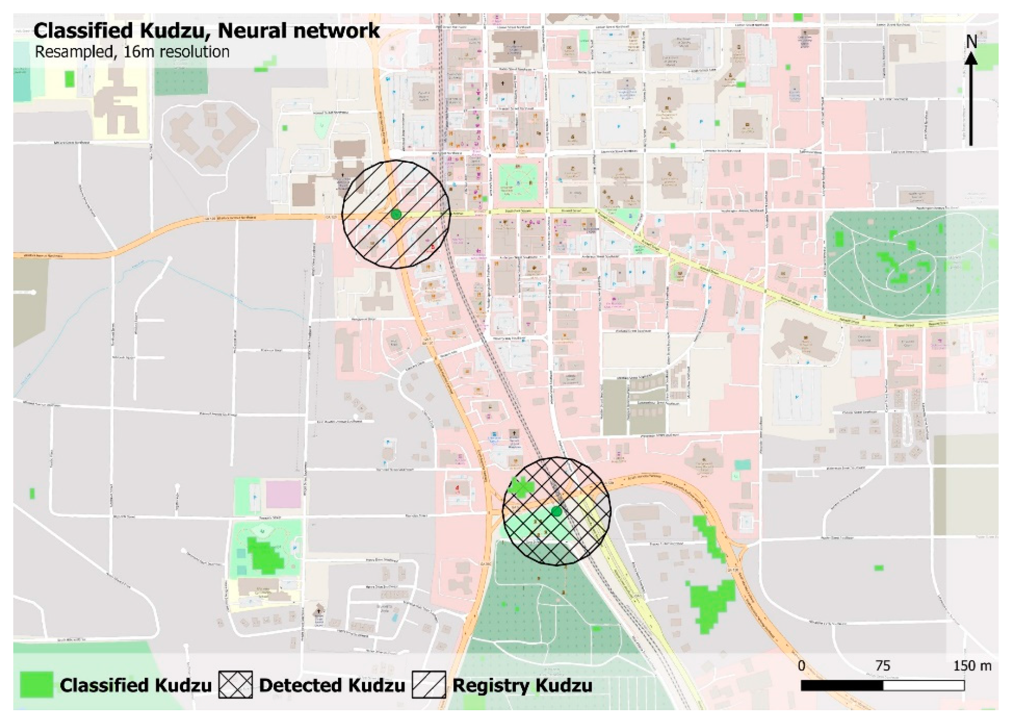
The registered point, from the EDDmaps database, might be placed in a road intersection, while the observed Kudzu was seen down the street. The reason for this lies in the fact that the requirements for the registered areas were lenient in EDDmaps and this leads to some inaccuracy [30]. This was addressed by assigning a 100-m buffer to each point. Once these adjustments had been implemented, it was possible to count how many external points had been classified as Kudzu. An example of the geography can be seen in Figure 2.
The hashed circles are the buffers calculated around the central EDDmaps point. If a buffer intersected with an area of classified Kudzu, this was counted as an accurate classification, and is shown as “Detected Kudzu”. Points that the classification failed to identify are the “Registry Kudzu”.

3. Results

By having four image stacks with five algorithms to run on each stack, a total of 20 results could be evaluated.
The results were evaluated against six different accuracy measures:
  • Accuracy–Percentage of samples correctly classified
  • Kappa–Accuracy accounted for being correct by chance
  • Lower Classification Accuracy–Lower classification accuracy bounds of the 95% confidence interval
  • Upper Classification Accuracy–Upper classification accuracy bounds of the 95% confidence interval
  • Null Accuracy–Expected accuracy of predicting the most frequent class
  • McNemarPValue–Describes which class the model is best as predicting, where 1 is equal performance on both classes, and 0 is superior performance on one class.
After examining the results above, it is evident that given the same data and tuning circumstances some classifiers outperform others when given the same predictors. Some perform well even with very few predictors such as the NN, while others such as the NB classifier cannot function under the same restricted circumstances. The most interesting conclusions, which can be drawn from the overall accuracy results, can be seen in the Kappa, and to some extent in the accuracy values. The Kappa value is the most indicative of the change in performance between the models, as the accuracy value is mostly decided by how many of the not Kudzu pixels are correctly classified.
The multispectral results generally performed well when examining the overall results. There were some substantial differences in the Kappa values with neural network and SVM being the best performers. The overall accuracy is not the best descriptor in this case, since the non-Kudzu class is very dominant and easily identifiable. This is also the reason why it does not change very much between classifiers. The accuracy results from the hyper-spectral data are much more varied than the multi-spectral data. The algorithm that performs the best is the neural network with high accuracy and Kappa values despite the low number of predictors. The low number of predictors is generally what inhibits the other algorithms the most.
In the context of this study, the P values which should be examined further are the values approaching 0. Such a low value would indicate that the classifier has some underlying reason to classify one class much more effectively than the other. As seen in Table 3, a couple of the classifiers have very low P values. In particular, the random forest algorithm is noteworthy, since it produces a P value of 0 when using multi-spectral predictors and P value of 1 when using the hyper-spectral data. In the hyperspectral modeling results, the McNemar P-value indicates that the RF and SVM algorithms are balanced in their classification of the two classes and both NN and NB algorithms are better at classifying one class by a small margin.
The analysis above indicates that for some classifiers, the underlying data and number of predictors hold a lot of importance. More predictors would in most cases increase the performance of the classifiers. This is examined in the next section where the multispectral and hyperspectral data is combined, which means additional data for the PCA and a higher number of predictors. It is difficult to make any general recommendation since the combined results vary a lot across algorithms. The neural network does not perform very well on the smaller grid, but improves a lot in the Kappa measure when performed on the 16 m grid. The opposite is true for SVM, which is better on the smaller grid. The algorithm, which seems to perform well regardless of changes to the underlying factors, is the random forest algorithm. This could be due to the nature of random forest by generating vast decision trees that allow for smoothing the results.
In combining the data sources, the algorithms once again perform better. It is difficult to draw any conclusions from the poor results seen with regards to the SVM algorithm, which was applied to the AVIRIS data in Table 3 besides the fact that the algorithm is not suited to work with only two variables. It is interesting to note that the algorithm with the combined data outperforms the scenario with multi-temporal data, even though the combined data reduces to seven variables as compared to the multi-temporal scenario with ten variables. The reason for this might be that when introducing the 56 extra bands to the 224 bands, the combination of bands that make up the 95% threshold might negate some of the high correlation that the AVIRIS data set holds. The Sentinel-2 bands are a lot less correlated than AVIRIS, resolving in the need of seven bands instead of 2. This highlights that the algorithm only becomes inhibited at extremely low dimensionality and that the seven variables from the combined data sources hold more exact information that can be used to construct the model.
When comparing overall statistics from the combined and resampled stacks with the Sentinel-2 or AVIRIS stacks, an improvement is seen across all metrics, the most obvious one being the increase in Kappa values. It is interesting to note that the multi-temporal results are comparable to the results from the combined data. The Sentinel-2 data by itself results in a mean Kappa value of 0.866 and shows a steady performance across all algorithms, with more varied performance when the data is combined. The four confusion matrices below show the highlighted classifiers in Table 3. These were the best performing classifiers of each image stack.
Examining the confusion matrices, it is obvious that in the case of multi-spectral classification, as seen in Table 4, the Kudzu class is mistaken for no-Kudzu much more often than the other way around. For the hyperspectral data, as seen in Table 4, the misclassification is much more balanced. This would indicate a general lack of performance in the classifier, rather than the bias towards one class seen in the multi-spectral data. It is noticeable that the confusion matrices for the resampled data are identical. This is coincidental, but not unlikely as all the accuracies are fairly even, as seen in Table 3.
The number of predictors was the same for both the different resampling methods and therefore the predictors can no longer be the deciding factor for the different algorithms performing differently between the two tests. With regards to resampling, the model yields a better result when data are resampled from 16.6 m to 10 m. When the grids are not divisible, data will be lost regardless of the sampling direction. The results presented in Table 3 indicates that down-sampling keeps the data integrity to a higher degree than up-sampling.

External Validation

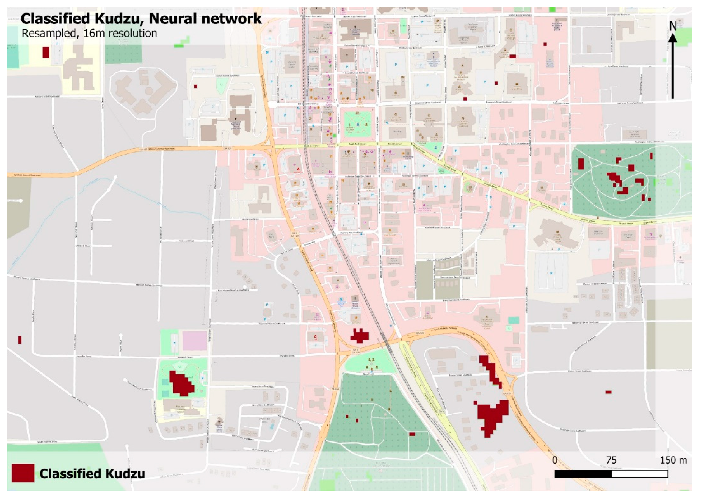
The above results are the model evaluations of its own performance, and have a lower correlation with the degree that the results are consistent with the real world. The external validation presented here provide an indication of this. External validation was carried out on four generated predictions, which were produced using the neural network algorithm. This resulted in the four raster files, which classified the area of interest into Kudzu (1) and no-Kudzu (0) as shown in Figure 3. The predictions can be seen in Supplementary Materials A.2.
Table 5 shows the results from measuring the performance of four classifications all using the neural network algorithm. The only difference lies in the grid underneath.
Considerably lower accuracy is seen for all predictions, than what was observed in earlier accuracy estimates. The results could be improved upon in several ways, which will be described in Section 4. The general trend shown by the result of the external validation does, however, line up with the previous results. The preprocessed AVIRIS data returns the poorest result and the combined and resampled data produces the most accurate results. It should be noted that the number of points used for the external validation is low and this determines the reliability of the results.

Expanded Area Classification

To verify the utility of the project modeling approach, the classification was expanded to include areas that are outside of the bounds used for producing the model. Since there is a lack of available AVIRIS data in this new area and because the findings presented in Table 3, all point to the multispectral data performing well, it was decided that this final classification would solely utilize multispectral data.
The expanded AOI is defined by the rectangular bounds of the original AOI. The classification was performed using the same methodology as in the initial AOI, using a neural network classifier. Furthermore, the classification was verified using the buffer method described in the previous section, using 100 m buffers. The geographic situation can be seen in Figure 4.
When applying the buffers and counting the detected Kudzu as was illustrated in Figure 2, the prediction correctly detects 163 out of a total 205 points, including the 55 locations, which were used in the original AOI. This is a satisfactory result with an accuracy rate of 79.5%.

4. Discussion

The following discussion brings up a handful of relevant points, which were not implemented in the presented solution. These could be included in future studies.

4.1. Are the Achieved Results Useful? What Would Their Purpose be and What Kind of Appropriate Action Should be Taken?

The achieved result both sheds light on the performance of different algorithms and on the impact that different data has on the classification results. From the comparative analysis, some general conclusions can be drawn, which could be of assistance when one needs to decide upon a fitting algorithm for classification.
With regards to achieving acceptable results, it would seem that hyperspectral data is not necessarily a requirement. The classification algorithms performed well on the multi-temporal Sentinel-2 data and this would indicate that for some applications the freely available remote-sensing products could be sufficient, which would allow for a cheaper process with regards to the data collection. While it is true that the hyper-spectral data does contribute to a better result, it also increases the workload in data processing and computation resources. It is therefore arguable whether it is worth including in all cases, but should be seriously considered as a resource when it is available.
As a method for reducing the dimensionality of data, the principal component analysis makes sense from a conceptual viewpoint. Its impact on data modeling varies greatly however, and therefore one should be cautious when applying PCA. In Table 3, it can be seen how some algorithms such as BLR was performing very poorly with dimensionality reduction, while other algorithms, such as NN, performed well regardless of whether it was used or not. To examine this further, three new models have been generated without PCA. This was done using only hyper-spectral data and just for the three algorithms, which performed poorly. The results of this can be seen in Table 6.
All three algorithms exhibit the opposite tendency of previous models in that they are better at identifying Kudzu than the no-Kudzu class. Because of limited resources, it has not been possible to perform an external validation of the results of these models, but it would be interesting to examine them further, possibly in a future study.
The reason for the poor performance on the AVIRIS data with PCA most likely stems from the fact that despite many of the bands being correlated, they do not all assist in detecting Kudzu. It would therefore have been prudent to remove many of the bands that do not have much impact, such as a large number of optical bands, since these are highly correlated. These optical bands cover a large part of the variance in the data, and when PCA is performed on the data the threshold for 95% variance is quickly fulfilled, therefore only making a few components necessary in the model. Removing these bands before using PCA might yield a better result, as there might be more bands needed to reach the threshold, and therefore a need for additional principal components.
One last issue, that should be noted is the distribution of the validation data points. These data points have a clustered structure and this becomes a problem when the data is split into training and testing partitions. Figure 5 highlights the problem.
Once the data was split using the 70/30 percent split, the testing points were within the bounds of the training points. This meant that the training data passed to model made the model very good at modeling the Kudzu clusters and their bounds in the immediate surroundings of the training data. These clusters, which were modeled very well, contained the 30% testing data and resulted in very accurate results, which should be viewed as being somewhat misleading. Having testing data points which were truly separate from the training data is a much more realistic way of evaluating the modeling performance. This was also the reason for using the implemented external validation methodology, which was described in Section 2.4 since it circumvents this clustering problem.
Another approach which is speculated to improve results would be to iterate on the predicted results using newly validated occurrences in training future models.

4.2. Could this Approach be Used with Different Plants or in Different Areas?

As seen in the external validation (see Section 2.4), the modeling was successful in predicting Kudzu occurrences. This indicates that the model could be used with success in other geographic areas and similar results should be expected. One factor that could mislead the model is that as the geographic extent changes across large distances Kudzu might have different spectral signatures, which could decrease model performance or increase the number of false positives. This change could originate in the different yearly cycle as climate changes from state to state or other plants which are similar to Kudzu begin appearing. One should therefore be cautious at shifting too much from the geography of the training area, as the other regions have different ecosystems. If a more widespread application was to be made, this issue could be overcome by including training data from several different areas.

5. Conclusions

In concluding the study, the proposed research questions will be answered based on the results and considerations which were presented.
Research question 1:
How accurately can Kudzu be classified using different machine learning algorithms on a Sentinel-2 multispectral image versus AVIRIS hyperspectral data?
The classification results are difficult to compare and conclude upon, given the unintended impact the PCA had on the hyperspectral data. Regardless, the multispectral data proved sufficient in mapping Kudzu accurately, which was presented in Section 3. The actual algorithm used for the five predictions and cross-comparison purposes, was the neural network model, which was among the top performers, as indicated in Section 3. Other algorithms might have performed similarly on the multispectral data and achieved around 60%–80% accuracy if they were to be externally validated. This is supported by the model performances for the best algorithms, which are shown in Table 3.
The hyperspectral data performed poorly because of PCA being applied in a suboptimal manner. The results were, despite this, useful and in the case of the neural network algorithm, the results were comparable to its multispectral counterpart, even with the very low number of predictors. The multispectral model had an internal Kappa value of 0.91, which is only slightly higher than the hyperspectral kappa of 0.90. This indicates that using hyperspectral data without PCA would have outperformed the multispectral approach by some margin.
Research question 2:
What differences will be seen using several multispectral images from around the year as compared to results from using a single hyperspectral image?
A significant difference between the results from the two data sources was observed when treating them using the same methodology, which included PCA. The consequence was that algorithm accuracy was more stable for the multispectral data than for hyperspectral data, since the reliability of some of the models depended a lot on the number of predictors. Here, the multispectral classification yielded better results than the hyperspectral, due to the fact that AVIRIS was reduced to only two predictors. The general conclusions that can be drawn from the test was that the multispectral classification yields satisfactory results and that hyperspectral data may not be necessary to perform accurate classification.
Research question 3:
How does combining multi- and hyperspectral data affect the overall accuracy and does resampling have any influence on the result?
The best results were achieved using a combination of the two data sources. This was seen in Table 5, where the multispectral and hyperspectral data resampled to 16.6 m achieved an external accuracy of 66%. This is however only marginally better than using just multispectral data for the classification, which reached 64% external accuracy. There is seemingly some variance as to how well the algorithms perform when applied to differently resampled data. Therefore, resampling should be tested for the chosen algorithm, as no general rule can be determined.

Guidelines and Recommendations

When performing dimensionality reduction, it is recommended to begin with feature selection by using variable importance methods. Secondly, performing a PCA is recommended. In this context, it is essential to consider how many components should be included. This number is dependent on the chosen algorithm.
As seen in this article, the results from the AVIRIS test returned poor results, but others should not refrain from using the product, since it holds potential as shown in Section 4. This study uses the product in a suboptimal manner. Firstly, one side of the image had a high degree of cloud cover, which was not dealt with and consequently affected the result. Secondly, all bands were used on the AVIRIS product, and a lot of these bands were optical bands, which could have been left out, as they did not contribute any more to the result than just having one of each band would have. Following these guidelines, it is expected that including AVIRIS data would contribute to a marked improvement in accuracy, compared to what was achieved in this study.

Supplementary Materials

The following are available online at https://www.mdpi.com/2071-1050/12/9/3544/s1, Appendix A.1: Executable in RStudio. Includes full R code used for the modeling as well as a RStudio workspace and a zip-folder containing validation data in .shp-format. Appendix A.2: Output raster files in .tif-format of all predictions made using Neural Network (georeferenced, WGS84). Additional descriptions can be found in the README.txt.

Author Contributions

Conceptualization, J.J.A.; Supervision, J.J.A.; Writing—original draft, T.J., F.S.H., M.S.A. and P.H.P.; Writing—review & editing, J.J.A., T.J., F.S.H. All authors have read and agreed to the published version of the manuscript.

Funding

This research received no external funding.

Conflicts of Interest

The authors declare no conflict of interest.

References

  1. Order, E.P. Executive Order 13112 of February 3, 1999: Invasive Species. Fed. Regist. 1999, 64, 6183–6186. [Google Scholar]
  2. Invasive Species Advisory Committee. Invasive Species Definition Clarification and Guidance. 2006. Available online: https://www.doi.gov/sites/doi.gov/files/uploads/isac_definitions_white_paper_rev.pdf (accessed on 1 April 2019).
  3. Walsh, J.R.; Carpenter, S.R.; Vander Zanden, M.J. Invasive species triggers a massive loss of ecosystem services through a trophic cascade. Proc. Natl. Acad. Sci. USA 2016, 113, 4081–4085. [Google Scholar]
  4. Invasive Species Working Group. Economic impact of invasive species in the pacific Northwest economic region. 2012. Available online: https://www.river-management.org/assets/docs/Listserve/economicimpactspnwer.pdf (accessed on 1 April 2019).
  5. Pimentel, D.; Zuniga, R.; Morrison, D. Update on the environmental and economic costs associated with alien-invasive species in the United States. Ecol. Econ. 2005, 52, 273–288. [Google Scholar]
  6. Bradley, B.A. Remote detection of invasive plants: A review of spectral, textural and phenological approaches. Biol. Invasions 2014, 16, 1411–1425. [Google Scholar]
  7. Xie, Y.; Sha, Z.; Yu, M. Remote sensing imagery in vegetation mapping: A review. J. Plant Ecol. 2008, 1, 9–23. [Google Scholar] [CrossRef]
  8. Stewart, M.A. Cultivating Kudzu: The Soil Conservation Service and the Kudzu Distribution Program. Ga. Hist. Q. 1997, 81, 151. [Google Scholar]
  9. Vaz, A.S.; Alcaraz-Segura, D.; Campos, J.C.; Vicente, J.R.; Honrado, J.P. Managing plant invasions through the lens of remote sensing: A review of progress and the way forward. Sci. Total Environ. 2018, 642, 1328–1339. [Google Scholar] [CrossRef] [PubMed]
  10. Department of Agriculture and Fisheries Biosecurity Queensland. Invasive plant risk assessment: Kudzu Pueraria montana var. lobata 2. 2016. Available online: https://www.daf.qld.gov.au/__data/assets/pdf_file/0004/74137/IPA-Kudzu-Risk-Assessment.pdf (accessed on 15 April 2019).
  11. Ismail, R.; Mutanga, O.; Peerbhay, K. The identification and remote detection of alien invasive plants in commercial forests: An Overview. South Afr. J. Geomat. 2016, 5, 49–67. [Google Scholar] [CrossRef] [Green Version]
  12. Skowronek, S.; Ewald, M.; Isermann, M.; Van De Kerchove, R.; Lenoir, J.; Aerts, R.; Warrie, J.; Hattab, T.; Honnay, O.; Schmidtlein, S.; et al. Mapping an invasive bryophyte species using hyperspectral remote sensing data. Biol. Invasions 2017, 19, 239–254. [Google Scholar] [CrossRef]
  13. Vane, G.; Green, R.O.; Chrien, T.G.; Enmark, H.T.; Hansen, E.G.; Porter, W.M. The airborne visible/infrared imaging spectrometer (AVIRIS). Remote Sens. Environ. 1993, 44, 127–143. [Google Scholar] [CrossRef]
  14. Wang, Z.; Schaaf, C.B.; Sun, Q.; Kim, J.; Erb, A.M.; Gao, F.; Román, M.O.; Yang, Y.; Petroy, S.; Taylor, J.R.; et al. Monitoring land surface albedo and vegetation dynamics using high spatial and temporal resolution synthetic time series from Landsat and the MODIS BRDF/NBAR/albedo product. Int. J. Appl. Earth Obs. Geoinf. 2017, 59, 104–117. [Google Scholar] [CrossRef]
  15. McIntyre, D.L. Application of High Resolution Remote Sensing to Detect and Map the Pasture Weed Paterson’s Curse (Echium Plantagineum) in Western Australia. Ph.D. Thesis, Curtin University, Perth, Australia, 2015. [Google Scholar]
  16. Campbell, J.B.; Wynne, R.H. Introduction to Remote Sensing; Guilford Press: New York, NY, USA, 2011. [Google Scholar]
  17. Paz-Kagan, T.; Silver, M.; Panov, N.; Karnieli, A. Multispectral Approach for Identifying Invasive Plant Species Based on Flowering Phenology Characteristics. Remote Sens. 2019, 11, 953. [Google Scholar] [CrossRef] [Green Version]
  18. Satellite Imaging Corporation. Sentinel-2A Satellite Sensor (10 m). 2019. Available online: https://www.satimagingcorp.com/satellite-sensors/other-satellite-sensors/sentinel-2a/ (accessed on 2 May 2019).
  19. NASA Jet Propulsion Laboratory. AVIRIS. 2019. Available online: https://aviris.jpl.nasa.gov/ (accessed on 29 April 2019).
  20. The University of Georgia. EDDMapS—About. 2019. Available online: https://www.eddmaps.org/about/ (accessed on 17 April 2019).
  21. Bungaro, L. How to Evaluate your Machine Learning Model. 2018. Available online: https://medium.com/coinmonks/debugging-a-learning-algorithm-ef7c16936864 (accessed on 17 May 2019).
  22. Donges, N. The Random Forest Algorithm. 2020. Available online: https://builtin.com/data-science/random-forest-algorithm (accessed on 26 February 2020).
  23. Leon, K. Making a Simple Neural Network. 2017. Available online: https://becominghuman.ai/making-a-simple-neural-network-2ea1de81ec20 (accessed on 13 May 2019).
  24. Ray, S. Understanding Support Vector Machine Algorithm from Examples (along with Code). 2017. Available online: https://www.analyticsvidhya.com/blog/2017/09/understaing-support-vector-machine-example-code/ (accessed on 22 May 2019).
  25. Gandhi, R. Naive Bayes Classifier. 2018. Available online: https://towardsdatascience.com/naive-bayes-classifier-81d512f50a7c (accessed on 29 May 2019).
  26. Subasi, C. LOGISTIC REGRESSION CLASSIFIER. 2019. Available online: https://towardsdatascience.com/logistic-regression-classifier-8583e0c3cf9 (accessed on 29 May 2019).
  27. James, G.; Witten, D.; Hastie, D.; Tibshirani, R. An Introduction to Statistical Learning with Application in R; Springer: Berlin, Germany, 2013. [Google Scholar]
  28. Scikit-learn. Cross-validation: Evaluating estimator performance. 2019. Available online: https://scikit-learn.org/stable/modules/cross_validation.html (accessed on 14 May 2019).
  29. Tipping, M.E.; Bishop, C.M. Mixtures of probabilistic principal component analyzers. Neural Comput. 1999, 11, 443–482. [Google Scholar] [CrossRef] [PubMed]
  30. Bargeron, C.T.; Moorhead, D.J. EDDMapS—Early detection and distribution mapping system for the southeast exotic pest plant council. Wildland Weeds 2007, 10, 4–8. [Google Scholar]
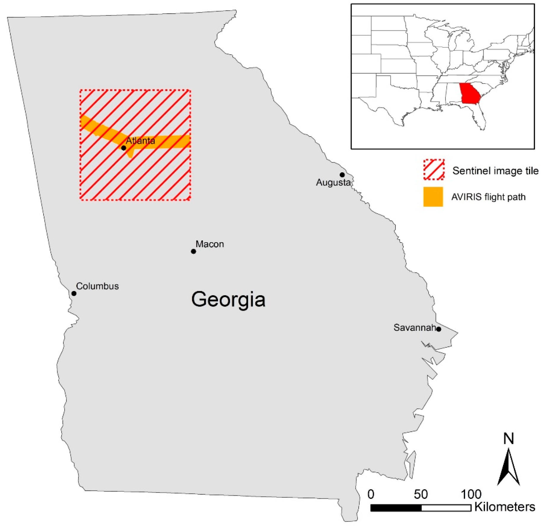
Figure 1. Area of interest defined by the bounds of the Sentinel-2 image and the flight path of airborne visible/infrared imaging spectrometer (AVIRIS) in Georgia.
Sustainability 12 03544 g001
Figure 2. Classified Kudzu pixels, detected EDDmaps points and registry EDDmaps points.
Sustainability 12 03544 g002
Figure 3. Classified Kudzu pixels (1) clustered in an urban environment.
Sustainability 12 03544 g003
Figure 4. The expanded AOI surrounding the original AOI.
Sustainability 12 03544 g004
Figure 5. Issue when splitting the data into training and testing partitions.
Sustainability 12 03544 g005
Table 1. Images capturing periods per season.
SeasonStartEnd
Spring1 April 201729 May 2017
Summer1 June 201701 September 2017
Autumn1 October 201729 November 2017
Winter12 December 201707 February 2018
Table 2. Image stacking summary.
Stack# of BandsBandsResolution
Sentinel-256 *2, 3, 4, 5, 6, 7, 8, 8a, 11, 12, SAVI & 3x Tasseled cap10 & 20 m
AVIRIS224All16.6 m
Resample (down)280Sentinel-2 + AVIRIS10 m
Resample (up)280Sentinel-2 + AVIRIS16.6 m
* Combining imagery from four seasons, resulting in 4 × 14 bands.
Table 3. Accuracy statistics from running the five algorithms on the four sets of stacked images. Best performing algorithm shown in bold.
Image StackClassifierAcc.KappaAcc. LowerAcc. UpperAcc. NullMcNemarPValue
Sentinel-2 Multispectral Resolution: 10 mBLR0.960.830.940.970.850.17
NB0.950.800.930.960.830.00
NN0.960.860.940.970.830.12
RF0.980.910.960.990.830.01
SVM0.980.950.970.990.830.75
AVIRIS
Hyperspectral
Resolution: 16.6 m
BLR0.940.720.920.960.860.00
NB0.870.510.84 0.900.830.28
NN0.970.900.960.980.830.36
RF0.960.850.940.970.831.00
SVM0.920.700.890.940.831.00
Resample (down) Resolution: 10 mBLR0.960.830.940.970.850.17
NB0.950.800.930.960.830.00
NN0.960.860.940.970.830.12
RF0.980.910.960.990.830.01
SVM0.980.950.970.990.830.75
Resample (up)
Resolution: 16.6 m
BLR0.950.820.930.970.841.00
NB0.950.820.930.970.930.01
NN0.980.950.970.990.830.75
RF0.980.910.960.990.830.01
SVM0.970.890.950.980.830.01
Table 4. Confusion Matrices of the best performing algorithms.
Image StackClassifierConfusion MatrixError 1Error 2Acc. 1Acc. 2
Sentinel-2 Class01
MultispectralSVM054295510.0090.0160.9910.984
Resolution: 10 m 151001050.0830.0480.9170.952
total547109656
AVIRIS Class01
HyperspectralNN053575420.0220.0130.9780.987
Resolution: 16.6 m 1121021140.0640.1050.9360.895
total547109656
Resampled (up) Class01
Resolution: 10 mSVM054145450.0110.0070.9890.993
161051110.0370.0540.9630.946
total547109656
Resampled (down) Class01
Resolution: 16.6 mNN054145450.0110.0070.9890.993
161051110.0370.0540.9630.946
total547109656
Error 1: Omission Error, Error 2: Commission Error, Acc. 1: Producer accuracy, Acc. 2: User accuracy.
Table 5. Compared accuracies in predicting observed Kudzu locations across different data sources.
GridRegistry PointsDetected PointsAccuracy
Sentinel553564%
AVIRIS551018%
Combined, 10 m553360%
Combined, 16 m553666%
Table 6. Testing the three revised algorithms, without PCA, using hyperspectral data. 0 = Not Kudzu, 1 = Kudzu.
Testing the BLR algorithm without PCA, using only hyper-spectral data
Class01 Omission e.Commission e.Producer acc.User acc.
052935320.0130.0060.9870.994
171031100.0280.0640.9720.936
total536106642
Testing the NB algorithm without PCA, using only hyper-spectral data
Class01 Omission e.Commission e.Producer acc.User acc.
0441414820.1920.0850.8080.915
1105681730.3760.6070.6240.393
total546109655
Testing the SVM algorithm without PCA, using only hyper-spectral data
Class01 Omission e.Commission e.Producer acc.User acc.
054305430.0050.0000.9951.000
131091120.0000.0271.0000.973
total546109655