Evolution of Ecological Security in the Tableland Region of the Chinese Loess Plateau Using a Remote-Sensing-Based Index

Abstract

Maintaining optimal ecological security is a serious issue in the Chinese Loess Plateau (CLP). Remote sensing ecological indexes (RSEI) of three main tableland regions of the CLP were calculated based on spectral information provided by remote sensing imaging satellites between 2000 and 2018. We were able to use RSEI values to systematically evaluate the temporal and spatial variation in the regional ecological environment and determine the influential factors that mainly associated with these changes. The results showed that between 2000 and 2018, the ecological environment improved, remained stable, and deteriorated, respectively, in the Gansu, Shaanxi, and Shanxi tablelands. Regions with poor or fair RSEIs were concentrated around the main river basins, while regions with moderate RSEIs were associated with poor ecological conditions and poor areas. The significant spatiotemporal variation in RSEI indicates that the ecological system in this region is relatively fragile. We also observed that natural factors such as the temperature, potential evapotranspiration, and precipitation had the greatest influence on the overall ecological quality. The rapid increase in the regional population and human activity played an important role in the variation in the regional RSEI. This research will provide important information on controlling regional soil erosion and ecological restoration in the CLP.

1. Introduction

The Chinese Loess Plateau (CLP) is located at the junction of a monsoonal and an arid region, where the climate is arid and the ecosystem is fragile. It covers an extensive area, accounting for approximately 6.6% of the land in China, and accommodates and sustains 8.5% of the Chinese population [1,2]. However, serious soil erosion means that the ecological system of the CLP is facing pressure from the sharp decrease in forests, decreased comprehensive land productivity, and desertification, among other issues, thereby threatening regional ecological security [2,3]. The gully region of the CLP, the most productive crop and agricultural area in the CLP, is now facing a serious ecological security issue due to the shrinking of the tableland. This also causes natural disasters and an inevitable restriction on economic development. Therefore, the timely and rapid monitoring of ecological and environmental changes in areas subject to soil and water loss has become a focus for researchers and the concerned government departments.

Remote sensing methods, particularly aerial photography and satellite imaging, are unique in their ability to record a variety of spatial and temporal data in a comprehensive manner and over wide surfaces; they have proved effective for a variety of applications [4]. Remote sensing has been successfully applied in the last few years as a tool for ecological monitoring, particularly for the evaluation of ecosystems including forests [5], grasslands [6], urban areas [7], and rivers [8], allowing the remote evaluation of the environment through generalized quality indices. Many countries have conducted large-scale ecological monitoring by applying remote sensing technology. The Chinese government is among them; it conducted a nationwide remote-sensing-based ecological assessment from 2000 to 2010 [9]. Similar studies have also been carried out in Europe, the United States, and other regions [10,11,12,13]. A number of single remote sensing indices have been created to quantify ecological status. The normalized different vegetation index (NDVI) is the most widely utilized single indicator and was adopted in ecological monitoring studies of grasslands, forests, and farmland [1,10,14]. Ivits et al. [10] used SPOT NDVI data to analyze the seasonal characteristics of vegetation cover and monitored the suitability of farmland bird habitats. Similar single remote-sensing-based ecological vegetation indexes include the enhanced vegetation index (EVI), permanent vegetation fraction (PVF), and hyperspectral flower index (HFI). Land surface temperature (LST) retrieved from remote sensing thermal imagery can evaluate the expansion of urban areas and ground temperature measurements, allowing for the estimation of changes in the terrestrial thermal environment [15,16,17].

This single-index method can well reflect the variation of natural environmental factors, such as the land surface temperature (using LST) and the land surface phenology (NDVI); it is difficult to comprehensively reflect the combined effects of multiple natural environmental factors [9]. Ecological environment is a complex system, whose variation is controlled by the natural environmental factors (such as temperature, moisture condition, vegetation cover, etc.) and the human factors (architecture, human activities, etc.) [9]. The single index is limited because it only considers one of the numerous influencing factors that interact in the evolution of an ecological system; in natural environments, a visible change often conceals complex dynamics of influences and effects. Aggregated remote-sensing-based multi-indexes have more advantages than single ones. A multi-index can monitor ecological status using several metrics such that many features related to ecological conditions can be identified [9]. Therefore, it is necessary to develop a multi-index monitoring strategy that can comprehensively evaluate variations in ecosystems that can allow the implementation of effective strategies for controlling different natural events. For instance, Tiner [18] developed a multi-index (by integrating habitat disturbance and habitat extent indices) and applied it well to evaluate the environmental variation of the natural habitat of a watershed. The MODIS global disturbance index (MGDI), which combines both the MODIS enhanced vegetation index (EVI) and LST products, is an efficient method to map regular large-scale wildfires [19]. The frequently used forest disturbance index (DI), which combines three components of tasseled cap transformation of remote sensing data, is an efficient multi-index that is widely used to evaluate the characteristics of forest ecosystems [20]. Rhee et al. [21] used three indicators—LST, NDVI, and precipitation data from the Tropical Rainfall Measuring Mission satellite—to develop the scaled drought condition index (SDCI), and applied it to regional drought assessment. The remote sensing ecological index (RSEI), an efficient and useful ecological evaluation index [22], accounts for the variation in multiple environmental parameters, thereby making it a potential candidate with which to quantitatively analyze and evaluate local ecological recovery in China, particularly in areas subject to soil and water loss. Researchers have assessed the validity of the RSEI in different regions of the country, employing it to evaluate changes in a red-soil area in south China [23], a black-soil area in northeast China [24], and pastoral farming crops [25]. However, there are relatively few studies that report the evaluation of ecological conditions in the tableland regions of the CLP, which are subject to soil and water loss. A few select studies on the ecological assessment of the CLP are based on a single indicator or were only conducted by modeling [26,27,28].

The ecological environment of the tableland of the CLP is facing great challenges due to the influence of urban expansion, population increase, climate change, and serious soil erosion [2]. Several studies have indicated that climate change caused an increase in the average annual temperatures of the CLP, which resulted in an alarming increase in water evaporation and, in turn, in the frequency of droughts [1,29,30]. Moreover, the larger regional precipitation fluctuation and the increasing rainfall erosivity resulted in the risk of soil and water loss in this aggravated region. Since 1980, the CLP region has been suffering from severe soil erosion caused by adverse environmental conditions (high-intensity storms, in particular) and intensified human activity (e.g., unorganized coal mining and overgrazing). The average annual soil erosion rate is more than 3000 t km⁻² year⁻¹ and inevitably results in a rapid shrinking of the Loess tableland [1,21,22,23,24,25,26,27,28,29,30,31,32]. This serious land degradation and desertification caused by soil and water loss has caused increasingly severe environmental and socioeconomic problems for the CLP region [26]. To prevent the negative effects of an excessively degraded environment, the Chinese government implemented large-scale conservation plans—including the Shelterbelt program, slope stability improvement programs, the joint governance of gullies and slopes, comprehensive management of small watersheds, and the Great Green Program (GGP)—beginning in 2000 [33]. However, the impact of these large-scale conservation programs on the regional ecosystem is still unclear [2], and no precise information will be available until a quantitative evaluation is made of the environmental quality before and after their implementation.

With this perspective, we selected the CLP regions that are mainly monitored for their soil and water loss by the Chinese national soil and water conservation division as our study areas; we then built a remote sensing ecological index (RSEI) to evaluate the development of the ecosystem in the areas, totally based on remote sensing information, and integrated multiple indicators (NDVI, land surface moisture (LSM), normalized difference built-up and bare soil index (NDBSI), and LST). Our goals were the following: (1) To monitor the long-term dynamics of the RSEI in the Loess tableland from 2000 to 2018; (2) to identify the vulnerable regions of the CLP; (3) to determine the environmental controlling factors that mainly impact the RSEI.

The results of this study will not only provide valuable information on the Loess plateau, but also inform the development of strategies for controlling soil and water losses and improving ecological conditions in similar ecosystem areas, including the Loess plateau itself.

2. Study Area and Methods

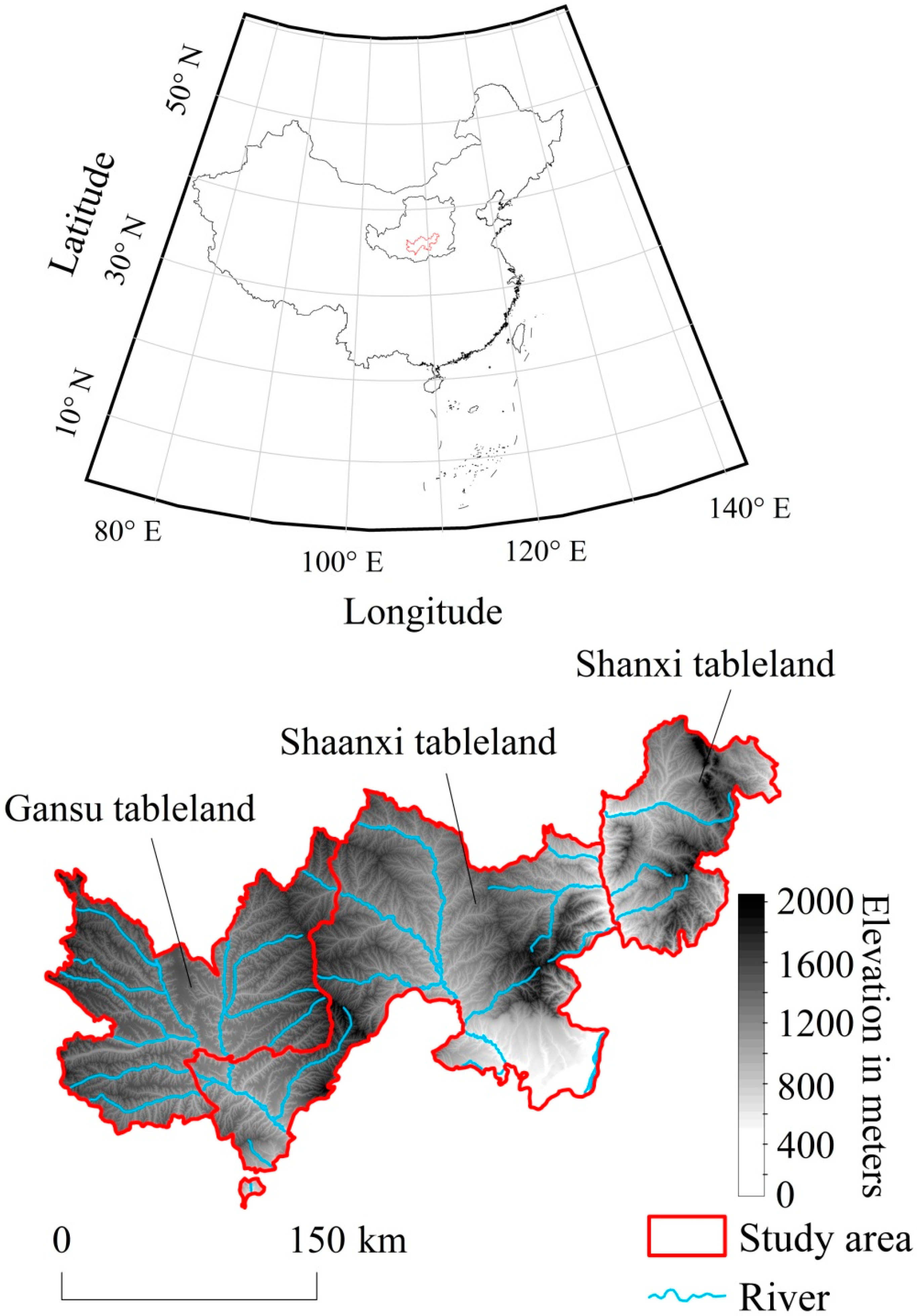
2.1. Study Area

The tableland region of the CLP (a key area protected by the Chinese water conservation project) was selected as the study area, which mainly includes the Gansu tableland region, the Shaanxi tableland region, and the Shanxi tableland region (Figure 1). The study area is located in the south-central part of the CLP (106.7° E–111.7° E, 34.5° N–36.9° N), covering 34 farm- and woodlands of eight cities in the three provinces of Gansu, Shaanxi, and Shanxi, with a total area of around 55,800 km². Topographically, the analyzed portion of the Loess tableland is comprised of different elements, such as sloped plateaus, open and flat plateaus, hills, tableland alternated with gullies, and ravines and gullies that crisscross. It consists of mainly dark Loessal soil and cultivated Loessal soil. The Loess tableland is located in a semi-humid-monsoonal climate zone, which presents a temperate continental climate with four distinct seasons. In this region, the annual temperature oscillated between 8 and 15.6 °C, and the annual rainfall was approximately 450–709 mm, whose temporal distribution was uneven, as 60% of the total precipitations occurred, on average, from July to September. We observed an annual sunshine duration of 2099 to 2900 h, and a leaf abscission period of 156 to 223 days [2,30,34].

The ecological fragility of this tableland is determined by its unique natural conditions, which result in a constant and alarming soil loss, making this area the most impaired in the whole CLP. In 2017, the fifteen-year national soil and water conservation plan of China approved by the State Council designated the gullies of the CLP as critical elements that require special protection. In order to analyze the ecological condition changes in the Loess tableland more systematically, the study area was divided into the Gansu tableland, the Shaanxi tableland, and the Shanxi tableland.

2.2. Data Sources and Pre-Processing

In our study, the partition and monitoring of the areas of interest were based on provincial boundaries (shapefile) and images obtained from the United States Geological Survey (https://glovis.usgs.gov/) with images Landsat 5 TM (Thematic Mapper) and Landsat 8 OLI (Operational Land Imager). Images acquired in October 2000, 2010, and 2018 were collected and analyzed (

Table 1. Data information for the remote images of the Chinese Loess Plateau (CLP).

Tableland Regions	Path/Row	Data Times	Sensor Types
Gansu tableland	127/035	2000.10.01	TM
		2010.10.20
		2018.10.16	OLI
	127/036	2000.10.01	TM
		2010.10.20
		2018.10.10	OLI
	128/035	2000.10.08	TM
		2010.10.20
		2018.10.12	OLI
	128/036	2000.10.08	TM
		2010.10.20
		2018.10.12	OLI
Shanxi tableland	125/035	2000.10.03	TM
		2010.10.22
		2018.10.26	OLI
	126/034	2000.10.26	TM
		2010.10.26
		2018.10.04	OLI
	126/035	2000.10.26	TM
		2010.10.29
		2018.10.04	OLI
Shaanxi tableland	126/035	2000.10.26	TM
		2010.10.29
		2018.10.04	OLI
	126/036	2000.10.26	TM
		2010.10.13
		2018.10.30	OLI
	127/035	2000.10.01	TM
		2010.10.20
		2018.10.16	OLI
	127/036	2000.10.01	TM
		2010.10.20
		2018.10.26	OLI
	128/036	2000.10.08	TM
		2010.10.20
		2018.10.12	OLI

TM—Thematic Mapper; OLI—Operational Land Imager.

). The images were produced by the Landsat Product Generation System (LPGS) and professionally processed to support georegistration prior to analysis. The required preprocessing was conducted before the RSEI was calculated. First, geometric registration was accomplished using the image-to-image registration method in ENVI 5.3 that is the flagship product of Exelis Visual Information Solutions (Boulder, CO, USA); two sets of images were co-registered and approximately 40 ground control points were resampled according to a polynomial algorithm so that the root mean square errors were less than 0.5 per pixel. One image cannot cover the entire study region well; therefore, mosaic reconstruction was conducted on the images and a seamless mosaic was adopted, using the histogram matching method, to correct regional color in the overlap area. The results were obtained after fuzzing the seamlines. Subset data from region of interesting (ROIs) was selected to clip the result after the mosaic was obtained to produce an image of the study area. During the preprocessing of the datasets, the digit number (DN) values of the multispectral bands were further converted into planetary surface reflectance values [35,36]. The radiometric calibration method was chosen for atmospheric correction to allow conversion of the digit number (DN) values. To reduce the impact of weather and cloud cover, FLAASH atmospheric correction was used to process the data, and sensor parameters were derived from image metadata and NASA (http://atmcorr.gsfc.nasa.gov).

Furthermore, meteorological data including temperature (T), potential evapotranspiration (ET₀), rainfall erosion (R), and precipitation (P) were provided by the China Meteorological Administration (http://data.cma.cn/site/index.html). Gross domestic product (GDP), construction areas (Area), and population (Pop) were obtained from statistical yearbooks of Gansu, Shaaxi, and Shanxi provinces.

2.3. Calculation of Remote Sensing Ecological Index

Many studies have proven that the ecological environment of the CLP is mainly influenced by variations in soil moisture and vegetation [2,26,27,28]. Human activities, especially the expansion of built-up areas, also play a key role, because this can rapidly aggravate land conditions by reducing vegetation coverage and increasing erosion [2,8,29]. Therefore, an official evaluation of the conditions of this ecosystem will require a comprehensive model that will encompass the variation in regional air temperature, relative humidity, vegetation coverage, and the land use/land change (LULCC). We built an index that encompassed the greenness, wetness, dryness, and heat of the ecosystem, as those indicators are often used to evaluate ecological quality [15]. They are well represented by the NDVI given in Equation (1), the LSM given in Equations (2) and (3), the NDBSI given in Equation (4), and the LST given in Equation (7). Accordingly, our RSEI integrated them using principal component analysis (PCA), creating a quick and easy indicator with which to monitor and evaluate the ecological environment of the study area. Before the PCA calculation, the four indicators were packed into a four-band image using the layer stacking method in ENVI 5.3; the Forward PCA Rotation New Statistics Rotate was then used to conduct the PCA. As in previous studies [37,38], we classified RSEI values in five categories (excellent, good, moderate, fair, and poor), each comprising values in equal intervals. This allowed us to divide the RSEI scale into five quality levels—excellent, good, moderate, fair, and poor—at intervals of 0.2.

2.3.1. Normalized Differential Vegetation Index (NDVI)

As a widely used vegetation index, the NDVI can effectively reveal the growth status of vegetation [14]. In fact, plants absorb and re-emit solar radiation in two distinct spectral regions, specifically in the infrared and red regions, which makes it easy for earth observation instruments to monitor plant reflectance. Thus, we chose the NDVI as our greenness indicator; its formula is expressed in Equation (1).

$$\mathrm{NDVI}=\frac{R_{nir}-R_{red}}{R_{nir}+R_{red}}$$

(1)

In this equation, R_red is the reflectance of the near-infrared and R_nir is the red bands, respectively.

2.3.2. Land Surface Moisture (LSM)

The LSM is the index that represents the wetness component (reflecting the moisture of soil, water body, and plant), elaborated by Kauth–Thomas Transformation (K-T Transformation) [38]. The wetness components of TM [39] and OLI [40] correspond to different calculation parameters, and can be computed with the following formulas:

$${\mathrm{LSM}}_{\mathrm{TM}}=0.0315R_{blue}+0.2021R_{green}+0.3102R_{red}+0.1594R_{nir}-0.6706R_{mir1}-0.6109R_{mir2}$$

(2)

$${\mathrm{LSM}}_{\mathrm{OLI}}=0.1511R_{blue}+0.1973R_{green}+0.3283R_{red}+0.3407R_{nir}-0.7117R_{mir1}-0.4559R_{mir2}$$

(3)

where $R_{blue}$, $R_{green}$, $R_{red}$, $R_{nir}$, $R_{mir1},$ and $R_{mir2}$ are the reflectance of the blue, green, red, near-infrared, short-wave range 1, and short-wave range 2 bands, respectively.

2.3.3. Normalized Difference Built-Up and Bare-Soil Index (NDBSI)

The NDBSI combined a soil index (SI) [41] and an anthropic index, the index-based built-up index (IBI) [42], and was used to account for the dryness of the area, with its formula expressed as follows:

$$\mathrm{NDBSI}=\frac{SI+IBI}{2}$$

(4)

$$\mathrm{SI}=\left[\left(R_{mir1}+R_{red}\right)-\left(R_{nir}+R_{blue}\right)\right]/\left[\left(R_{mir1}+R_{red}\right)+\left(R_{nir}+R_{blue}\right)\right]$$

(5)

$$\mathrm{IBI}=\frac{2R_{mir1}/\left(R_{mir1}+R_{nir}\right)-\left[R_{nir}/\left(R_{nir}+R_{red}\right)+R_{green}/\left(R_{green}+R_{mir}1\right)\right]}{2R_{mir1}/\left(R_{mir}1+R_{nir}\right)+\left[R_{nir}/\left(R_{nir}+R_{red}\right)+R_{green}/\left(R_{green}+R_{mir1}\right)\right]}$$

(6)

where $R_{red}$, $R_{blue}$, $R_{green}$, $R_{nir},$ and $R_{mir1}$ are the reflectances of the red band, blue band, green band, near-infrared band, and short-wave infrared band 1, respectively.

2.3.4. Land Surface Temperature (LST)

The land surface temperature was retrieved from the thermal bands of the Landsat images (Band 6 in Landsat TM, and Band 10 in Landsat OLI) and processed using the Radiative Transfer Equation (RTE) algorithm [43,44] to represent the heat indicator. The formula we used to express the RTE algorithm is the following:

$$L_{\lambda }=\left[\epsilon B\left(T_s\right)+\left(1-\epsilon \right)L_{\downarrow }\right]\tau +L_{\uparrow }$$

(7)

where $L_{\lambda }$ is the radiance at the sensor, or Top of Atmosphere (TOA) radiance, $\epsilon$ is the land surface emissivity, $B\left(T_s\right)$ is the blackbody radiance given by Planck’s law for a temperature $T_s$ ($T_s$ = LST), $L_{\downarrow }$ and $L_{\uparrow }$ are the downwelling and upwelling atmospheric radiances, respectively, and $\tau$ is the total atmospheric transmissivity between the land’s surface and the sensor. $B\left(T_s\right)$ was expressed as:

$$B\left(T_s\right)=\left[L_{\lambda }-L_{\uparrow }-\tau \left(1-\epsilon \right)L_{\downarrow }\right]/\tau \epsilon$$

(8)

and $T_s$ was obtained based on Planck’s law:

$$T_s=K_2/ln(K_1/B\left(T_s\right)+1)$$

(9)

where $K_1$ = 607.76 W m⁻² µm⁻¹ sr⁻¹ and $K_2$ = 1260.56 K if obtained from the TM, and $K_1$= 774.89 W m⁻² µm⁻¹ sr⁻¹ and $K_2$ = 1321.08 K for the Thermal Infrared Sensor (TIRS) Band 10. The atmospheric parameters $L_{\uparrow }$, $L_{\downarrow }$, and $\tau$ were acquired from NASA’s website (http://atmcorr.gsfc.nasa.gov/).

2.3.5. Combination of the Indicators

The RSEI was calculated as:

$$\mathrm{RSEI}=\mathrm{PC}1\left[f\left(NDVI,LSM,NDBSI,LST\right)\right]$$

(10)

The formula for reverse processing is:

$$\mathrm{RSEI}=1-\mathrm{PC}1\left[f\left(NDVI,LSM,NDBSI,LST\right)\right]$$

(11)

Since the units and data ranges of the four indicator values were different, normalization had to be performed before generating the RSEI, which resulted in all of the values being in the range 0 to 1. We also needed to normalize the value of the RSEI so that it would range from 0 to 1; from the resulting scale, the closer the value was to 1, the better the ecological quality, and vice versa [38]. The normalized value of the RSEI was calculated as follows:

$${\mathrm{NI}}_{\mathrm{i}}=\frac{I_i-I_{min}}{I_{max}-I_{min}}$$

(12)

where ${\mathrm{NI}}_{\mathrm{i}}$ is the normalized value of a pixel, $I_i$ is the value of a pixel, and $I_{max}$ and $I_{min}$ are the max and min values of a pixel, respectively.

According to previous studies [37,38], we classified RSEI values in five categories (excellent, good, moderate, fair, and poor), each comprised of an equal interval of values. This procedure allowed us to divide the RSEI scale into five quality levels in 0.2 intervals, namely excellent, good, moderate, fair, and poor quality.

2.3.6. Change Vector Analysis

In this paper, the change vector analysis (CVA) method is used to detect the temporal and spatial dynamic changes of the ecological environment in the research area, which can detect the specific changes of RSEI in different years [45,46,47]. CVA is mainly used to calculate the vector change CV of two images; taking the pixels of two images as the basic unit, the basic difference calculation is carried out on the images of two phases to obtain the change vector. The formula is as follows:

$$\mathrm{R}=\left[\begin{array}{c}{\mathrm{r}}_1\\ {\mathrm{r}}_2\\ ⋮\\ {\mathrm{r}}_{\mathrm{i}}\end{array}\right],\mathrm{T}=\left[\begin{array}{c}{\mathrm{t}}_1\\ {\mathrm{t}}_2\\ ⋮\\ {\mathrm{t}}_{\mathrm{i}}\end{array}\right]$$

(13)

$$\Delta \mathrm{E}=\mathrm{R}-\mathrm{T}=\left[\begin{array}{c}{\mathrm{r}}_1-{\mathrm{t}}_1\\ {\mathrm{r}}_2-{\mathrm{r}}_2\\ ⋮\\ {\mathrm{r}}_{\mathrm{i}}-{\mathrm{t}}_{\mathrm{i}}\end{array}\right]$$

(14)

$$\Vert \Delta \mathrm{E}\Vert =\sqrt{{\left({\mathrm{r}}_1-{\mathrm{t}}_1\right)}^2+{\left({\mathrm{r}}_2-{\mathrm{t}}_2\right)}^2+\cdots +{\left({\mathrm{r}}_{\mathrm{i}}-{\mathrm{t}}_{\mathrm{i}}\right)}^2}$$

(15)

where R and T are two RSEI images, i is the number of bands independent of each other that participate in the calculation, $\Delta \mathrm{E}$ is the change vector of two images, and $\Vert \Delta \mathrm{E}\Vert$ is the change magnitude that denotes the total changes between R and T. The greater the $\Vert \Delta \mathrm{E}\Vert$ is, the greater the difference of the two images is. Then, the threshold value is set, and the change region of $\Vert \Delta \mathrm{E}\Vert$ is divided according to the threshold value. If $\Vert \Delta \mathrm{E}\Vert$ is greater than the threshold value, it is the change region; if E is less than the threshold value, it is the unchanged region. The determination method of the threshold value is as follows.

In this study, the Maximum Inter-Class Variance Method or Otsu Method as an adaptive threshold determination method was conducted to determine the change threshold. It divides the image into two categories, namely C₀ and C₁. When the variance between the categories reaches the maximum, the gray level is the best threshold. The mathematical description is as follows: Let the number of image pixels be N, the gray scale range is (0, L), and the number of pixels corresponding to the gray level i is n_i; the probability of its occurrence is:

$$p_i=\frac{n_i}{N}, i=0, 1, 2\cdots , L, {\displaystyle \sum }_{i=0}^L{p}_i=1$$

(16)

The pixels in the image are divided into two types, A and B, according to the gray level threshold t. A is composed of pixels between gray levels (0, t), and B is composed of pixels between gray levels (t + 1, L). The probabilities of A and B are:

$${\omega }_A={\displaystyle \sum }_{i=0}^t{P}_i, {\omega }_B={\displaystyle \sum }_{i=i+1}^L{P}_i=1-{\omega }_A$$

(17)

The average gray values of A and B are:

$${\mu }_A={\displaystyle \sum }_{i=0}^t\frac{i{P}_i}{{\omega }_A}, {\mu }_B={\displaystyle \sum }_{i=t+1}^L\frac{i{P}_i}{{\omega }_B}$$

(18)

The average gray value of the whole image is:

$$\mu ={\omega }_A{\mu }_A+{\omega }_B{\mu }_B$$

(19)

Define the variance between classes as:

$${\sigma }^2={\omega }_A{\left({\mu }_A-\mu \right)}^2+{\omega }_B{\left({\mu }_B-\mu \right)}^2$$

(20)

Parameter t belongs to the range (0, L), and increases in steps of 1 in sequence. When ${\sigma }^2$ is maximum, the corresponding t is the optimal threshold.

3. Results and Discussion

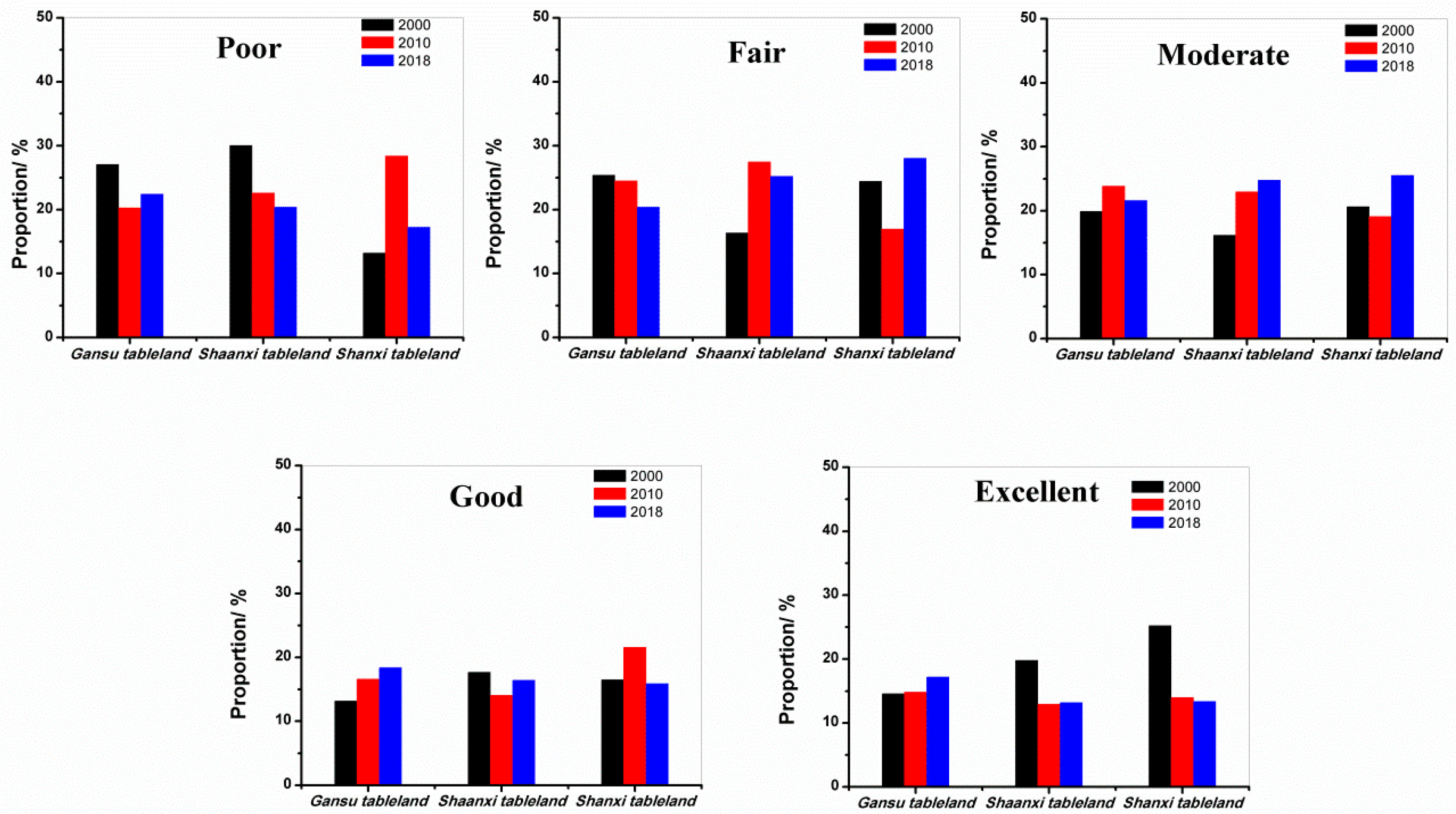
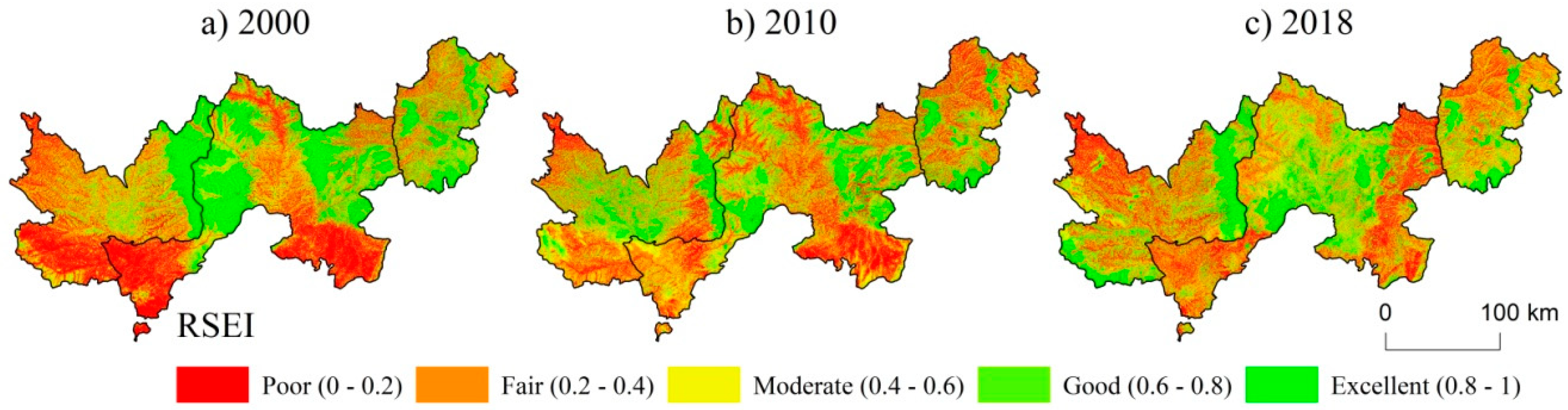
3.1. Ecological Status of the Study Area

We combined the NDVI, LSM, NDBSI, and LST using the PCA method provided in ENVI. The signs of the first principal component (PC1) loadings of LST and NDBSI were the inverse of those of LSM and NDVI (

Table 2. The variation of the four indicators and the remote sensing ecological index (RSEI) during the study period.

Periods	Regions	Types	NDBSI	LST	NDVI	LSM	RSEI
2000	Gansu tableland	Average value	0.62	0.51	0.38	0.48	0.43
		PC1 loading	0.49	0.48	−0.49	−0.54
	Shaanxi tableland	Average value	0.56	0.27	0.31	0.30	0.45
		PC1 loading	−0.52	−0.39	0.55	0.53
	Shanxi tableland	Average value	0.60	0.45	0.60	0.60	0.54
		PC1 loading	0.56	0.42	−0.54	−0.47
2010	Gansu tableland	Average value	0.57	0.75	0.51	0.44	0.46
		PC1 loading	0.57	0.37	−0.58	−0.46
	Shaanxi tableland	Average value	0.63	0.55	0.51	0.47	0.43
		PC1 loading	−0.56	−0.40	0.47	0.56
	Shanxi tableland	Average value	0.72	0.59	0.74	0.64	0.44
		PC1 loading	−0.54	−0.43	0.26	0.67
2018	Gansu tableland	Average value	0.60	0.52	0.49	0.50	0.47
		PC1 loading	0.57	0.38	−0.43	−0.59
	Shaanxi tableland	Average value	0.53	0.69	0.53	0.51	0.45
		PC1 loading	0.58	0.08	−0.53	−0.61
	Shanxi tableland	Average value	0.74	0.54	0.56	0.80	0.46
		PC1 loading	0.67	0.58	−0.25	−0.38

Note: PC1 (first principal component) loading represents the contribution of each indicator to the remote sensing ecological index (RSEI).

), suggesting that the two groups of indicators had opposite effects on the ecology of the study area. We concluded, based on previous studies [9,36], that the LST and NDBSI have negative effects, while LSM and NDVI indicate constructive factors. In general, a larger value of PC1 indicated better ecological quality; however, in some cases, that showed opposite signs compared to the other cases—for example, PC1 loading for the Gansu tableland in 2000; PC1 needed to be processed to make a large negative PC1 value represent good ecological quality (Table 2).

Figure 2 shows the average RSEI values of each tableland from 2000 to 2018. From their comparison, we can see how there was a steady increase in the average RSEI value from 0.43 in 2000 to 0.47 in 2018 in the Gansu tableland. A slightly complex trend, with an initial decrease from 0.45 (2000) to 0.43 (2010), and then an increase back to 0.45 (2018), was observed in the Shaanxi tableland. Finally, a slow and constant decrease from 0.54 (2000) to 0.44 (2010), and then a slight increase to 0.46 (2018), occurred in the Shanxi tableland. This signifies that the ecological environment had improved over time in the Gansu tableland, remained stable in the Shaanxi tableland, and deteriorated in the Shanxi tableland.

Figure 3 shows the spatial distributions of the different quality grades of RSEI on a map, and compares the RSEI levels in 2000, 2010, and 2018, respectively. For the Gansu tableland, the amount of poor and fair values decreased by 6.73% and 0.87%, respectively, between 2000 and 2010. The regions with “poor” and “fair” RSEI were mainly located in the basins of the Heihe, Daxi, Honghe, and Puhe rivers. During the same period, moderate (3.94%), good (3.43%), and excellent (0.42%) environments all increased to some extent.

For the Gansu tableland, the ratio of fair (−4.11%) and moderate (−2.22%) quality RSEI values decreased between 2010 and 2018, and the ratio of poor (2.11%), good (1.8%), and excellent (2.41%) quality values increased. Overall, the ecological environment improved in most regions of the Gansu tableland during the period of 2000–2018. This ecological environment variation may be related to some ecology protection measures taken by the Chinese government in the area, such as the construction of silt dams, started in 2000, and the comprehensive management of soil erosion in sloping farmlands, which was effectively achieved during the first few years (2000–2010) of our study.

For the Shaanxi tableland, the number of areas with poor, good, and excellent quality levels decreased to some extent, while the ratio of fair and moderate quality regions increased during 2000–2010 (Figure 3). In the next eight years, however, poor and fair quality areas decreased, while moderate, good, and excellent quality areas increased. The interplay of these two trends resulted in the ecological environment being qualitatively unchanged during the period from 2000 to 2018. However, if considering individual areas, the ecological conditions of the Beiluo river’s basin effectively improved, and those of the Weihe river’s basin in the southwestern part of the reclamation region and the eastern part of the reclamation region obviously deteriorated. We observed that the regions with moderate ecological conditions were always next to those with poor ecological conditions, which, in turn, are the poorer areas. It is not uncommon that poor areas are more subject to deterioration.

For the Shanxi tableland, the percentage of fair, moderate, and excellent quality areas decreased, and that of poor and good quality areas increased in the first ten years. In a similar trend, from 2010 to 2018, poor, good, and excellent quality area levels subsided at the advantage of fair and moderate quality areas, resulting in an overall deterioration of the conditions throughout the study. Poor and fair ecological condition areas were mainly concentrated in the northern Sichuan river’s bed, and around the E river’s basin. From 2010, the ecological environment in the northern part of the reclamation area deteriorated markedly, with “poor” and “fair” areas increasing in number, although the deterioration slowed down over time up until 2018. The areas with moderate ecological conditions were basically well spread throughout the study area, while “good” and “excellent” areas were mainly distributed north of the Sichuan river and south of the E river.

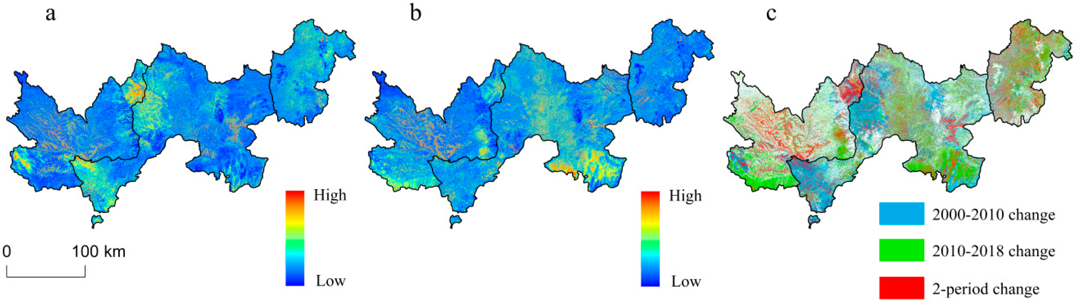
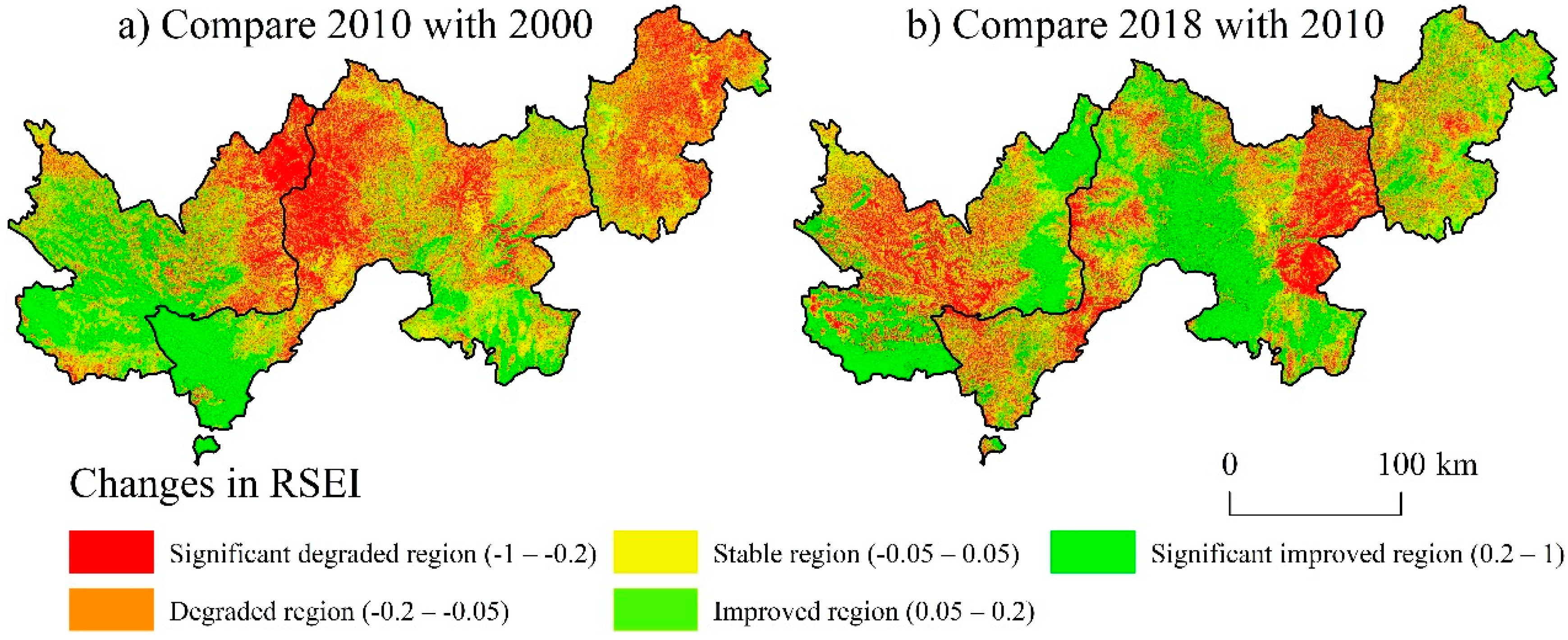
3.2. Spatiotemporal Changes in RSEI Based on the Change Vector Analysis (CVA) Method

The CVA method was used to analyze the spatiotemporal changes in RSEI in the study area. Complete CVA magnitude maps of the study area are presented in Figure 4. The high values of $\Vert \Delta E\Vert$, shown in red, appear in the western parts of the Gansu and Shaanxi tablelands from 2000–2010, and in the eastern part of Gansu tableland and southern part of Shaanxi tableland from 2010–2018. The Shanxi tableland has low $\Vert \Delta E\Vert$ values throughout the study period.

The suitable segmentation threshold for the change magnitude map was calculated using the Otsu method (Figure 4c). Changes from 2000–2010, 2010–2018, and both periods are represented by blue, green, and red pixels, respectively. In the Gansu tableland, blue pixels are mainly distributed in the southwest, and green pixels are mainly distributed in the south. The red pixels are mainly distributed in the northeast of this region, which indicated that the ecological environment there is relatively fragile. In the Shaanxi tableland, blue pixels are mainly distributed in the west and green pixels are mainly distributed in the central and southern parts of this region. Only a few red pixels are observed in the eastern part of this region. In the Shanxi tableland, there are relatively few areas with blue pixels, while there are green and red pixels over the entire area. In addition, the ecological environments of the northeastern Gansu tableland, southern Shaanxi tableland, and the entirety of the Shanxi tableland are fragile, with the RSEI of these regions presenting significant variation during the study period.

3.3. Spatial Distribution of the Different Grade of RSEI Variation

To investigate the variation in the RSEI between 2000 and 2018, we designated five labels to classify different regions of our study area: Significantly degraded, degraded, stable, improved, and significantly improved regions. The overall RSEI scale went from −1 to 2, determined by the differences in RSEI between 2010 and 2000 and between 2018 and 2010; each label corresponded to a certain interval in the scale (

Table 3. Spatial variation statistics table of RSEI in the study area.

Level	Interval	Gansu Tableland/%		Shaanxi Tableland/%		Shanxi Tableland/%
		2010–2000	2018–2010	2018–2000	2010–2000	2010–2000	2010–2000
Significant degraded region	−1–−0.2	17.65	20.75	21.02	21.85	26.69	11.92
Degraded region	−0.2–−0.05	20.95	16.46	21.78	18.53	37,44	21.72
Stable region	−0.05–0.05	19.02	17.39	21.77	16.85	20.77	24.6
Improved region	0.05–0.2	18.13	18.12	18.74	18.16	11.23	25.46
Significant improved region	0.2–1	24.25	27.28	16.70	24.61	3.86	16.3

). Figure 5 shows the spatial distribution of different grades in RSEI variations from 2000–2010 and 2010–2018. It can be seen that in the Gansu tableland, the overall area of significantly degraded and degraded regions decreased by 1.39% from 2000–2018. In addition, stable regions decreased by 1.63% while the overall area of significantly improved and improved regions increased by 3.02%, resulting in a global improvement in ecological quality. For the Shaanxi tableland, overall degraded regions decreased by 2.42%, stable regions decreased by 4.92%, and overall improved regions increased by 7.33% during the period 2000–2018. There were relatively larger variations in the Shanxi tableland: The area of degraded regions decreased by 30.49%, the area of stable regions was increased by 3.83%, and the area of overall improved regions increased by 26.67%.

The ecologically degraded areas of the Gansu tableland were mainly distributed in the southern parts of the Guchengchuan, Jiulonghe, Puhe, and Daxi rivers’ basins in the first ten years of the study. Ecologically stable areas were well spread throughout the tableland, while the ecological improvement areas were mainly distributed around the Weihe river. From 2010 to 2018, a large number of ecologically degraded areas appeared near the Puhe and Honghe rivers’ basins, while large ecological improvement areas appeared near the Daxi and the Guchengchuan rivers’ basins (Figure 5). Spatially, ecologically stable areas were often distributed around ecologically degraded regions.

In the Shaanxi tableland, only the areas around the Weihe and the Baishui rivers’ basins encountered some improvement, while most of the other areas experienced different levels of degradation from 2000 to 2010. Stable conditions were only observed for the areas in between the Sanshui river and the northern part of the Shajiachuan river’s basin. However, in the following eight years, except for some ecological degradation in contiguous regions around the Weihe, Sanshui, and the Ju rivers’ basins and on the eastern side of the Shaanxi tableland, most of the remaining areas in the Shaanxi tableland experienced some ecological improvement. This can be attributed to the execution of the positive measures discussed above, as well as to the efforts put into the restoration of vegetation.

As for the Shanxi tableland, almost the whole area went through ecological degradation from 2000 to 2010, with the exception of ecologically stable areas scattered around the Qinshui river’s basin, and some rare improvements only distributed in the northeast corner of the tableland. During the period from 2010 to 2018, ecological quality increased significantly in the whole tableland, but the areas around the Zhouchuan and the E rivers’ basins experienced further degradation, while the areas around the Qinshui river’s basin remained unchanged.

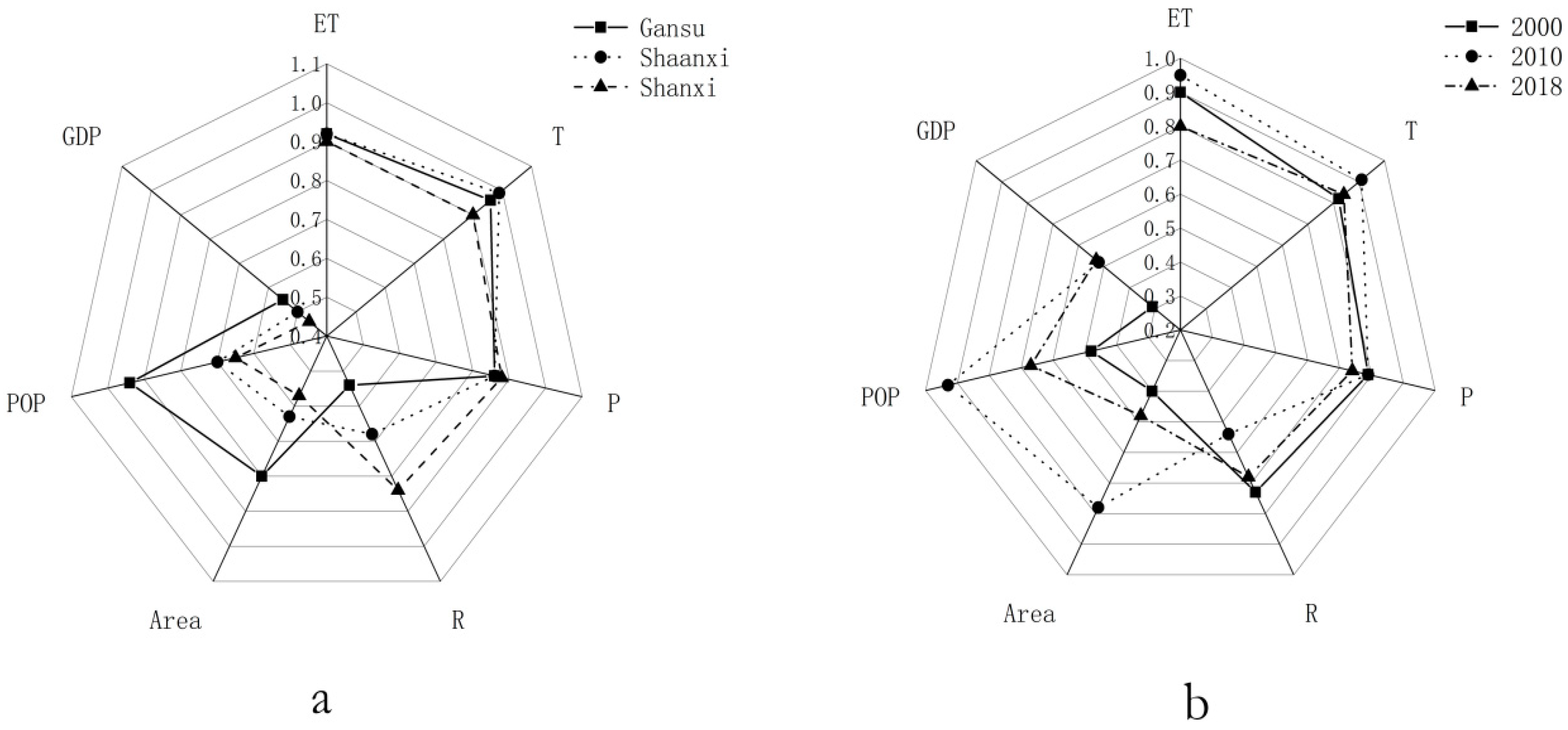
3.4. Contributing Factors for the Regional RSEI

For a long time, the pattern of severe droughts, soil erosion, sparse vegetation, population increases, low-efficiency economic models, and farmer poverty have been recognized as significant for the ecological security of the entire CLP [2]. Regional ecosystems consist of many factors, such as population, the economy, and the natural environment. There is also information uncertainty and incompleteness in these areas. A regional ecosystem is a gray system; in this, a model with a small data sample can be used to find a law for the system using sequence generation. Gray relation analysis can judge whether a connection is tight according to the similarity degree of sequence-curve geometry [48,49]. To determine which contributing factors had the main impact on the regional RSEI, the GRA analysis was carried out on some control factors that we considered of major importance: T, ET₀, R, P, GDP, AREA, and Pop.

Figure 6, which is based on the GRA results, shows the gray relational coefficient between different parameters and the RSEI. In the Gansu tableland, the ranking of the gray relational coefficients for the RSEI from 2000 to 2018 is T (0.96) > ET₀ (0.94) > POP (0.92) > P (0.86) > AREA (0.80) > GDP (0.55) > R (0.54). Natural parameters, including T, ET₀, and P, have a strong influence on the RSEI variations. The parameters POP (0.92) and Area (0.80) have a higher gray relational coefficient for the RSEI than other economic parameters, indicating that the rapidly increasing population and urban expansion contributed to the deterioration of the ecological environment of the study area. In the Shaanxi tableland, the ranking of the gray relational coefficient for the RSEI from 2000 to 2018 is T (0.99) > ET₀ (0.92) > P (0.81) > POP (0.70) > R (0.68) > AREA (0.63) > GDP (0.50). The RSEI variation of the Gansu tableland during the three periods showed strong association with the natural parameters apart from rainfall erosion. However, economic factors have not had a significant influence on the variation in the regional ecological environment in the Shaanxi tableland. As for the Shanxi tableland, the ranking of the gray relational coefficient between different parameters and the RSEI is T (0.90) > ET₀ (0.89) > P (0.88) > R (0.84)> POP (0.65) > AREA (0.57) > GDP (0.46). As with the Shaaxi tableland, the variation of RSEI is mainly controlled by natural factors, while the economic parameters have no obvious association with the variation in RSEI. In addition, the variation in rainfall erosion should be given more attention, as it has a significant influence on the variation of regional RSEI.

From a timewise perspective, the high gray relational coefficients for the RSEI in 2000 were ET₀ (gray relational coefficient of 0.90), T (0.8), and P (0.80). In this period, the regional ecological environment was mainly controlled by natural factors, such as temperature, evaporation, and precipitation; the interference of human activity had little influence on the regional ecological environment. In 2010, the ranking of the gray relational coefficient for the RSEI among the three tableland regions was ET₀ (0.95) > POP (0.93)> T (0.91) > P (0.79) > AREA (0.78) > R (0.54) > GDP (0.52). Population appeared to play an important role in the variation in RSEI during this period. Higher gray relational coefficients between population and RSEI indicated that the widespread human activity caused by the increasing regional population threatened the regional ecological environment in 2010. In 2018, the ranking of the gray relational coefficient for the RSEI among the three tableland regions is T (0.84) > ET₀ (0.80) > P (0.74) > POP (0.68) > R (0.48) > AREA (0.48) > GDP (0.53). The variation in the regional RSEI was only sensitive to variations in T and ET₀, which are both natural factors. The ecological environment of the tableland region of the CLP was particularly sensitive to variations in natural controlling factors, particularly temperature, potential evapotranspiration, and precipitation. The rapid increase in the regional population and human activity played an important role in varying the regional RSEI.

4. Conclusions

By analyzing and comparing the RSEI values, we can conclude that the eco-environmental quality improved in the Gansu tableland, remained stable in the Shaanxi tableland, and deteriorated in the Shanxi tableland between 2000 and 2018. We arrived at this conclusion because, from the beginning to the end of the study, there was a steady increase in the average RSEI value for Gansu, from 0.43 to 0.47; in the Shaanxi tableland, the average RSEI initially decreased from 0.45 (2000) to 0.43 (2010), and then increased to 0.45 (2018); while for Shanxi, the RSEI showed an initial decrease from 0.54 (2000) to 0.44 (2010), and then settled at 0.46 (2018).

The regions with poor or fair quality eco-environments were mainly concentrated in the Heihe, Daxi, Honghe, Puhe, Weihe, northern Sichuan, and E river basins. While human activity had a strongly negative impact on the ecological environment, the regions with moderate ecological conditions were always near those with poor conditions, which, in turn, are the poorer areas. It was not uncommon for poor areas to be subject to greater deterioration. The ecological conditions were good or excellent in the southern part of the E river. The ecological environments of the northeastern region of the Gansu tableland, the southern region of the Shaaxi tableland, and the entirety of the Shanxi tableland are fragile; the RSEI of these regions presented significant variation during the study period. More attention should be paid to the ecological security of the tableland region of the CLP. Natural factors, such as temperature, potential evapotranspiration, and precipitation, had the greatest influence on the overall ecological quality. The rapid increase in regional population and human activity played an important role in variation of the regional RSEI.

References

1. Li, S.; Liang, W.; Fu, B.J.; Lv, Y.H.; Fu, S.Y.; Wang, S.; Su, H.M. Vegetation changes in recent large-scale ecological restoration projects and subsequent impact on water resources in china’s loess plateau. Sci. Total Environ. 2016, 569–570, 1032–1039. [Google Scholar] [CrossRef]
2. Fu, B.J.; Wang, S.; Liu, Y.; Liu, J.B.; Liang, W.; Miao, C.Y. Hydrogeomorphic ecosystem responses to natural and anthropogenic changes in the loess plateau of china. Annu. Rev. Earth Planet. Sci. 2017, 45, 223–243. [Google Scholar] [CrossRef]
3. Wang, J.; Zhuo, J. Quantitative evaluation of soil erosion in returning farmland to forest area of loess plateau in north Shaanxi based on RS and GIS. Bull. Soil Water Conserv. 2015, 35, 220–223. [Google Scholar]
4. Groom, G.; Mücher, C.A.; Ihse, M.; Wrbka, T. Remote sensing in landscape ecology: Experiences and perspectives in a European context. Landsc. Ecol. 2006, 21, 391–408. [Google Scholar] [CrossRef]
5. Ochoa-Gaona, S.; Kampichler, C.; de Jong, B.H.J.; Hernández, S.; Geissen, V.; Huerta, E. A multi-criterion index for the evaluation of local tropical forest conditions in Mexico. For. Ecol. Manag. 2010, 260, 618–627. [Google Scholar] [CrossRef]
6. Sullivan, C.A.; Skeffington, M.S.; Gormally, M.J.; Finn, J.A. The ecological status of grasslands on lowland farmlands in western Ireland and implications for grassland classification and nature value assessment. Biol. Conserv. 2010, 143, 1529–1539. [Google Scholar] [CrossRef]
7. Gupta, K.; Kumar, P.; Pathan, S.K.; Sharma, K.P. Urban neighborhood green index—A measure of green spaces in urban areas. Landsc. Urban Plan. 2012, 105, 325–335. [Google Scholar] [CrossRef]
8. Xu, H.Q.; Ding, F.; Wen, X. Urban expansion and heat island dynamics in the quanzhou region, china. IEEE J. Sel. Top. Appl. Earth Obs. Remote Sens. 2009, 2, 74–79. [Google Scholar] [CrossRef]
9. Xu, H.Q.; Wang, Y.F.; Guan, H.D.; Shi, T.T.; Hu, X.S. Detecting Ecological Changes with a Remote Sensing Based Ecological Index (RSEI) Produced Time Series and Change Vector Analysis. Remote Sens. 2019, 11, 2345. [Google Scholar] [CrossRef] [Green Version]
10. Ivits, E.; Cherlet, M.; Mehl, W.; Sommer, S. Estimating the ecological status and change of riparian zones in Andalusia assessed by multi-temporal AVHHR datasets. Ecol. Indic. 2009, 9, 422–431. [Google Scholar] [CrossRef]
11. Caccamo, G.; Chisholm, L.A.; Bradstock, R.A.; Puotinen, M.L. Assessing the sensitivity of MODIS to monitor drought in high biomass ecosystems. Remote Sens. Environ. 2011, 115, 2626–2639. [Google Scholar] [CrossRef]
12. Willis, K.S. Remote sensing change detection for ecological monitoring in United States protected areas. Biol. Conserv. 2015, 182, 233–242. [Google Scholar] [CrossRef]
13. De Araujo Barbosa, C.C.; Atkinson, P.M.; Dearing, J.A. Remote sensing of ecosystem services: A systematic review. Ecol. Indic. 2015, 52, 430–443. [Google Scholar] [CrossRef]
14. Rouse, J.W.; Haas, R.H.; Schell, J.A.; Deering, D.W. Monitoring vegetation systems in the Great Plains with ERTS. NASA Spec. Publ. 1973, 351, 309–317. [Google Scholar]
15. Coutts, A.M.; Harris, R.J.; Phan, T.; Livesley, S.J.; Williams, N.S.G.; Tapper, N.J. Thermal infrared remote sensing of urban heat: Hotspots, vegetation, and an assessment of techniques for use in urban planning. Remote Sens. Environ. 2016, 186, 637–651. [Google Scholar] [CrossRef]
16. Estoque, R.C.; Murayama, Y. Monitoring surface urban heat island formation in a tropical mountain city using Landsat data (1987–2015). ISPRS J. Photogramm. Remote Sens. 2017, 133, 18–29. [Google Scholar] [CrossRef]
17. Malbéteau, Y.; Merlin, O.; Gascoin, S.; Gastellu, J.P.; Mattar, C.; Olivera-Guerra, L.; Khabba, S.; Jarlan, L. Normalizing land surface temperature data for elevation and illumination effects in mountainous areas: A case study using aster data over a steep-sided valley in morocco. Remote Sens. Environ. 2017, 189, 25–39. [Google Scholar] [CrossRef] [Green Version]
18. Tiner, R.W. Remotely-sensed indicators for monitoring the general condition of “natural habitat” in watersheds: An application for Delaware’s Nanticoke River watershed. Ecol. Indic. 2004, 4, 227–243. [Google Scholar] [CrossRef]
19. Mildrexler, D.J.; Zhao, M.S.; Running, S.W. Testing a MODIS global disturbance index across North America. Remote Sens. Environ. 2009, 113, 2103–2117. [Google Scholar] [CrossRef]
20. Healey, S.P.; Cohen, W.B.; Yang, Z.Q.; Krankina, O.N. Comparison of tasseled cap-based Landsat data structures for use in forest disturbance detection. Remote Sens. Environ. 2005, 97, 301–310. [Google Scholar] [CrossRef]
21. Rhee, J.; Im, J.; Carbone, G.J. Monitoring agricultural drought for arid and humid regions using multi-sensor remote sensing data. Remote Sens. Environ. 2010, 114, 2875–2887. [Google Scholar] [CrossRef]
22. Xu, H.Q. A remote sensing urban ecological index and its application. Acta Ecol. Sin. 2013, 24, 7853–7862. [Google Scholar]
23. Zhang, C.; Xu, H.Q.; Zhang, H.; Tang, F.; Lin, Z.L. Fractional vegetation cover change and its ecological effect assessment in a typical reddish soil region of southeastern china: Changting county, Fujian province. J. Nat. Resour. 2015, 6, 917–928. [Google Scholar]
24. Yang, F.H.; Song, J.J.; Zhao, Y.R.; Zhao, J.L.; Niu, C. Dynamic monitoring of ecological environment in black soil erosion area of northeast China based on remote sensing. Res. Environ. Sci. 2018, 9, 1580–1587. [Google Scholar]
25. Zhang, X.D.; Liu, X.N.; Zhao, Z.P.; Ma, Y.Y.; Yang, Y. Dynamic monitoring of ecology and environment in the agro-pastral ecotone based on remote sensing: A case of Yanchi county in Ningxia hui autonomous region. Arid Land Geogr. 2017, 5, 1070–1078. [Google Scholar]
26. Fu, B.J.; Liu, Y.; Lv, Y.H.; He, C.S.; Zeng, Y.; Wu, B.F. Assessing the soil erosion control service of ecosystems change in the Loess Plateau of China. Ecol. Complex. 2011, 8, 284–293. [Google Scholar] [CrossRef]
27. Lü, Y.H.; Fu, B.J.; Feng, X.M.; Zeng, Y.; Liu, Y.; Chang, R.Y.; Sun, G.; Wu, B.F. A policy-driven largescale ecological restoration: Quantifying ecosystem services changes in the loess plateau of china. PLoS ONE 2012, 7, e31782. [Google Scholar]
28. Su, C.H.; Fu, B.J. Evolution of ecosystem services in the Chinese loess plateau under climatic and land use changes. Glob. Planet. Chang. 2013, 101, 119–128. [Google Scholar] [CrossRef]
29. Fu, B.J.; Zhang, L.W.; Xu, Z.H.; Zhao, Y.; Wei, Y.P.; Skinner, D. Ecosystem services in changing land use. J. Soils Sediments 2015, 15, 833–843. [Google Scholar] [CrossRef]
30. Sun, C.J.; Chen, W.; Chen, Y.; Cai, Z. Stable isotopes of atmospheric precipitation and its environmental drivers in the Eastern Chinese Loess Plateau, China. J. Hydrol. 2019, 581, 124404. [Google Scholar] [CrossRef]
31. Lü, Y.H.; Zhang, L.W.; Feng, X.M.; Zeng, Y.; Fu, B.J.; Yao, X.L.; Wu, B.F. Recent ecological transitions in china: Greening, browning, and influential factors. Sci. Rep. 2015, 5, 8732. [Google Scholar] [CrossRef] [PubMed]
32. Liang, W.; Bai, D.; Wang, F.Y.; Fu, B.J.; Yan, J.P.; Wang, S.; Yang, Y.T.; Long, D.; Feng, M.Q. Quantifying the impacts of climate change and ecological restoration on streamflow changes based on a Budyko hydrological model in china’s loess plateau. Water Resour. Res. 2015, 51, 6500–6519. [Google Scholar] [CrossRef]
33. Cao, Z.; Li, Y.R.; Liu, Y.H.; Chen, Y.F.; Wang, Y.S. When and where did the Loess Plateau turn “green”? Analysis of the tendency and breakpoints of the normalized difference vegetation index. Land Degrad. Dev. 2017, 29, 162–175. [Google Scholar] [CrossRef]
34. Sun, C.J.; Zheng, Z.J.; Chen, W.; Wang, Y.Y. Spatial and Temporal Variations of Potential Evapotranspiration in the Loess Plateau of China during 1960–2017. Sustainability 2020, 12, 354. [Google Scholar] [CrossRef] [Green Version]
35. Kilic, A.; Allen, R.; Trezza, R.; Ratcliffe, I.; Kamble, B.; Robison, C.; Ozturk, D. Sensitivity of evapotranspiration retrievals from the METRIC processing algorithm to improved radiometric resolution of Landsat 8 thermal data and to calibration bias in Landsat 7 and 8 surface temperature. Remote Sens. Environ. 2016, 185, 198–209. [Google Scholar] [CrossRef] [Green Version]
36. Xu, H.Q.; Huang, S.L.; Zhang, T.J. Built-up land mapping capabilities of the ASTER and Landsat ETM+ sensors in coastal areas of southeastern China. Adv. Space Res. 2013, 52, 1437–1449. [Google Scholar] [CrossRef]
37. Hu, X.S.; Xu, H.Q. A new remote sensing index for assessing the spatial heterogeneity in urban ecological quality: A case from Fuzhou city, china. Ecol. Indic. 2018, 89, 11–21. [Google Scholar] [CrossRef]
38. Yue, H.; Liu, Y.; Li, Y.; Lu, Y. Eco-Environmental Quality Assessment in China’s 35 Major Cities Based on Remote Sensing Ecological Index. IEEE Access 2019, 7, 51295–51311. [Google Scholar] [CrossRef]
39. Crist, E.P. A TM Tasseled Cap equivalent transformation for reflectance factor data. Remote Sens. Environ. 1985, 17, 301–306. [Google Scholar] [CrossRef]
40. Baig, M.H.A.; Zhang, L.F.; Shuai, T.; Tong, Q.X. Derivation of a tasseled cap transformation based on Landsat 8 at-satellite reflectance. Remote Sens. Lett. 2014, 5, 423–431. [Google Scholar] [CrossRef]
41. Rikimaru, A.; Roy, P.S.; Miyatake, S. Tropical forest cover density mapping. Trop. Ecol. 2002, 43, 39–47. [Google Scholar]
42. Xu, H.Q. A new index-based built-up index (IBI) and its eco-environmental significance. Remote Sens. Technol. Appl. 2017, 3, 301–308. [Google Scholar]
43. Chander, G.; Markham, B.L.; Helder, D.L. Summary of current radiometric calibration coefficients for Landsat MSS, TM, ETM+, and EO-1 ALI sensors. Remote Sens. Environ. 2009, 113, 893–903. [Google Scholar] [CrossRef]
44. Sobrino, J.A.; Jiménez-Muñoz, J.C.; Paolini, L. Land surface temperature retrieval from LANDSAT TM 5. Remote Sens. Environ. 2004, 90, 434–440. [Google Scholar] [CrossRef]
45. Li, P. Research on Information Extraction Method of Vegetation Coverage Change Based on CVA; Capital Normal University: Beijing, China, 2011. [Google Scholar]
46. Dewi, R.S.; Bijker, W.; Stein, A. Change vector analysis to monitor the changes in fuzzy shorelines. Remote Sens. 2017, 9, 147. [Google Scholar] [CrossRef] [Green Version]
47. Xu, H.Q.; Wang, M.Y.; Shi, T.T.; Guan, H.D.; Fang, C.Y.; Lin, Z.L. Prediction of ecological effects of potential population and impervious surface increases using a remote sensing based ecological index (RSEI). Ecol. Indic. 2018, 93, 730–740. [Google Scholar] [CrossRef]
48. Huang, J.T.; Liao, Y.S. Optimization of machining parameters of Wire-EDM based on Grey relational and statistical analyses. Int. J. Prod. Res. 2003, 41, 1707–1720. [Google Scholar] [CrossRef]
49. Huang, Z.B.; Xu, M.; Chen, W.; Lin, X.J.; Cao, C.X.; Ramesh, P.S. Postseismic restoration of the ecological environment in the Wenchuan region using satellite data. Sustainability 2018, 10, 3990. [Google Scholar] [CrossRef] [Green Version]
Figure 1. Location of the study area of the Chinese Loess Plateau (CLP).
Sustainability 12 03489 g001
Figure 2. The variation in the different grades of remote sensing ecological index (RSEI) values during the study period.
Sustainability 12 03489 g002
Figure 3. Spatial distribution of different RSEI quality grades in (a) 2000, (b) 2010, and (c) 2018.
Sustainability 12 03489 g003
Figure 4. Change magnitude map of RSEI in (a) 2000–2010 and (b) 2010–2018; (c) change intensity map of RSEI.
Sustainability 12 03489 g004
Figure 5. Spatial distribution of RSEI different change grades in (a) 2000–2010 and (b) 2010–2018.
Sustainability 12 03489 g005
Figure 6. The wind rose encompassing each controlling factor of the RSEI in the CLP for (a) three tableland regions, (b) three periods.
Sustainability 12 03489 g006