Article

U.S. State-level Projections of the Spatial Distribution of Population Consistent with Shared Socioeconomic Pathways

by
Hamidreza Zoraghein
1,* and
Brian C. O’Neill
2
1
Office of Social & Behavioral Science Research, Population Council, New York, NY 10017, USA
2
Pardee Center for International Futures and Josef Korbel School of International Studies, University of Denver, Denver, CO 80208, USA
*
Author to whom correspondence should be addressed.
Sustainability 2020, 12(8), 3374; https://doi.org/10.3390/su12083374
Submission received: 23 March 2020 / Revised: 8 April 2020 / Accepted: 9 April 2020 / Published: 21 April 2020

Abstract

:
Spatial population distribution is an important determinant of both drivers of regional environmental change and exposure and vulnerability to it. Spatial projections of population must account for changes in aggregate population, urbanization, and spatial patterns of development, while accounting for uncertainty in each. While an increasing number of projections exist, those carried out at relatively high resolution that account for subnational heterogeneity and can be tailored to represent alternative scenarios of future development are rare. We draw on state-level population projections for the US and a gravity-style spatial downscaling model to design and produce new spatial projections for the U.S. at 1 km resolution consistent with a subset of the Shared Socioeconomic Pathways (SSPs), scenarios of societal change widely used in integrated analyses of global and regional change. We find that the projections successfully capture intended alternative development patterns described in the SSPs, from sprawl to concentrated development and mixed outcomes. Our projected spatial patterns differ more strongly across scenarios than in existing projections, capturing a wider range of the relevant uncertainty introduced by the distinct scenarios. These projections provide an improved basis for integrated environmental analysis that considers uncertainty in demographic outcomes.

1. Introduction

Projections of the spatial distribution of population are consequential for integrated human-environment analysis. Population and its spatial distribution are drivers of land-use/land-cover change [1,2] and greenhouse gas emissions [3], both with significant impacts on the climate, biodiversity, and air quality. Temporal changes of population also play a significant role in determining urbanization regimes and the extent to which human’s presence in the form of built-up areas is spatially distributed [4]. Projections of the spatial distribution of population also help identify those that are likely to be most affected by climate change and other environmental stress, which can inform resource allocation, adaptation, and mitigation policies in relation to environmental hazards. For example, such projections have been used to find that the increasing likelihood of storm surge and coastal flooding ensuing from sea level rise [5] may impact the considerable proportion of the world population that is already living close to coastal areas [6,7]. Moreover, the combination of global warming and changes in the spatial distribution of the population driven by urbanization will lead to more people being exposed to severe heatwaves [8,9]. Climate change can also influence the distribution of land area capable of supporting vector-borne diseases [10,11], which can lead to greater human exposure [12]. In addition to such projections that shed light on the population exposure to the detrimental effects of climate change, studies have started to augment them with supplementary demographic attributes such as income distribution and age structure to address challenges in vulnerability differentiation of the population [13,14].
The use of alternative scenarios for future conditions of society and the environment is a common approach in human-environment analysis to address uncertainty. Each scenario represents a plausible and unique future formed by a collection of determining inputs, and the set of scenarios as a whole addresses uncertainty by incorporating all these distinct possibilities. The production of alternative spatial population projections, as elements of broader societal scenarios, has been an important component of this collective perspective on uncertainty. For the U.S. region, a previous study downscaled the U.S. population at the Census division level to 1/8° resolution grids consistent with the A2 and B2 socioeconomic scenarios from the Special Report on Emissions Scenarios (SRES) [15]. Researchers in [16] used U.S. Census-based projections to derive county-level population aggregates and downscaled them to grids in 2030 and 2050. Researchers in [17] generated a series of global population projection grids by downscaling country level population projections under the Shared Socioeconomic Pathways (SSPs) [18] for the 2010–2100 period. Other US projections consistent with the SSPs have been produced at the county level [19,20,21] but not downscaled to the grid cell level.
SSPs are widely adopted in the human-environment analysis community as a set of qualitative narratives describing different societal development pathways with distinct implications in the societies’ capacity for adaption to or mitigation of climate change effects [18]. The SSP narratives have been complemented by quantitative projections of several socioeconomic attributes reflecting distinct patterns of national-level population growth and educational composition [22], urbanization level [23] and economic growth [24]. Combined with climate models, SSP projections offer a widely-used, comprehensive framework to assess the mutual effects between climate change and society [25,26,27]. They also play a crucial role in enhancing the effectiveness of adaptation and preparedness programs in relation to environmental hazards by identifying the most vulnerable segments of the society.
The SSPs have been defined to formulate challenges that societal conditions would present to adaptation to climate change and mitigation of emissions. However, they are not subtle enough in their original form to formulate future socioeconomic conditions at local or regional scales. To foster incorporating the SSP framework across specific domains and geographic scales, their global definitions need to be extended and encompass local or regional subtleties that are eclipsed in the global version. Previous studies have already highlighted the importance of this topic and developed and applied extended SSPs to specific applications such as population dynamics in coastal areas and determinants of human vulnerability in Europe [26,28].
This study follows an ongoing research endeavor whose objective is to provide different SSP-based demographic attributes specific to each U.S. state, by which their associated uncertainty is considered. It generates projections of spatial population distribution for each state for the 2020–2100 period by downscaling their population aggregates to 1 km resolution grids. The downscaling employs a gravity-based model tailored to each state, which is documented in [29] and is based on previous work for generating scenario-based population distributions [15,17,30]. State-level population aggregates draw on [31], who extend national-level SSP2, SSP3, and SSP5 assumptions of fertility, mortality, and migration to each state and project population by age and sex for each state as a whole accordingly using a demographic cohort component model (Appendix A.1).
In the following section, we describe the SSPs and explain how we implement their corresponding assumptions about total population, urbanization, and spatial development patterns. We then describe our methodology for producing spatial projections for the U.S. by summarizing the gravity model structure and detailing the approach we use to modify its parameters to produce development patterns consistent with the SSPs. We then present our spatial population projection results according to the SSPs and discuss their distinguishing features. We conclude this paper by summarizing the lessons learned through the analysis and potential areas of improvement.

2. SSPs and Their Demographic Assumptions

The SSPs consist of five alternative socioeconomic pathways that societies could follow in the future, in terms of their demographics, human development, economy, lifestyle, policies, technology, and environment and natural resources, which have significant implications for their climate-related adaptation and mitigation capacities. SSP1(Sustainability) describes a development path that emphasizes environmental protection, reduced inequality, and significant investment in education and health. SSP2 (Middle of the Road) envisions a world whose various aspects of socioeconomic development resemble historical trends. SSP3 (Regional Rivalry) leads to a world with a dominant presence of nationalism and security concerns, resulting in regionalization, slow economic growth, and low investment in human capital and education. SSP4 (Inequality) is similar to SSP3 in terms of neglecting sustained investment in human development but differs in that it depicts a world with a widening gap between the majority of the society and a small, well-educated, and internationally connected elite class, within countries as well as across them. SSP5 (Fossil-fueled Development) envisions a world with substantial focus on globalization, international competitive markets, and rapid economic growth that produce high levels of human development. However, it relies on fossil fuels and lacks sustainable environmental protection policies exercised in SSP1.
Three factors determine spatial population projections in each state, namely its population aggregate, urbanization level, and spatial distribution pattern. We, therefore, employ assumptions on these determinants conforming to three of the SSPs (SSP2, SSP3, and SSP5) to incorporate uncertainty and inform our spatial population projections. We choose these SSPs based on the availability of state-level population and urbanization projections for each of them, as well as the fact that they span the full range of national population size across the SSPs and have a diversity of assumptions about spatial development patterns. For population, we use the quantitative results of recent state-level projections from [31], who use a demographic cohort component model to generate state-level population aggregates based on assumptions on future fertility, mortality, domestic, and international migration in each state that are consistent with the SSPs (Appendix A.1). In summary, at the national level the three SSPs lead to a range of U.S. population from ~246 to 650 million by 2100 (Table A1 and Figure A1), a range that is somewhat lower than the range in the original SSP population projections (~451 million) [22] due primarily to updated base year data showing lower current levels of fertility and migration ([31] and Appendix A.1).
SSP2 leads to moderate population changes reflecting historical fertility, mortality, and migration trends. Due to the high income levels, investments in human capital, and relatively open borders that SSP5 envisions, this scenario is associated with the highest fertility and migration and lowest mortality projections, resulting in the highest population growth. Conversely, SSP3 is a scenario of low income growth, relatively low investment in human capital, and limited international flows, which translate to low fertility and migration, resulting in the slowest population growth and even population decline in some states over the course of the projection period. The projections assume that domestic migration between states retain the currently observed regional pattern, but the overall scale of that migration is highest in SSP5 and lowest in SSP3. The projections lead to substantial heterogeneity in population growth across states, ranging for example from substantial decline in some states and SSPs (e.g., the Northeast in SSP3) to substantial growth in others (e.g., Utah and Texas in SSP5), covering uncertainty in different pathways that the population of states might take.
For urbanization, we use SSP-based projections of the share of urban population by state from a model based on observed trends in urbanization patterns at the national and sub-national level [32], summarized and illustrated in Appendix A.2 (Table A2 and Figure A2). The rapid economic growth according to SSP5 produces large urban employment opportunities and high migration rates. Therefore, urbanization grows rapidly in this scenario, and large numbers of people move to cities. In contrast, the economic uncertainty associated with SSP3 manifests itself in a paucity of employment opportunities in urban areas and low migration rates. These two features contribute to slow urbanization in this scenario. SSP2, as a moderate scenario that is situated in the middle of the spectrum, envisions moderate urbanization.
Regarding spatial development patterns, we adopt the qualitative assumptions in the SSP narratives to support our modeling choices [17]. SSP5 leads to rapid economic and urbanization growth. However, sustainable planning in this scenario is not prioritized as opposed to SSP1. Thus, urban planning cannot keep up with the large influx of population, leading to a sprawling spatial distribution of population extending from cities. On the other hand, urban areas fail to attract population as strongly in SSP3. Combined with the lack of planning in this scenario, this results in a spatial distribution of population which is neither consolidated nor sprawling but rather a mixed pattern. SSP2 conforms to the historical spatial distribution of population and depending on the area, it can follow consolidation, sprawl or mixed.

3. Methodology

Our projection model downscales state-level rural/urban SSP-based population aggregates to 1-km resolution grids to produce total population grids from 2020 to 2100 at 10-year intervals, with a 2010 base year. We use a gravity-based population downscaling model described elsewhere [15,17,29] to generate population grids according to the three SSPs. In addition to the input data, the model relies on two parameters that govern the importance to the projected distribution of population of current population centers and distance. These two parameters can be used to reflect the assumed features of the spatial distribution patterns for each scenario. In the following sections, we first briefly describe the model and then explain how we derived parameter values for each scenario. The input data and outputs of the model can be found at [33], and the code for generating the results is available from [34].

3.1. Gravity-based Population Downscaling Model

The gravity-based model downscales state-level population in the next projection year to its constituent grid cells by allocating the aggregate population change between the current and projection years to each cell proportional to its suitability value (or to the inverse of its suitability value in case of population decline). Its foundational mathematical equation is as follows:
v i = l i j = 1 n P j α × e β d i j
In Equation 1, vi is the suitability value estimated for the focal cell, i, li is the mask value modifying the suitability of the focal cell, depending on its topographic and land-use/land-cover characteristics, Pj is the total population of the neighboring cell, j, and dij is the distance between the focal cell and its neighboring cell. The summation over j is performed for n cells contained in the neighborhood within 100 km of the focal cell, representing a distance estimate over which existing amenities are influential in attracting population in the U.S. [35]. The α and β parameters govern the importance of existing surrounding population concentrations (within the neighborhood defined by n) and their accessibility (a function of distance) in determining the suitability value, respectively. The suitability calculation is carried out separately for the urban and rural population within each cell (a distinction not represented here), with separate parameter values for each although the population Pj in Equation 1 represents the total population in both cases.
Figure 1 demonstrates how the model works. For each state, the population grid in the first year, aggregate population in the second year, as well as α and β parameters are specific to each scenario (except when the first year is the base year 2010, when all scenarios share the same starting distribution). Notably, the process is stepwise, i.e., creating population grids in 2020 requires them in 2010 and so on. Therefore, the downscaling process under each scenario starts at 2010 and finishes in 2100. We projected urban and rural population separately in each step and then added their grids to create total population grids. We utilized state-level urban/rural population grids at 1-km resolution in 2010 generated from its urban/rural census blocks and a spatial mask created by state-level topographic and land-use/land-cover layers [29].
The model has been calibrated and evaluated against historical data for the 1990–2000 and 2000–2100 periods and shown to perform reasonably well against recent experience [29]. It performs better in simulating observed changes in the distribution of urban than rural populations, and estimated urban population parameters are more stable over time. It is well suited for the production of alternative future scenarios, including those that diverge from historical patterns of development, due to its ability to control spatial patterns in a relatively straightforward manner with two parameters and to interpret those parameters clearly in terms of the patterns of development they produce.

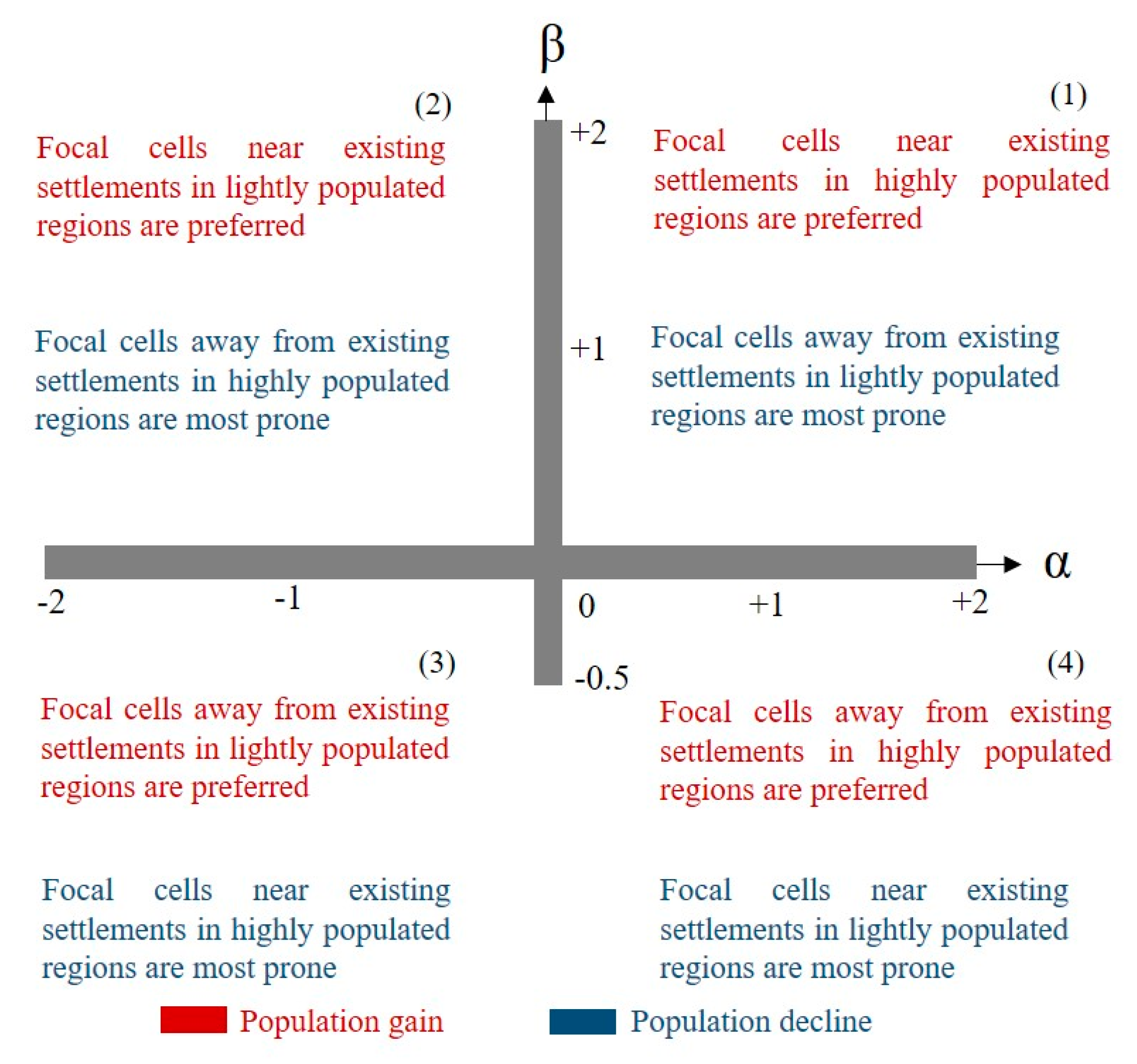
3.2. Modification of Parameters According to SSPs

The modification of the α and β parameters to conform to SSP assumptions about spatial development is based on the semantic framework in [29], which interprets different parts of the two-dimensional parameter space in terms of their qualitative implications for spatial development patterns (Figure 2).
The α parameter indicates the degree to which the population size of surrounding cells translates into the suitability of a focal cell. A positive value indicates that the larger the population that is located within the 100 km neighborhood, the more suitable the focal cell is (while a negative value of alpha would imply a less suitable focal cell). The β parameter reflects the significance of distance to surrounding cells on the suitability of a focal cell. Within 100 km, β determines how distance modifies the effect on suitability. Because the exponent in Equation 1 is the negative of β, the higher the positive value of the parameter, the greater the deterrent effect of distance. In contrast, negative values of the parameter imply a lower friction of distance. When β is 0, it means distance does not matter, and each cell contributes to the suitability of the focal cell proportional to its population raised to α. Figure 2 summarizes these interpretations.
Table A3 in Appendix A.3 includes estimated state-level rural and urban parameters [29]. We used the semantic framework along with historical parameters to determine parameters for SSP2, SSP3, and SSP5. Employing the semantic framework facilitates mapping parameters to the spatial change pattern prescribed by each SSP, while considering historical parameters ensures that new parameters will not diverge too quickly from their current values.
Because the SSP2 scenario is intended to resemble historical trends, we used parameter values for each state in this scenario as estimated from historical data for the 2000–2010 decade and kept them constant over time. The process for estimating these parameters is shown in Figure A3. These historical values imply consolidated urban population patterns since the parameters for nearly all states fall in the first quadrant of the parameter space (Figure A4). For most states, rural population parameters also fall in this quadrant (Figure A5), although some fall within the second and fourth quadrants, favoring low density growth near small towns (and consolidation-oriented pattern in case of population decline) and sprawl pattern, respectively.
SSP3 envisions a mixed spatial change pattern, in which populous agglomerations are not attractive due to economic stagnation, population distribution planning is not prevalent and investment in infrastructure is limited. All these factors guided our decision to change current parameters over time toward the second quadrant in Figure 2, which represents a development pattern favoring low density population growth (or disfavoring population sprawl around large cities in case of population decline). This pattern is distinct from sprawl in that growth does not occur near high population centers (cities) but rather near smaller towns. We linearly changed rural parameters for each state to begin at their recent values and reach alpha, beta values of (−2, 2) in the year 2050, as a representative point of the second quadrant. The choice of the year 2050 for the time at which scenario-specific parameter values are reached was made in order to avoid parameter changes that represented sudden changes in patterns (which are not indicated by the SSP storylines, which emphasize more gradual change), while still occurring early enough in the century to produce distinguishable population outcomes across the different SSPs.
However, there was no instance of historical urban parameters in the second quadrant except for Michigan, where special circumstances (the depopulation of Detroit) occurred. Therefore, we instead used the top left location in the first quadrant (0, 2) (Figure A4), into which all other recent historical experience has fallen, as the target values for urban parameters reached by all states in 2050. This choice therefore adopts the parameter values closest to the low-density development pattern of the SSP narrative that is still informed by historical experience (Figure A4).
SSP5’s assumption of a sprawling spatial population change pattern with attractive populous areas is implemented by assuming that parameters move toward the fourth quadrant, representing a sprawling pattern of development. For rural parameters, we chose (1, −0.5) because it represents the pattern associated with the fourth quadrant and does not diverge too substantially from historical rural parameters in that quadrant (Figure A5). However, because there was no historical precedent for an urban parameter in the fourth quadrant, we chose the bottom right location of the first quadrant (2, 0), where nearly all historical values fall, as the values that are closest to the sprawling pattern of development while still being informed by historical experience (Figure A4).

4. Results and Discussion

In this section we present spatial population projection results based on SSP2, SSP3, and SSP5 that are consistent with state-level population totals for those scenarios [31]. We analyze population grids for the contiguous U.S. and for selected states and evaluate the differences in spatial population distribution across scenarios. We also compare the resulting grids with those from the global spatial projections developed previously [17].

4.1. SSP Projections

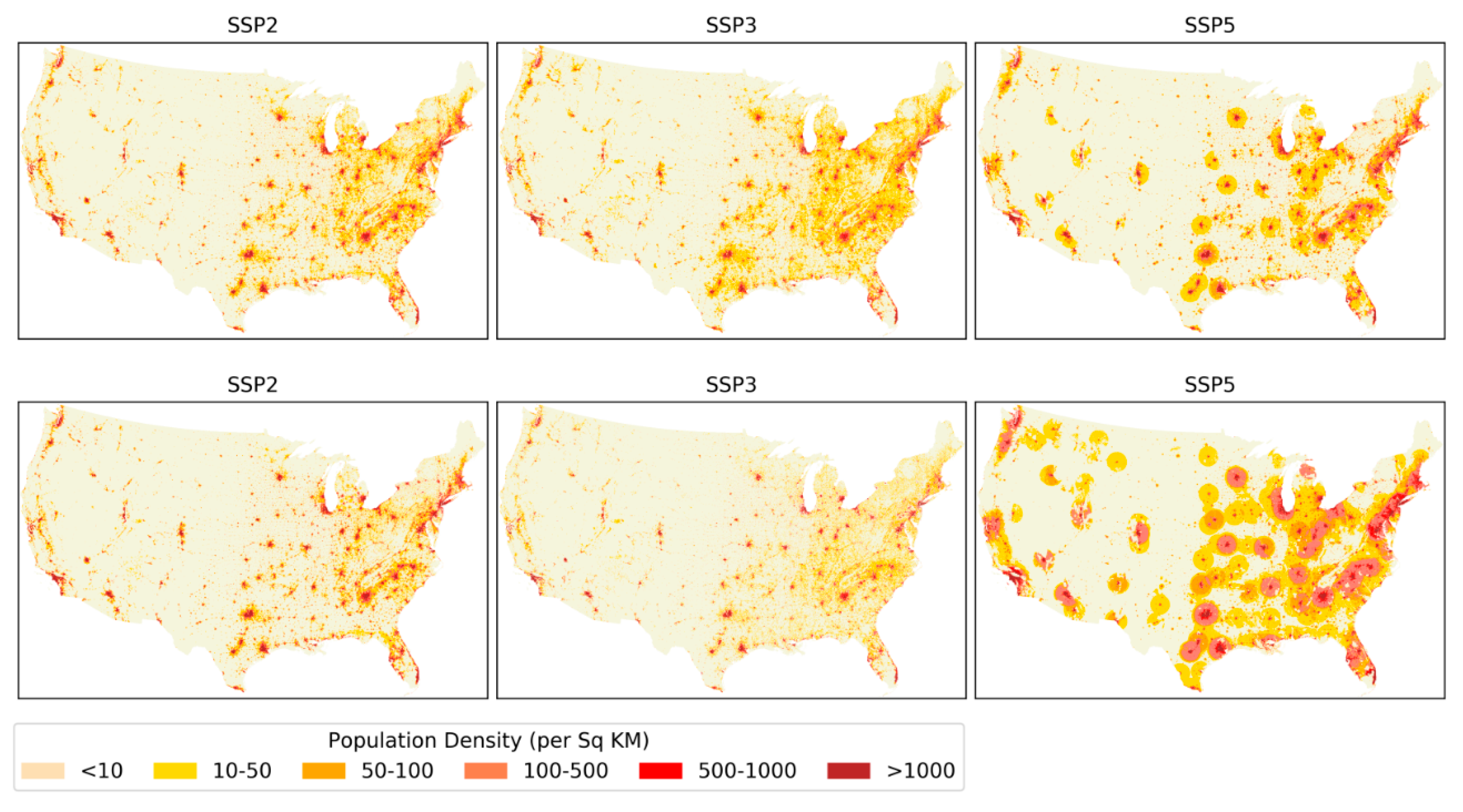
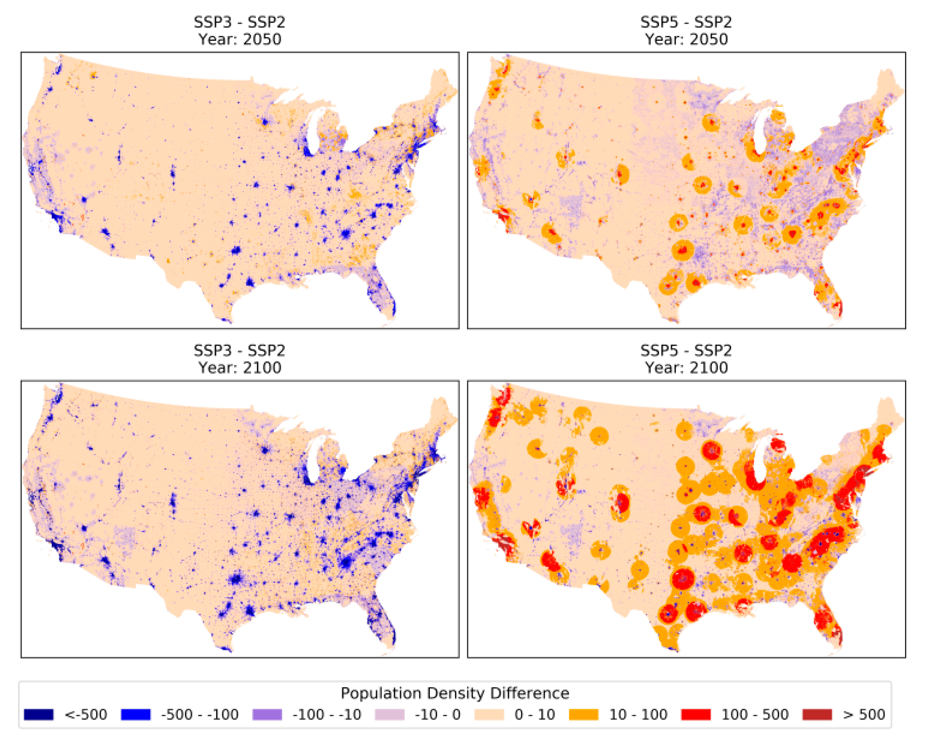
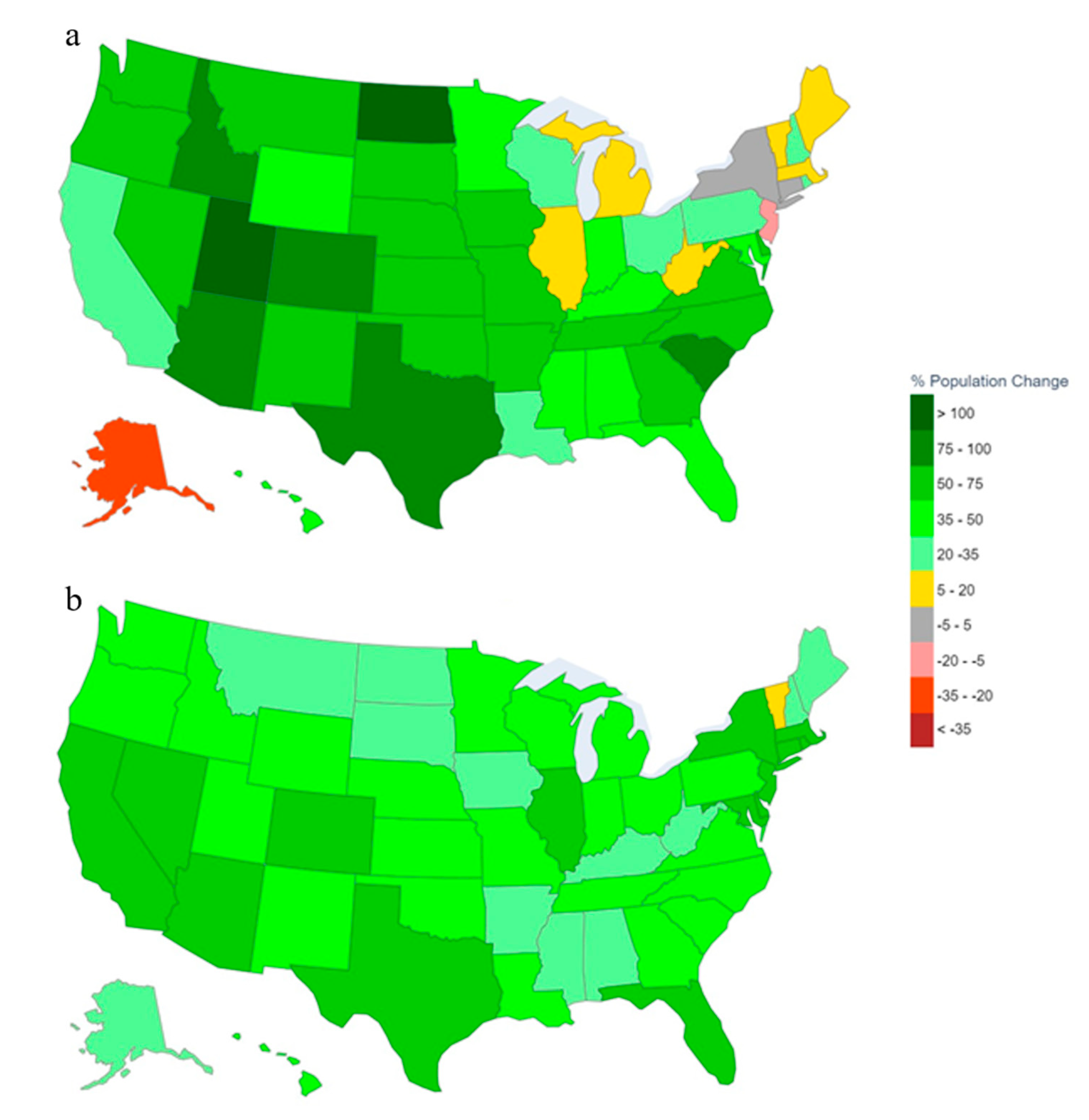
4.1.1. National SSP Projections

Figure 3 shows population projections for the contiguous U.S. consistent with SSP2, SSP3, and SSP5 in 2050 and 2100. Results are consistent with expectations based on the SSP narrative descriptions of spatial development patterns and our implementation of them in model parameter values. The discrepancy in results stems from the inherent uncertainty about population aggregates in states, their urbanization levels and spatial development patterns mandated by each scenario. For example, Figure 3 demonstrates the dominant urbanization and sprawl pattern in SSP5, especially in 2100, resulting from rapid population growth, the importance of current populous centers (high α) and the insignificance of distance to population location within their 100 km surroundings (low β). The relatively circular development patterns around most large cities result from the gravity model’s approach of estimating suitability values from population within a commonly defined neighborhood, combined with a lack of features around these cities that would lead to spatial mask values discouraging development in particular directions. For places surrounded with physical obstacles and topographic constraints, such as coastal cities in the Northeast, the Bay Area, Seattle, Los Angeles, Phoenix, or Denver, the expansive urban development is asymmetric, excluding areas that are deemed uninhabitable by the spatial mask layer. SSP3 shows dispersed distributions with less population in urban areas, a result of low population growth (even decline in some states) and lack of attractiveness of such areas to absorb population, combined with parameter values that favor growth in areas of low population density.
The SSP2 pattern is in between the others in terms of population in or near urban areas given its moderate population growth and urbanization, with these areas clearly less populated than SSP5 while they host more people than SSP3. In addition, SSP2 exhibits a more concentrated development pattern due to parameter values consistent with recent historical experience, which tends toward concentrated development and allows less dispersal.
To clarify the contrast across SSPs, Figure 4 shows maps of population differences between SSP3 or 5 on the one hand and SSP2 on the other, in 2050 and 2100. Differences are due both to differences in aggregate state populations between scenarios as well as to differences in spatial distribution patterns; in the next section, we isolate the effect of spatial patterns for individual states.
Results confirm that between SSP5 and SSP2, growing positive population differences around urban agglomerations point to the strong sprawl effect in SSP5 contrasted with the concentrated development pattern in SSP2. Negative population differences in rural areas reflect the stronger urbanization trends in SSP5 that lead to more significant movements away from such areas as compared to SSP2. Comparing SSP3 with SSP2 confirms that urban areas have substantially smaller populations in SSP3. In 2050, there are patches of positive population difference in rural areas, which are no longer evident in 2100 due to the overall population decline at the national level according to SSP3.

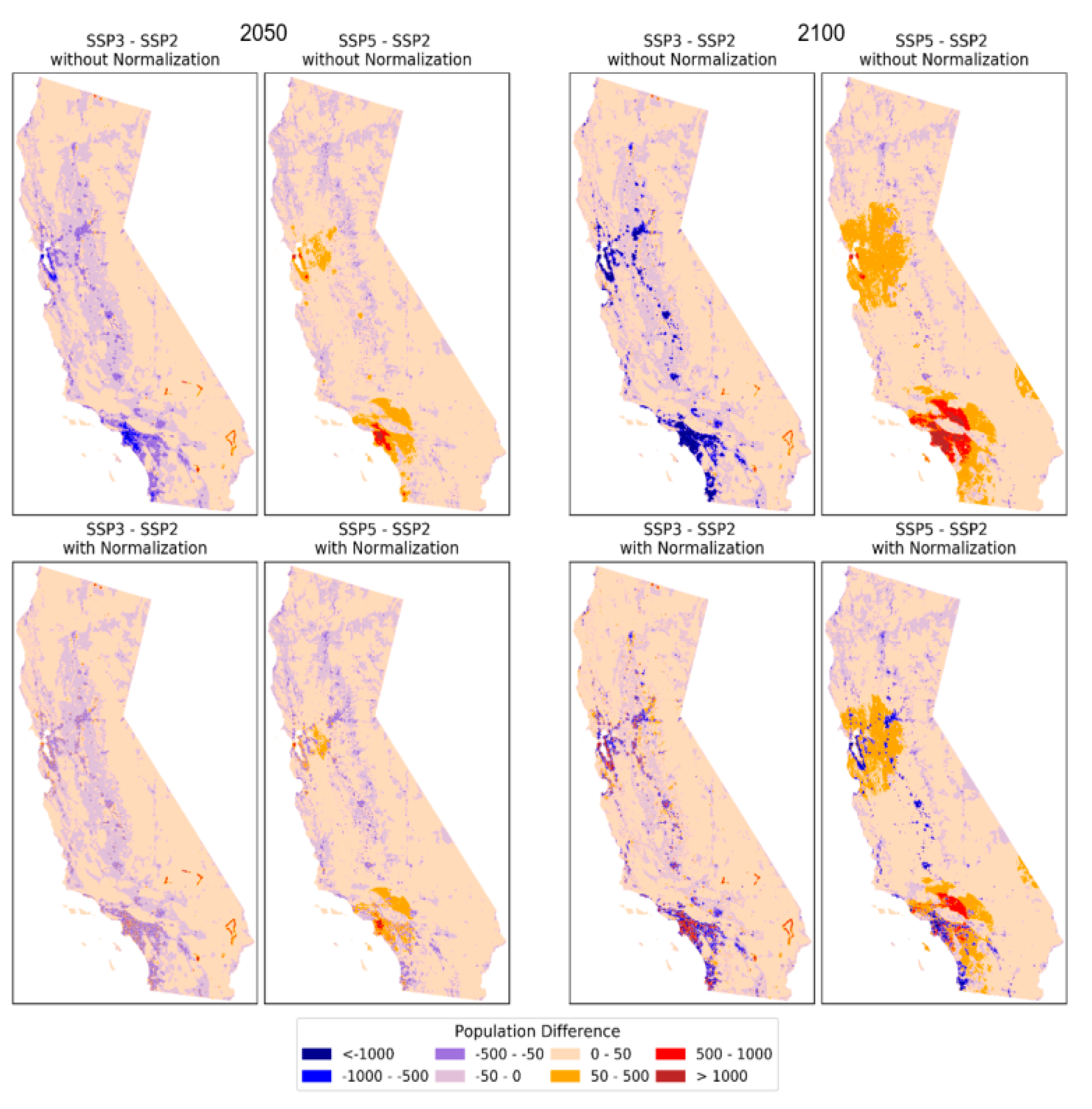
4.1.2. State level SSP Projections

In addition to the national level results, this section describes population projection results at the state level. We chose California as an example for this section as a large state with a diversity of development patterns. Appendix A.4 presents similar results (Figure A6 and Figure A7) and interpretations for New York as an example of a state with more frequent population decline in its projections. According to state-level population projection results in [31], the total population of California increases under SSP2 (moderately) and SSP5 (rapidly), whereas in SSP3 it first increases gradually until 2050 and then declines over the 2050–2100 period such that its population in 2100 (~27 million) is projected to be lower than its current population (~37 million).
Figure 5 compares SSP3- and SSP5-based population grids of California with its SSP2-based grids in 2050 and 2100. To control for the effect of differences in total state population across SSPs, we also normalized SSP3- and SSP5-based population grids to match the SSP2 total state population by adjusting the population of all cells by the same proportion. This allows us to assess the specific effect of differences in spatial model parameters across scenarios on the resulting distributions of population.
By 2050, SSP3 leads to lower population in urban areas compared to SSP2 while SSP5 results in higher population in these areas, also spread over a larger suburban area. The same pattern, but to a lesser extent, exists after normalization, indicating that both differences in spatial parameters and total population contribute in a similar way to overall differences in outcomes.
By 2100, the raw (non-normalized) differences across scenarios are larger and of the same nature. SSP3 results in substantially lower population in urban areas and their surroundings (and in fact declining population over time in an absolute sense as well), whereas SSP5 results in much higher populations in these areas. However, the normalized results indicate some differences in the contribution of the spatial development pattern per se to these overall outcomes. In SSP3, the lower population outcomes (compared to SSP2) are distributed away from urban centers, consistent with this scenario’s development pattern in which population loss preferentially occurs in suburban areas (Figure 2). This pattern is more evident in 2100 than it is in 2050 because spatial model parameters only reach their scenario-specific values in 2050, and so by 2100 the parameters have had 50 years to fully affect the spatial distribution outcomes. Normalization of the SSP5 projection, on the other hand, demonstrates that positive population differences under this scenario are larger in the surroundings of urban agglomerations and are actually negative in the city centers. This reflects the full expression of the differences between SSP5 as a sprawling scenario and SSP2 that has concentrated development.

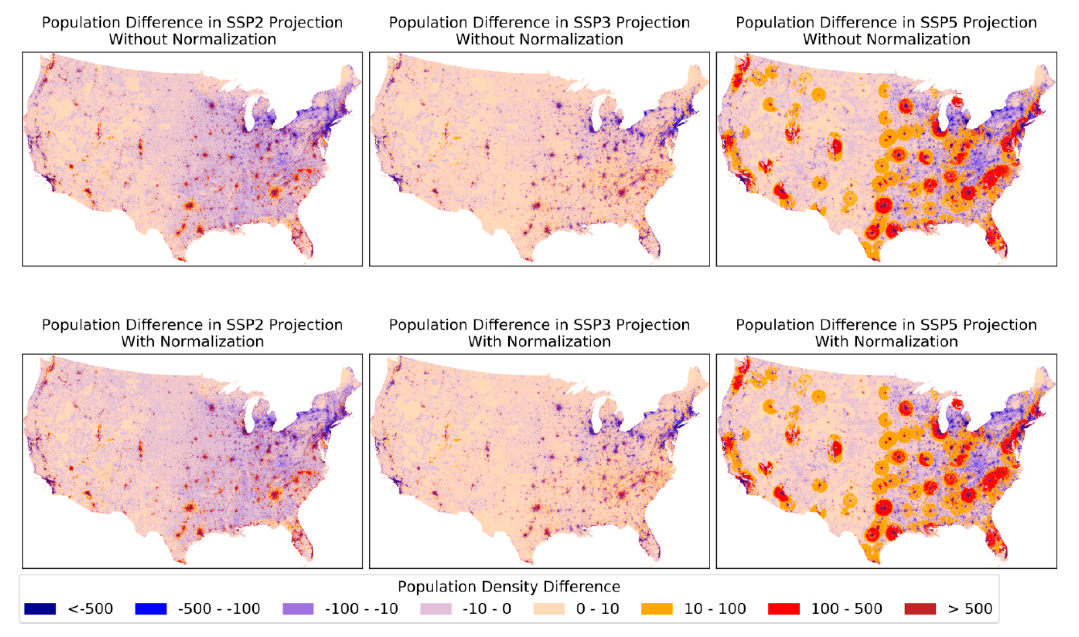
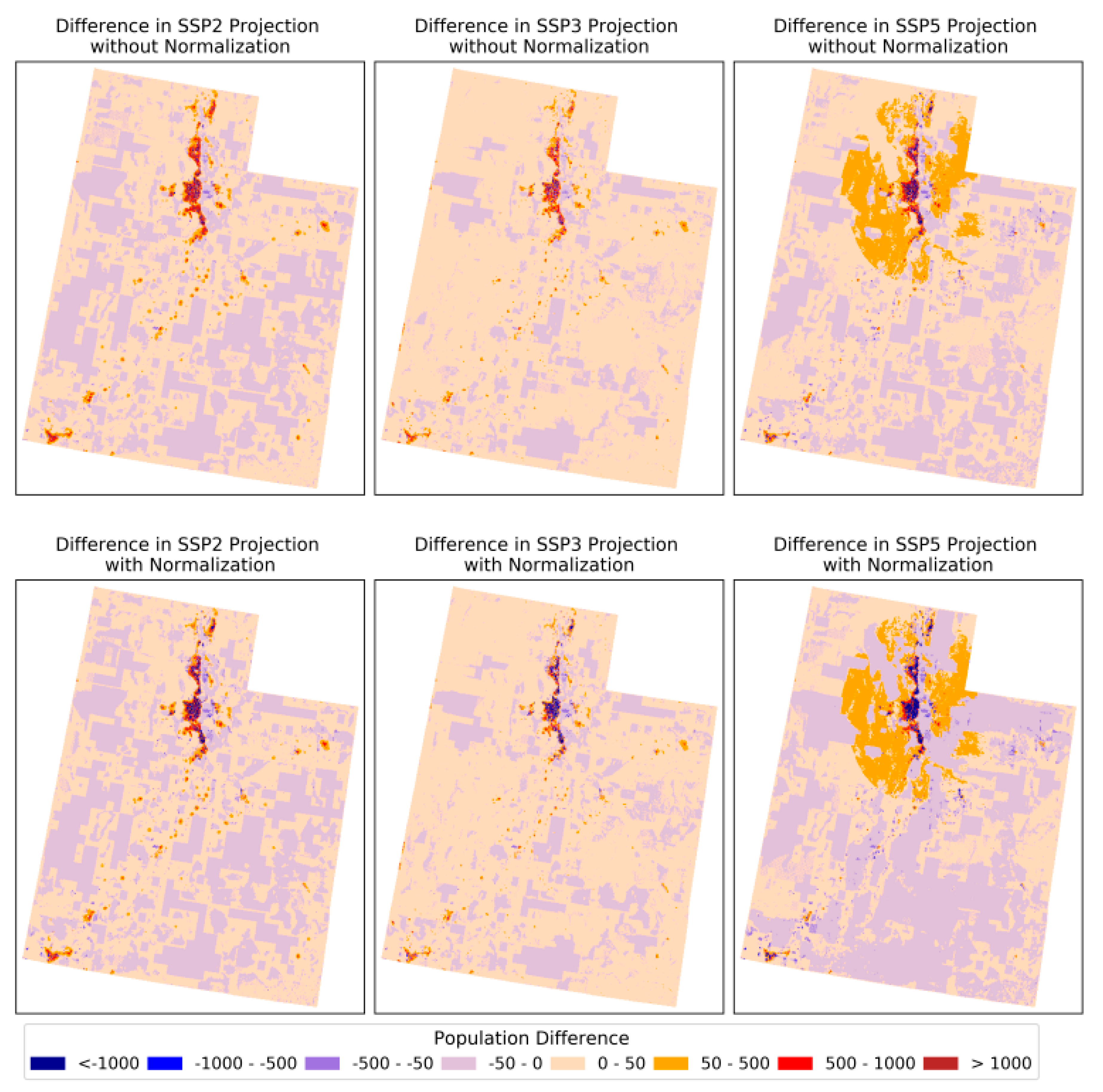
4.2. Comparison to the Current National Model

This section compares population grids from the global spatial population projection model described in [17] to the grids projected here. The primary differences between these two models are summarized as follows:
  • The global model downscales SSP-based national population aggregates of each country [22] to its constituent grid cells whereas the state-level model downscales each U.S. state’s population [31] to its grid cells. The most important difference between these projections is that the state-level model produces redistribution of the population across states through differences in fertility, mortality, and (especially) migration at the state level while the global model does not (Appendix A.5 and Figure A8 in Appendix A as well as [36]).
  • The global model uses a single set of spatial parameters that is estimated from data for the whole country, and are applied to the entire country while the state-level model estimates and applies parameters specific to each state (except for after 2050 in SSPs 3 and 5 when all states have the same parameters).
  • The initial spatial resolution of the global model is 1/8° that has been downscaled to 1 km resolution grids [37]. The resolution of the state-level model is 1 km, and therefore we used the 1 km version of the global model for the comparison.
  • The global model uses datasets that are globally available while the state-level model leverages datasets that are specific to the U.S.
  • The base year of the global model is 2000, and it generates projections from 2010 to 2100 at 10-year intervals while the base year of the state-level model is 2010 and it creates population projection grids from 2020 to 2100 at the same interval.
Figure 6 compares population projection grids consistent with SSP2, SSP3, and SSP5 from the state-level model in 2100 with the corresponding grids from the global model. Because the global model is based on higher fertility and international migration assumptions, it leads to higher national population totals in 2100 compared to the state-level model (Figure A1 in Appendix A). Therefore, we also normalized grids derived from the global model to ensure their aggregates are equal to those from the state-level model. Figure 6 shows that differences after normalization are too subtle to notice at the national scale, and there are differences between the projections that are robust to whether normalization is applied or not. First, the SSP2 grid from the state-level model leads to a more concentrated population distribution pattern, consistent with our parameters that are estimated separately for each state and reflect recent experience of consolidation, especially for urban populations. Population allocated to remote rural areas is lower in the state-level model while positive population differences are observed in urban areas. Second, the SSP5 grid from the state-level model leads to a much stronger sprawl pattern around urban centers compared to the global model, depicted by its dominantly positive differences in such areas. Third, overall differences in the population of some regions are evident across all SSPs, especially SSP2 and SSP3. In the state-level population projection model, areas such as New England and California (and to some extent the Great Lakes region) experience substantial negative net domestic migration and low fertility, resulting in lower regional populations compared to the global model, which cannot capture well these regional re-distributions of population (Figure A8 in Appendix A).
To explore the regional differentiation in the state-level model further, we also present projected population differences for two sample states, one with smaller population in the state-level model because of its lower projected fertility and higher domestic out-migration (Massachusetts) and the other with higher population as a result of its higher projected fertility and domestic in-migration (Utah). For the global model values, the corresponding grids were upscaled to the state boundaries (Table A4 in Appendix A.6).
Figure 7 shows that the difference grids for Massachusetts are dominantly negative partly as a result of the lower projected population in 2100 in the state-level model to begin the downscaling process with. However, there are also substantial differences between the normalized projections. In SSP2 and especially SSP3, the state-level model produces generally lower population in suburban and rural areas, while in SSP5 suburban populations are larger and populations nearer to city centers are smaller. This suggests that the state-specific parameters, and the choices of parameter values for the different SSPs produce a wider range of spatial patterns in the state-level model compared to the global model.
In contrast, Figure 8 shows that the state-level model produces an overall higher population than the global model; the normalized differences show that spatial patterns differ as well. Across all SSPs, the state-level model allocates more population to areas around populated centers, and less to areas in or near the center. SSP5 also shows a much more pronounced sprawl pattern in the state-level model.

5. Conclusions

In this paper, we downscaled U.S. state level population aggregates to their constituent grid cells. To demonstrate uncertainty in projections of the spatial distribution of population, we produced them based on three alternative scenarios, namely SSP2, SSP3, and SSP5, that are widely used in human-environment dynamics analysis. Each scenario envisions an alternative socioeconomic path that societies might follow with distinct implications for their capacity to respond to climate change. In addition to differences in population aggregates and urbanization levels that these scenarios entail, each leads to an alternative spatial pattern of population distribution. We used a semantic framework that interprets quantitative values of spatial population model parameters in qualitative terms to design spatial projections that are consistent with the narrative descriptions of intended development patterns in the SSPs.
We presented population projection grids consistent with the three SSPs at both national and state levels in 2050 and 2100. These grids depict spatial distributions of population that align with our expectation from each SSP. SSP5 leads to the most dominant population sprawl pattern, whereas SSP3 results in the most dispersed distribution with the lowest growth in populous urban areas. SSP2, as a moderate scenario, leads to distributions in the middle of the divide in terms of overall urbanization but that emphasizes concentrated growth. Comparing projections normalized for different total populations at the national and state levels showed that our SSP-based projections differences are driven to a substantial extent by differences in spatial patterns of development within states.
Finally, we compared our spatial population projections with the projections from a global model that downscaled national (as opposed to state-level) population totals [17]. The differences show that spatial patterns consistent with each SSP are more pronounced in the state-level model used in this paper, thereby providing a wider coverage of uncertainty. There are also disparities in outcomes for population across broad regions, due to the ability of the state-level model to account for migration between states and heterogeneity in other demographic rates. Population is generally smaller in our projections compared to the global model in New England and California, where regional fertility and domestic migration are projected to be low.
Global spatial projections such as those from [17] are valuable because they use a methodology and are based on data that can be applied consistently across all countries of the world. We believe that projections such as ours offer improved country-specific results because they can take advantage of more and higher resolution data for a specific country that may not be available elsewhere, draw on subnational aggregate projections (such as for states) that can capture demographic heterogeneity, and estimate parameters that vary across subnational units.
However, future work could improve on this projection and others like it. Regarding the spatial model itself, obtaining a longer time series of past spatial population data would allow for parameter estimation over a longer period, more consistent with the long-term projections to which the model is applied. Although parameters are estimated separately for states and urban and rural populations, further differentiation would likely improve model performance and its flexibility for projecting future patterns, including distinguishing spatial patterns around larger and smaller cities and towns, and differentiating within rural areas between very low density areas and rural areas that are closer to suburban developments. Regarding scenario definition, testing the robustness or projections of alternative but equally plausible specifications of parameter values consistent with qualitative storylines, including their changes over time, would be valuable.
Our future work will complete the SSP projections for SSP1 and SSP4 to generate a series of state-level population distributions consistent with all five SSPs. We also plan to incorporate age structure into our spatial projections [13]. These developments, combined with integration with alternative climate projections, will enable more effective analysis of questions about the exposure and vulnerability of the U.S. population to environmental hazards such as sea level rise and heat waves in the future.

Author Contributions

Conceptualization, H.Z. and B.C.O.; Data curation, H.Z.; Formal analysis, H.Z.; Funding acquisition, B.C.O.; Investigation, H.Z. and B.C.O.; Methodology, H.Z. and B.C.O.; Project administration, B.C.O.; Supervision, B.C.O.; Visualization, H.Z.; Writing—original draft, H.Z.; Writing—review & editing, B.C.O. All authors have read and agreed to the published version of the manuscript.

Acknowledgments

This research was supported by the U.S. Department of Energy, Office of Science, as part of research in Multi-Sector Dynamics, Earth and Environmental System Modeling Program.

Conflicts of Interest

The authors declare no conflict of interest. The funders had no role in the design of the study; in the collection, analyses, or interpretation of data; in the writing of the manuscript; or in the decision to publish the results.

Appendix A

This appendix contains additional text, tables, and figures on six topics:
  • State-level population projections
  • State-level urbanization projections
  • Estimated parameters of the population downscaling model
  • SSP projections for New York
  • Regional redistribution in state-level projections
  • Population summary of Massachusetts and Utah

Appendix A.1. State-Level Population Projections

The state-level population projection model is fully described in [31]; we provide a brief overview here. The study uses a demographic cohort component model to project the population of each state disaggregated by age and gender at 1-year intervals from 2010 to 2100. The model uses inputs from the 2010 U.S. Census, the American Community Survey (ACS) and the U.S. Centers for Disease Control (CDC) Wonder database to create historical records of fertility, mortality, domestic migration and international migration for each state. It then uses both historical records and SSP-based demographic projections for the U.S. derived from [22] to construct SSP-based projections of the aforementioned variables at the state level and eventually of the total population.
To make assumptions for each state on future changes in fertility, mortality, and international migration, their methodology assumes that the changes in these rates at the national level apply equally (in proportional terms) to all states. Given the heterogeneity in age structures and demographic rates across states, this application of uniform proportional changes in future rates will not result in uniform changes in growth rates or age structures across states, thereby introducing regional population variation across states according to their demographic profile. They produce state-level projections consistent with SSP2, SSP3 and SSP5. To make assumptions on changes in domestic migration, they assume that trends in domestic migration would be qualitatively similar to those in international migration; that is, in a scenario like SSP5 with high international migration, domestic migration would also be high. This extends the concept in SSP5 of a globalizing world with low barriers to people’s movement to the domestic level. The same concept is applied to the low migration SSP3 scenario.
The state-level total population projections when aggregated to the national level diverge from the original national level SSP projections by [22] (Figure A1) mainly because they are based on more recent data for current conditions with lower fertility and migration compared to the original SSP projections, and they make alternative assumptions about international migration beyond 2050 (relaxing the assumption in the original projections that international migration converges to zero in the long run). In addition, in the state-level projections, shifts in the composition of the population across states can change national growth rates as compared to a national model.
Figure A1. Population projections for the U.S. in SSP2 (solid line), SSP3 (dotted line), and SSP5 (dashed line) after aggregating state-level projections (blue) [31], compared to the original national level SSP projections (grey).
Sustainability 12 03374 g0a1
Table A1 presents state-level population projections consistent with SSP2, SSP3 and SSP5 in 2050 and 2100 as well as their values in 2010.
Table A1. State-level population projections consistent with SSP2, SSP3 and SSP5 (divided by 1000) [31].
State SSP2SSP3SSP5
2010205021002050210020502100
Alabama47805920698051213918694311,083
Alaska710488526422299495726
Arizona6249926611,2447967636010,88517,082
Arkansas2916378446073273259544707339
California37,23544,10346,73038,85227,36048,54068,917
Colorado50277522920864755187879013,976
Connecticut3574367036253243213340115360
Delaware89812681474108482414812204
D.C.6027538266474637761108
Florida18,80123,01026,00419,68414,10527,25640,716
Georgia968813,10915,45411,321870115,22223,847
Hawaii1360174820191492113219302855
Idaho1568237830182037172927684498
Illinois12,83013,33813,48411,781785414,36619,769
Indiana64257933898168975209886713,146
Iowa3046392447703427284044577057
Kansas2853387247703336275143957015
Kentucky43395450642547363661637410,116
Louisiana4533524959504574336459479248
Maine132813731433119780915992287
Maryland57747047786960874409797311,708
Massachusetts65487455781664884444827011,434
Michigan988410,29810,6969048634011,04315,114
Minnesota53046443731256484356716810,676
Mississippi2967351440223046226240136255
Missouri59897665915965935138881213,840
Montana98912661543109586815002424
Nebraska1826249731702170190528134544
Nevada2701377944203259247544066729
New Hampshire131615261630133195117202427
New Jersey87928313763773434460875710,824
New Mexico2059271032752335187130724829
New York19,37619,47818,69517,21010,95220,49226,174
North Carolina953513,48516,25911,510893515,96325,170
North Dakota6731047134591682011941944
Ohio11,53712,83414,02411,214812014,40421,145
Oklahoma3751495461054310348658439735
Oregon38315303637545543498635610,109
Pennsylvania12,70214,40315,50312,542888016,26723,213
Rhode Island105311991278104674613211846
South Carolina46256661824456874551801512,984
South Dakota8141057129592877512001924
Tennessee63468110959970065385953715,157
Texas25,14636,66545,33131,80025,93942,78170,405
Utah2764476564494140395753148870
Vermont6266426625643797241011
Virginia800110,85012,7049287704112,41218,859
Washington6725951311,5248161639511,17617,738
West Virginia1853186119961637112921653259
Wisconsin56876460688356794031722410,317
Wyoming5646968396064837951260

Appendix A.2. State-Level Urbanization Projections

The state-level urbanization projection model is fully documented elsewhere [32]; we provide a brief overview here. This state-level model tailors the global model described in [23] to the subnational level and projects urbanization under different scenarios for the 2010-2100 period. The model first constructs a database of historical records of the total population and urbanization levels (percent of the population defined as urban) of world countries, U.S. states, China provinces and India states. For each U.S. state, the model first identifies the current urbanization level and trend of that state, and then searches all historical records to find instances in which other regions had similar urbanization conditions. It finally categorizes those regions into “slow”, “central” and “fast” groups based on the urbanization growth rate they experienced after that point in time and uses them to construct three alternative projection pathways for the U.S. state being projected. As an example, if a U.S. state is currently 60% urban with an increasing urbanization level, the model finds all regions that at some point in the past were 60% urban and uses their subsequent urbanization trajectories to inform the projections for the U.S. state.
The model repeats this process in 2040, starting with projected urbanization conditions of U.S. states at that time, so that projections are carried out in two stages. This allows the model to project a total of nine alternative pathways of urbanization for each target region, characterized by its pace of urbanization in the near term (through 2040) and the longer term (beyond 2040), namely “slow-slow”, “slow-central”, “slow-fast”, “central-slow”, “central-central”, “central-fast”, “fast-slow”, “fast-central” and “fast-fast”. Figure A2 shows different urbanization projection pathways for Alabama.
The next step is to map the nine pathways to the different SSP scenarios. Because SSP3 and SSP5 envision slow and fast urbanization growth, respectively, and SSP2 points to a middle-of-the-road scenario, we assigned the “central-central”, “slow-slow”, and “fast-fast” projections to the SSP2, SSP3 and SSP5 scenarios, respectively. Table A2 presents state-level urbanization projections consistent with SSP2, SSP3 and SSP5 in 2050 and 2100 as well as their values in 2010.
Figure A2. Alternative urbanization projections for Alabama [32].
Sustainability 12 03374 g0a2
Table A2. State-level urbanization projections consistent with SSP2, SSP3 and SSP5 [32].
State SSP2SSP3SSP5
2010205021002050210020502100
Alabama59.074.986.361.065.087.495.7
Alaska66.079.789.267.770.988.696.1
Arizona89.694.497.989.087.797.799.7
Arkansas56.273.183.158.162.988.298.4
California95.097.098.590.887.999.099.6
Colorado86.292.996.286.686.897.199.0
Connecticut88.093.997.388.488.797.198.8
Delaware83.390.695.184.987.095.698.7
D.C.100.0100.0100.0100.0100.0100.0100.0
Florida91.295.098.889.486.998.399.8
Georgia75.185.591.778.181.594.399.1
Hawaii91.996.398.790.087.598.099.2
Idaho70.682.491.372.375.494.699.4
Illinois88.594.397.988.288.097.899.3
Indiana72.384.493.074.778.895.699.5
Iowa64.077.087.165.668.787.195.0
Kansas74.285.191.876.780.094.698.9
Kentucky58.474.785.860.364.087.998.0
Louisiana73.284.693.175.879.194.599.1
Maine38.760.276.039.843.478.192.7
Maryland87.293.397.287.187.197.498.9
Massachusetts92.096.498.989.686.798.699.8
Michigan74.685.792.077.882.194.598.7
Minnesota73.384.493.375.378.594.699.1
Mississippi49.468.082.351.058.083.996.2
Missouri70.483.291.171.474.495.299.6
Montana55.972.482.857.962.887.297.7
Nebraska73.184.293.075.578.694.699.4
Nevada94.297.299.390.786.898.999.7
New Hampshire60.374.986.762.265.687.795.7
New Jersey94.796.797.990.187.398.999.7
New Mexico77.487.393.079.983.694.799.1
New York87.993.797.288.489.297.098.7
North Carolina66.178.888.468.371.688.496.2
North Dakota59.975.186.662.165.987.796.2
Ohio77.987.693.281.185.294.699.2
Oklahoma66.279.889.268.071.488.896.3
Oregon81.089.394.783.185.096.099.0
Pennsylvania78.787.993.080.785.195.399.3
Rhode Island90.795.198.489.587.898.399.8
South Carolina66.378.988.368.672.188.596.1
South Dakota56.773.283.359.064.486.096.4
Tennessee66.479.589.168.071.489.196.6
Texas84.791.295.086.287.696.499.0
Utah90.694.798.290.288.697.399.0
Vermont38.960.276.039.641.879.294.0
Virginia75.586.091.878.181.794.499.4
Washington84.191.195.085.987.496.198.8
West Virginia48.766.281.450.157.083.796.0
Wisconsin70.282.491.171.775.294.799.4
Wyoming64.878.088.066.669.788.196.1

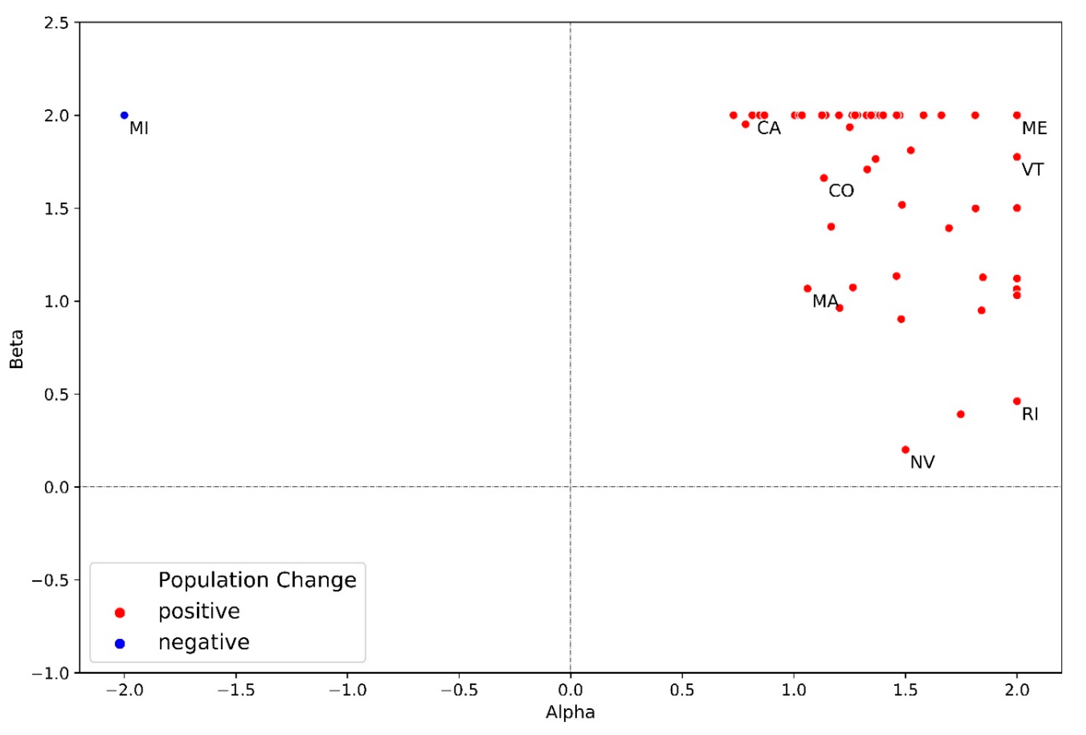
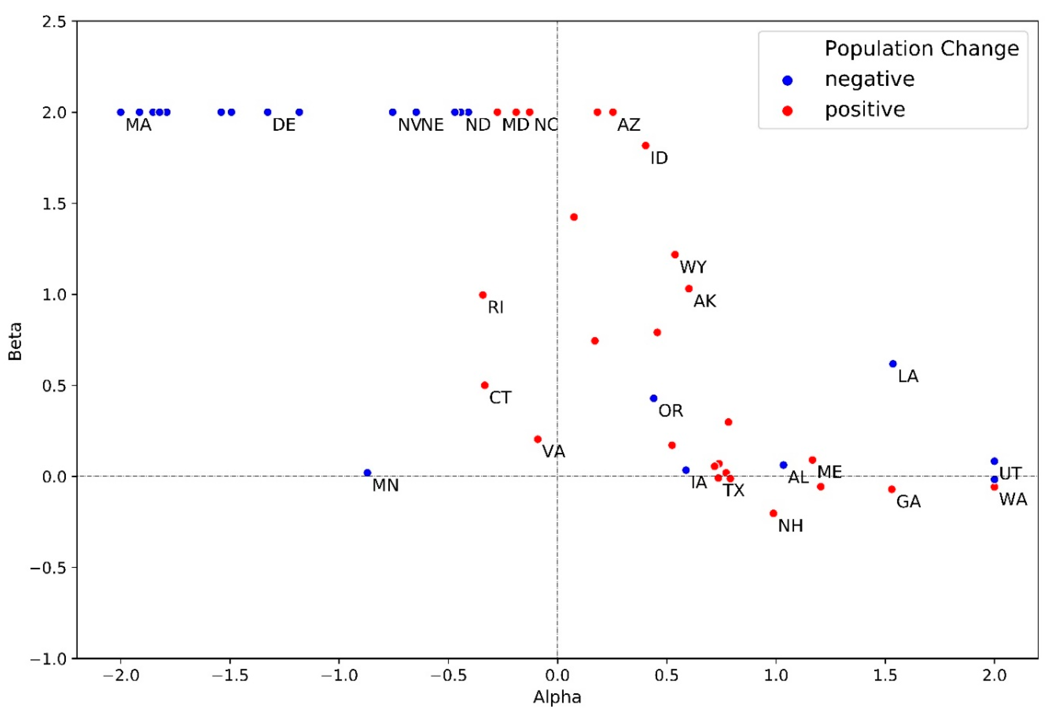
Appendix A.3. Estimated Parameters of The Population Downscaling Model

The calibration and validation component of the spatial downscaling model is fully documented in [29]; we summarize key features here and provide the estimated parameter values. The model is grounded in historical population grids in 2000 and 2010 and estimates urban and rural parameters for each state that minimize the difference between the projected population grids in 2010 and their corresponding census block-based grids. Figure A3 demonstrates the calibration process, leading to the parameters that are used in the spatial downscaling model in the base year of all SSPs and that are kept constant over time in SSP2. Figure A4 and Figure A5 plot the estimated urban and rural parameters, and Table A3 summarizes them for all states.
Figure A3. The calibration process of the gravity-based population downscaling model [29].
Sustainability 12 03374 g0a3
Figure A4. Scatterplot of state-level urban α and β parameters [29].
Sustainability 12 03374 g0a4
Figure A5. Scatterplot of state-level rural α and β parameters [29].
Sustainability 12 03374 g0a5
Table A3. Estimated rural and urban alpha and beta parameters for all states [29].
StateAlpha (Rural)Beta (Rural)Alpha (Urban)Beta (Urban)
Alabama1.030.061.472.00
Alaska0.601.031.362.00
Arizona0.252.000.842.00
Arkansas0.520.171.691.39
California−1.792.000.812.00
Colorado0.770.021.131.66
Connecticut−0.330.501.202.00
Delaware−1.332.000.732.00
D.C.--2.001.50
Florida−1.542.000.781.95
Georgia1.53−0.071.171.40
Hawaii0.182.001.002.00
Idaho0.401.821.481.52
Illinois−1.182.001.032.00
Indiana−0.192.001.371.76
Iowa0.590.031.811.50
Kansas−0.412.001.521.81
Kentucky1.20−0.061.462.00
Louisiana1.540.621.142.00
Maine1.170.092.002.00
Maryland−0.282.001.042.00
Massachusetts−2.002.001.061.07
Michigan−2.002.00−2.002.00
Minnesota−0.870.021.251.94
Mississippi0.740.072.001.06
Missouri0.170.741.282.00
Montana0.780.301.582.00
Nebraska−0.652.001.840.95
Nevada−0.752.001.500.20
New Hampshire0.99−0.201.480.90
New Jersey−1.852.000.852.00
New Mexico0.460.791.332.00
New York−1.822.001.392.00
North Carolina−0.132.001.750.39
North Dakota−0.442.002.001.03
Ohio−1.912.001.261.07
Oklahoma0.720.061.662.00
Oregon0.440.431.402.00
Pennsylvania−1.492.001.262.00
Rhode Island−0.341.002.000.46
South Carolina−2.002.001.461.13
South Dakota−0.472.002.001.12
Tennessee0.79−0.011.331.71
Texas0.74−0.011.210.96
Utah2.000.080.872.00
Vermont0.081.422.001.78
Virginia−0.090.201.352.00
Washington2.00−0.061.132.00
West Virginia−0.762.001.851.13
Wisconsin2.00−0.021.272.00
Wyoming0.541.221.812.00

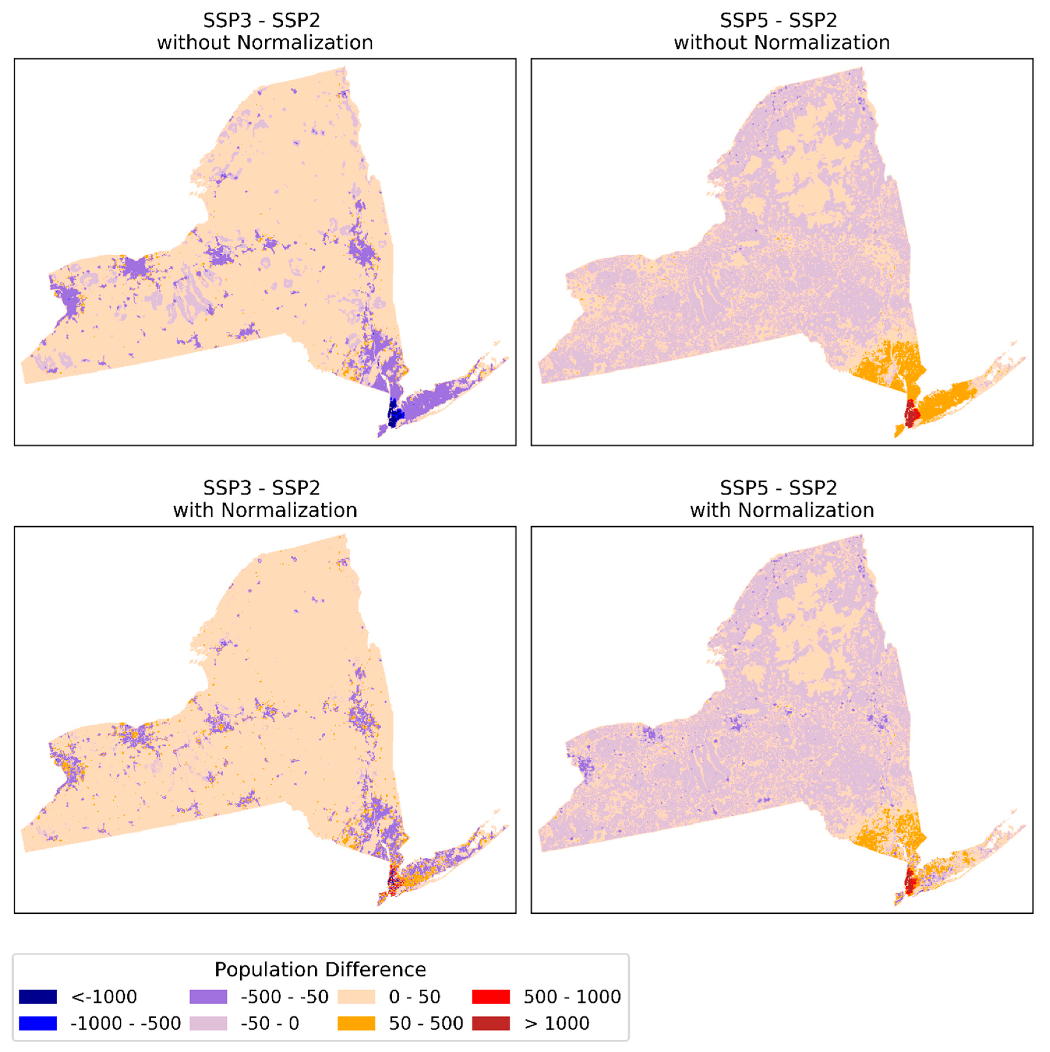
Appendix A.4. SSP Projections for New York

According to the state-level population projection model, the total population of the state of New York consistent with SSP2 increases gradually until 2050 and then decreases such that its population in 2100 is lower than its current value (Table A1). Under SSP5, the population of the state is projected to grow gradually to the point that it reaches ~26 million in 2100 whereas it continuously decreases consistent with SSP3 until it reaches ~11 million in 2100, significantly smaller than its current population.
Figure A6 and Figure A7 compare SSP3 and SSP5-based population grids of the state with its SSP2-based grids, with and without normalization, in 2050 and 2100, respectively. According to Figure A6, SSP3 leads to lower population than SSP2 broadly in urban areas (and in fact population decline in an absolute sense as well) whereas SSP5 results in higher population in suburban regions. Normalization reveals some specific effects of differences in spatial development patterns between scenarios. The lower urban population under SSP3 is concentrated in suburban areas, and population is actually higher in city centers. This is consistent with the SSP3 parameter values that preference population loss away from city centers, similar to the case for California in SSP3 described in the main text. Normalization also highlights the suburban population growth consistent with SSP5, pointing to the impact of its parameters consistent with sprawling development. However, the positive suburban population difference is limited to the surroundings of New York City, emphasizing New York City as the dominant socioeconomic hub of the state, reflected in the model as the highest suitability values are determined by nearby population concentrations. These effects are accentuated in 2100 according to Figure A7, where urban population decline under SSP3 is especially prominent (except for the central areas of New York City after normalization), and in SSP5 the rapid suburban population growth around New York City is noticeable (accentuated further in the normalized results, which in contrast to the suburbs show lower populations than SSP2 in the city center).
Figure A6. Population difference grids between SSP3, SSP5 and SSP2 in New York in 2050.
Sustainability 12 03374 g0a6
Figure A7. Population difference grids between SSP3, SSP5 and SSP2 in New York in 2100.
Sustainability 12 03374 g0a7

Appendix A.5. Regional Redistribution in State-Level Projections

The state-level projections produce a broad regional redistribution of population within the U.S. that is not easily captured in spatial downscaling models that downscale national level totals directly to grids. To illustrate the importance of representing the demographic processes that cause this redistribution (state-to-state migration as well as heterogeneity across states in other demographic rates), Figure A8 compares changes in state population from the state-level model [31] with those resulting from a model that downscales national totals directly to grid cells [17]. State level totals for this model are produced by aggregating projected grid cell outcomes to state boundaries [36]. This figure shows that in SSP2, the state-level model anticipates substantial regional variation in population growth across states, with some states declining in population. In contrast, downscaling national population totals directly to grid cells produces much less variation, without any states declining.
Figure A8. (a) Percentage of population change (2010–2100) consistent with SSP2 from the state-level projection model [31] (b) Percentage of population change (2010–2100) consistent with SSP2 after aggregating national population grids from the global model [17] to state boundaries [36].
Sustainability 12 03374 g0a8

Appendix A.6. Population Summary of Massachusetts and Utah

Table A4 presents population values of Massachusetts and Utah according to the global model (by aggregating the grids to their boundaries) [36] and state-level model [31] consistent with SSP2, SSP3 and SSP5 in 2100.
Table A4. Projected population aggregates of Massachusetts and Utah consistent with SSP2, SSP3 and SSP5 from the global and state-level models in 2100.
StateGlobal ModelState-Level Model
SSP2SSP3SSP5SSP2SSP3SSP5
Massachusetts106844146252805161905527771613442607411353269
Utah367286921347765609918644913239559168862053

References

  1. Meiyappan, P.; Dalton, M.; O’Neill, B.C.; Jain, A.K. Spatial modeling of agricultural land use change at global scale. Ecol. Modell. 2014, 291, 152–174. [Google Scholar] [CrossRef] [Green Version]
  2. Güneralp, B.; Seto, K.C. Futures of global urban expansion: Uncertainties and implications for biodiversity conservation. Environ. Res. Lett. 2013, 8, 014025. [Google Scholar] [CrossRef]
  3. Riahi, K.; Rao, S.; Krey, V.; Cho, C.; Chirkov, V.; Fischer, G.; Kindermann, G.; Nakicenovic, N.; Rafaj, P. RCP 8.5-A scenario of comparatively high greenhouse gas emissions. Clim. Chang. 2011, 109, 33. [Google Scholar] [CrossRef] [Green Version]
  4. Gao, J.; O’Neill, B.C. Data-driven spatial modeling of global long-term urban land development: The SELECT model. Environ. Model. Softw. 2019, 119, 458–471. [Google Scholar] [CrossRef]
  5. Shepard, C.C.; Agostini, V.N.; Gilmer, B.; Allen, T.; Stone, J.; Brooks, W.; Beck, M.W. Assessing future risk: Quantifying the effects of sea level rise on storm surge risk for the southern shores of Long Island, New York. Nat. Hazards 2012, 60, 727–745. [Google Scholar] [CrossRef]
  6. McGranahan, G.; Balk, D.; Anderson, B. The rising tide: assessing the risks of climate change and human settlements in low elevation coastal zones. Environ. Urban. 2007, 19, 17–37. [Google Scholar] [CrossRef]
  7. Xingong, L.; Rowley, R.J.; Kostelnick, J.C.; Braaten, D.; Meisel, J.; Hulbutta, K. GIS analysis of global impacts from sea level rise. Photogramm. Eng. Remote Sens. 2009, 75, 807–818. [Google Scholar]
  8. Jones, B.; O’Neill, B.C.; Mcdaniel, L.; Mcginnis, S.; Mearns, L.O.; Tebaldi, C. Future population exposure to US heat extremes. Nat. Clim. Chang. 2015, 5, 652–655. [Google Scholar] [CrossRef]
  9. Luber, G.; McGeehin, M. Climate Change and Extreme Heat Events. Am. J. Prev. Med. 2008, 35, 429–435. [Google Scholar] [CrossRef]
  10. Caminade, C.; Kovats, S.; Rocklov, J.; Tompkins, A.M.; Morse, A.P.; Colón-González, F.J.; Stenlund, H.; Martens, P.; Lloyd, S.J. Impact of climate change on global malaria distribution. Proc. Natl. Acad. Sci. USA 2014, 111, 3286–3291. [Google Scholar] [CrossRef] [Green Version]
  11. Hales, S.; De Wet, N.; Maindonald, J.; Woodward, A. Potential effect of population and climate changes on global distribution of dengue fever: An empirical model. Lancet 2002, 360, 830–834. [Google Scholar] [CrossRef]
  12. Monaghan, A.J.; Sampson, K.M.; Steinhoff, D.F.; Ernst, K.C.; Ebi, K.L.; Jones, B.; Hayden, M.H. The potential impacts of 21st century climatic and population changes on human exposure to the virus vector mosquito Aedes aegypti. Clim. Chang. 2018, 146, 487–500. [Google Scholar] [CrossRef]
  13. Striessnig, E.; Gao, J.; O’Neill, B.; Jiang, L. Empirically-based spatial projections of U.S. population age structure consistent with the shared socioeconomic pathways. Environ. Res. Lett. 2019, 14, 114038. [Google Scholar] [CrossRef]
  14. Byers, E.; Gidden, M.; Leclere, D.; Balkovic, J.; Burek, P.; Ebi, K.; Greve, P.; Grey, D.; Havlik, P.; Hillers, A.; et al. Global exposure and vulnerability to multi-sector development and climate change hotspots. Environ. Res. Lett. 2018, 13, 055012. [Google Scholar] [CrossRef] [Green Version]
  15. Jones, B.; O’Neill, B.C. Historically grounded spatial population projections for the continental United States. Environ. Res. Lett. 2013, 8, 044021. [Google Scholar] [CrossRef] [Green Version]
  16. McKee, J.J.; Rose, A.N.; Bright, E.A.; Huynh, T.; Bhaduri, B.L. Locally adaptive, spatially explicit projection of US population for 2030 and 2050. Proc. Natl. Acad. Sci. USA 2015, 112, 1344–1349. [Google Scholar] [CrossRef] [Green Version]
  17. Jones, B.; O’Neill, B.C. Spatially explicit global population scenarios consistent with the Shared Socioeconomic Pathways. Environ. Res. Lett. 2016, 11, 084003. [Google Scholar] [CrossRef]
  18. O’Neill, B.C.; Kriegler, E.; Ebi, K.L.; Kemp-Benedict, E.; Riahi, K.; Rothman, D.S.; van Ruijven, B.J.; van Vuuren, D.P.; Birkmann, J.; Kok, K.; et al. The roads ahead: Narratives for shared socioeconomic pathways describing world futures in the 21st century. Glob. Environ. Chang. 2017, 42, 169–180. [Google Scholar] [CrossRef] [Green Version]
  19. EPA. Updates to the Demographic and Spatial Allocation Models to Produce Integrated Climate and Land Use Scenarios (ICLUS) (Final Report, Version 2); US EPA: Washington, DC, USA, 2017. [Google Scholar]
  20. Bierwagen, B.G.; Theobald, D.M.; Pyke, C.R.; Choate, A.; Groth, P.; Thomas, J.V.; Morefield, P. National housing and impervious surface scenarios for integrated climate impact assessments. Proc. Natl. Acad. Sci. USA 2010, 107, 20887–20892. [Google Scholar] [CrossRef] [Green Version]
  21. Hauer, M.E. Population projections for U.S. counties by age, sex, and race controlled to shared socioeconomic pathway. Sci. Data 2019, 6, 190005. [Google Scholar] [CrossRef] [Green Version]
  22. KC, S.; Lutz, W. The human core of the shared socioeconomic pathways: Population scenarios by age, sex and level of education for all countries to 2100. Glob. Environ. Chang. 2017, 42, 181–192. [Google Scholar] [CrossRef] [PubMed] [Green Version]
  23. Jiang, L.; O’Neill, B.C. Global urbanization projections for the Shared Socioeconomic Pathways. Glob. Environ. Chang. 2017, 42, 193–199. [Google Scholar] [CrossRef] [Green Version]
  24. Dellink, R.; Chateau, J.; Lanzi, E.; Magné, B. Long-term economic growth projections in the Shared Socioeconomic Pathways. Glob. Environ. Chang. 2017, 42, 200–214. [Google Scholar] [CrossRef]
  25. Hasegawa, T.; Fujimori, S.; Takahashi, K.; Masui, T. Scenarios for the risk of hunger in the twenty-first century using Shared Socioeconomic Pathways. Environ. Res. Lett. 2015, 10, 014010. [Google Scholar] [CrossRef]
  26. Merkens, J.L.; Reimann, L.; Hinkel, J.; Vafeidis, A.T. Gridded population projections for the coastal zone under the Shared Socioeconomic Pathways. Glob. Planet. Chang. 2016, 145, 57–66. [Google Scholar] [CrossRef] [Green Version]
  27. Nauels, A.; Rogelj, J.; Schleussner, C.F.; Meinshausen, M.; Mengel, M. Linking sea level rise and socioeconomic indicators under the Shared Socioeconomic Pathways. Environ. Res. Lett. 2017, 12, 114002. [Google Scholar] [CrossRef] [Green Version]
  28. Rohat, G. Projecting drivers of human vulnerability under the shared socioeconomic pathways. Int. J. Environ. Res. Public Health 2018, 15, 554. [Google Scholar] [CrossRef] [Green Version]
  29. Zoraghein, H.; O’Neill, B.C. The methodological foundation of a gravity-based model to downscale U.S. state-level populations to high-resolution distributions for integrated human-environment analysis. Demogr. Res. under review.
  30. Grübler, A.; O’Neill, B.; Riahi, K.; Chirkov, V.; Goujon, A.; Kolp, P.; Prommer, I.; Scherbov, S.; Slentoe, E. Regional, national, and spatially explicit scenarios of demographic and economic change based on SRES. Technol. Forecast. Soc. Chang. 2007, 74, 980–1029. [Google Scholar]
  31. Jiang, L.; O’Neill, B.; Zoraghein, H.; Dahlke, S. Population scenarios for U.S. states consistent with Shared Socioeconomic Pathways. Environ. Res. Lett. under review.
  32. Zoraghein, H.; Jiang, L. The Improved Urbanization Projections of the NCAR Community Demographic Model (CDM). NCAR Tech. Notes 2018. [Google Scholar] [CrossRef]
  33. Zoraghein, H.; O’Neill, B. Data Supplement: U.S. State-Level Projections of the Spatial Distribution of Population Consistent with Shared Socioeconomic Pathways. (Version v0.1.0) [Data set]. Available online: https://doi.org/10.5281/zenodo.3756179 (accessed on 19 April 2020).
  34. Zoraghein, H.; O’Neill, B.C.; Vernon, C. Population Gravity Model (Version v0.1.0). Available online: https://github.com/IMMM-SFA/population_gravity. (accessed on 19 April 2020).
  35. Santos, A.; McGuckin, N.; Nakamoto, H.Y.; Gray, D.; Liss, S. Summary of Travel Trends: 2009 National Household Travel Survey; U.S. Department of Transportation: Washington, DC, USA, 2011. [Google Scholar]
  36. Jiang, L.; Zoraghein, H.; O’Neill, B.C. Population projections for US states under the Shared Socioeconomic Pathways based on global gridded population projections. NCAR Tech. 2018. [Google Scholar] [CrossRef]
  37. Gao, J. Downscaling Global Spatial Population Projections from 1/8-degree to 1-km Grid Cells. NCAR Tech. Notes 2017. [Google Scholar] [CrossRef]
Figure 1. High-level illustration of the gravity-based model.
Sustainability 12 03374 g001
Figure 2. The influence of α and β on the suitability of a focal cell.
Sustainability 12 03374 g002
Figure 3. Population projection grids for the contiguous U.S. according to SSP2, SSP3, and SSP5 in 2050 (top panels) and in 2100 (bottom panels).
Sustainability 12 03374 g003
Figure 4. Population difference grids between the SSP3, SSP5, and SSP2 in 2050 and 2100.
Sustainability 12 03374 g004
Figure 5. Population difference grids between SSP3, SSP5, and SSP2 in California and in 2050 (left panels) and 2100 (right panels), with and without normalization.
Sustainability 12 03374 g005
Figure 6. Population difference grids between the national and global models across SSP2, SSP3, and SSP5 with and without normalization for the contiguous U.S. in 2100.
Sustainability 12 03374 g006
Figure 7. Population difference grids between the state-level and global models across SSP2, SSP3, and SSP5 with and without normalization for Massachusetts in 2100.
Sustainability 12 03374 g007
Figure 8. Population difference grids between the state-level and global models across SSP2, SSP3, and SSP5 with and without normalization for Utah in 2100.
Sustainability 12 03374 g008

