Article

The Price-Volume Relationship of the Shanghai Stock Index: Structural Change and the Threshold Effect of Volatility

1
School of Finance, Zhejiang Gongshang University, Hangzhou 310018, China
2
College of Management, National Taiwan Normal University, Taipei 106, Taiwan
3
School of Economics and Management, Tongji University, Shanghai 200092, China
*
Author to whom correspondence should be addressed.
Sustainability 2020, 12(8), 3322; https://doi.org/10.3390/su12083322
Submission received: 22 March 2020 / Revised: 14 April 2020 / Accepted: 17 April 2020 / Published: 19 April 2020
(This article belongs to the Section Economic and Business Aspects of Sustainability)

Abstract

:
The price–volume relationship of stocks can be impacted substantially by structural changes and market volatility. In this paper, we analyze China’s stock market behavior and subsequent price–volume equation, with emphasis on two periods of market volatility and structural changes during 2007–2008 and 2015–2016. To account for the impacts of unknown volatility and time breaks, we embed the price–volume relationship into a vector autoregression (VAR) framework with structural breaks and volatility thresholds. Our results indicate that significant time-breaking effects exist and that the high-low volatility effects are substantial. Finally, in its entirety, we identify only a linear causal relationship from price to volume.

1. Introduction

Research on the relationship between stock price and trading volume is one of the most important components of technical analysis of the stock market. It is also a key issue in the field of financial market prediction and risk management. The dramatic behavior of China’s stock market in recent years, especially during the two periods of considerable volatility in the years 2007–2008 and 2015–2016, may have substantially affected the price–volume relationship by structural change and market volatility. Previous studies have examined the dynamic price–volume relationship through the application of a VAR framework. However, the conventional VAR approach to the dynamics of price–volume relations fails to account for the impacts of structural change and market volatility, which are regular features of China’s stock markets. To this end, this study contributes to the literature by assessing the price–volume relationship of China’s stock market using a VAR framework with structural break and volatility thresholds.

2. Literature Review

As discussed by Karpoff [1], the relationship between financial asset returns and trading volume (price–volume relation) reveals important insights into the operational efficiency and information dynamics in asset markets. Both Karpoff [1] and Gallant et al. [2] point out that previous empirical work has focused mainly on the contemporaneous relationship between price change and volume. Yet, as far as prediction and risk management are concerned, studying the dynamic (causal) relationship between returns and volume is more informative [3].
Some studies have theoretically investigated the dynamic relationship between trading volume and stock returns, which may have some causal relationship implications. Copeland [4] and Jennings et al. [5] derived the information arrival model and suggest a positive causal relationship between stock returns and trading volume in both directions. In the mixture of distributions model of Epps and Epps [6], trading volume is used to measure disagreements, as traders revise their reservation prices based on the receipt of new market information. The greater the extent of disagreement among traders, the higher the trading volume. Their model suggests a positive causal relationship running from trading volume to absolute returns. In Clark’s [7] mixture model, trading volume is a proxy for the speed of information flow, which is a latent common factor affecting contemporaneous stock returns and volume. There is, however, no causal relation from trading volume to stock returns in Clark’s common factor model [7]. Campbell et al. [8] present a model which implies that price changes accompanied by high volume will tend to be reversed, and this will be less true of price changes on days with low volume. There are also equilibrium models that emphasize the information content of volume. Blume et al. [9] stress that volume provides data on the quality or precision of information on prior price movements, and hence is useful for interpreting the price (return) behavior. Wang [10] analyzes dynamic relationships between volume and returns on a model with information asymmetry, which shows that volume may provide information about future returns. Liu et al. [11] find that the aggressive trading style of informed agents can produce a price–volume relationship in an agent-based model with information asymmetry. Based on the Kelly criterion of asset allocation, Wang and Yang [12] present a price–volume model that shows the accumulated absolute deviation of a risk asset’s return from its risk-free rate is related with its trading volume.
Despite strong theoretical underpinnings and a thorough survey of empirical evidence, Karpoff [1] finds that the contemporaneous correlation between price changes and trading volume is both mixed and weak. Gallant et al. [2] also find the same. Since the 1990s, focus has moved to dynamic (causal) stock return–volume relationships which are mainly based on the Granger causality test. Related to this study, the even theoretically well-grounded notion of causality from past trading volume to returns, does not find strong empirical support either. For instance, Lee and Rui [13] report that trading volume does not predict returns for the next day in Chinese A and B markets in Shanghai and Shenzhen. Chen et al. [14] report no causal link in France, Italy, Japan, the UK or the US. Lee and Rui [15], using daily data, find that trading volume does not Granger-cause stock market returns on each of the US, Japanese and UK stock exchanges. Volume–returns causality is neither found by Rashid [16] for Pakistan, nor by Pisedtasalasai and Gunasekarage [17] for five south-east Asian emerging markets. Azad et al. [18] investigate the price–volume relation in three south Asian stock markets and find that there exists a weak form of market inefficiency in those markets. Chuang et al. [19] find volume to cause returns in only two out of the ten Asian markets analyzed. Wang et al. [20] investigate the US stock market return–volume relation from the perspective of out-of-sample stock return predictability, and the result shows that higher returns do follow more intensive trading. Chen [21] shows S&P 500 trading activity affects subsequent returns only in bear markets –but exhibits no volume-return causality when both market phases are considered jointly. Using a cross-country dataset consisting 13 major global stock indices, Patra and Bhattacharyya [22] find that volume cannot explain the heteroscedasticity of return. However, some studies do establish the existence of volume-return causality, for example, Saatcioglu and Starks [23] and Rojas and Kristjanpoller [24] for six Latin American countries. Rzayev and Ibikunle [25] decompose trading volume into liquidity-driven and information-driven components. Using a high-frequency S&P 500 stock dataset, they show that the latter is a statistically significant predictor of one-second stock returns.
A nonlinear relationship between volume and subsequent returns garners some empirical support [21,26]. A recent paper by Chuang et al. [3] uses quantile regressions to report that for the NYSE, S&P 500 and FTSE 100 indices, past trading volume exerts a positive (negative) impact on returns from the top (bottom) of return distribution. Lin [27], using the same methodology, confirms these findings for six emerging markets. Gebka and Wohar [28] use quantile regression to show that for a set of mature and emerging Pacific Basin countries, positive (negative) volume-return causality in high (low) return quantiles is not limited to one market but seems to be a common feature across countries. Matilla-García et al. [29] investigate the volume-stock price relation using the method of non-parametric testing based on permutation entropy. Hasan and Salim [30] and El Alaoui [31] use multifractal detrended fluctuation analysis (MF-DFA) and multifractal detrended cross-correlation analysis (MF-DCCA) methods to report cross-correlations between price and volume change. Gupta et al. [32] use the Maximum Overlap Discrete Wavelet Transform (MODWT)-VAR approach to examine the price–volume relation in China and India’s stock markets; the relationship is found to vary across different time horizons. Using a nonlinear Granger causality testing framework, Kyrtsou et al. [33] show that the return–volume relationship for S&P 500 is asymmetric. Wang et al. [34] use the dependence-switching copula model to examine the price–volume dependence structure across six major international stock markets; the result shows that the price–volume dependence is asymmetric. In a model of stochastic volatility with volume (SV-VOL), Chen et al. [35] find that the exchange-market volume information affects the stock market price–volume relationship. Using evidence from the Korean stock market, Chae and Kang [36] analyze the influence of abnormal trading volumes on post-event returns and find low-volume return premiums in the Korean stock market. Ülkü and Onishchenko [37] show that the predictive role of trading volume for short-horizon reversals in stock returns can be contrasting by conditioning on different investor types’ trading.
The methodology of the extant literature to investigate the relation between price and trading volume, no matter linear or nonlinear, rarely considers the impacts of structural change and market volatility (or market uncertainty), which are common features in China. This paper argues that, if we use trading volume to measure investors’ trading behavior, then the price–volume relationship can be interpreted as the bidirectional interaction between trading behavior and market price. On the one hand, investors make trading decisions based on their expectations of the future stock price. On the other hand, their trading behavior, in turn, affects the market price. An important fact that should not be ignored is that investors make trading decisions based on their expectations of future price, which means investors make trading decisions in an uncertain environment. Therefore, when making trading decisions, investors not only consider the expected stock price, but they also take the uncertainty of the future price (i.e., the risk, which can be measured by volatility) into account. Even at the same expected price, the difference in price uncertainty may lead investors to make rather different trading decisions. Thus, the price–volume relationship could very possibly be affected by market uncertainty. In particular, due to the frequent volatility of the Chinese stock markets, the impact of market uncertainty on the price–volume relationship could be substantial.
Furthermore, due to the short history of China’s stock market, it is far from being a mature and effective capital market. Hence, the stability of China’s stock market is relatively poor compared to those of mature markets. Dramatic fluctuations frequently occur in China’s stock market, such as the two periods of considerable volatility in the years of 2007–2008 and 2015–2016, which may contribute to significant time-breaking effects on price–volume dynamics, leading the price–volume relationship in China’s stock market to exhibit a much more complicated structural change characteristic compared to mature markets.
This study contributes to the literature by applying a threshold VAR approach to investigate the impacts of market volatility and structural change on the price–volume relation. To account for the impacts of unknown volatility and time breaks, we embed the price–volume relation in a VAR framework with structural change and volatility thresholds. The rest of the paper is organized as follows: Section 3 presents the details of the linear and threshold VAR approach. Then we outline the data in Section 4; after which we explicitly detail our empirical results in Section 5. Section 6 concludes the paper.

3. Methodology

3.1. Linear VAR

According to previous literature, there exists a bidirectional causality between price and volume, so modeling the price–volume relationship would encounter the problem of endogeneity. The VAR method, which constructs the model by treating each endogenous variable as a function of the lagged values of all endogenous variables [38], is an effective instrument for tackling the problem of endogeneity. The ordinary VAR approach assumes linearity in the model, thus it is also called linear VAR.
We first use the linear VAR approach to investigate the overall price–volume relation of China’s stock market. Letting t denote the time index, we set stock returns ( r e t t ) and trading volume ( v o l t ) as the explained variables of the two regression equations, denoted by { v o l t , r e t t } t = 1 T . The p-order-lagged values of the two variables are used as the explanatory variables, thus forming a binary VAR (p) system:
[ v o l t r e t t ] = [ c 1 c 2 ] + L i [ a 1 i b 1 i a 2 i b 2 i ] [ v o l t i r e t t i ] + [ ε 1 t ε 2 t ]
In Equation (1), v o l t i and r e t t i are auto regression (AR) terms. a 1 i and b 1 i , a 2 i and b 2 i are the coefficients of AR terms in the two equations. L i is the lag operator, where i=1, 2,..., p. c 1 and c 2 are constant terms and ε 1 t and ε 2 t are disturbance terms.

3.2. Threshold VAR

The threshold VAR (TVAR) approach is an extended VAR model that identifies the nonlinear features in the VAR system. The nonlinearity may emerge from structural change or other asymmetric effects. For the research object of this study, nonlinearity is taken to mean that the price–volume relationship could be affected by certain feature variables. The feature variable is called a threshold variable which can be used to divide the sample. The dividing criterion set by the threshold variable is the threshold value, according to which the original sample can be divided into several subsamples. The model nonlinearity captured by the threshold variable allows the coefficient matrix of the model to change in different subsamples. The threshold variable can either be an endogenous variable of the VAR system or another exogenous variable. The threshold value can be set to one or more, and the sample can thus be divided into two or more subsamples.
Assuming that the sample data are { v o l t , r e t t , t h v t } t = 1 T , where t h v t denotes the threshold variable. Then the mathematical expression of the TVAR model is shown as follows:
[ v o l t r e t t ] = I ( t h v t γ ) ( [ c 1 c 2 ] + L i [ a 1 i b 1 i a 2 i b 2 i ] [ v o l t i r e t t i ] ) + I ( t h v t > γ ) ( [ c 1 c 2 ] + L i [ a 1 i b 1 i a 2 i b 2 i ] [ v o l t i r e t t i ] ) + [ ε 1 t ε 2 t ]
In Equation (2), I(·) is an indicative function, which is equal to 1 if the expression in parentheses is true and 0 otherwise. γ is the threshold value to be estimated. It can be seen that the TVAR model is a nonlinear model because it cannot be expressed as a linear function of each parameter. The estimation methodology of the TVAR model is in minimizing the sum of square residuals (SSR), where a two-step approach is used: first, taking the value of γ as given, use a linear regression approach to estimate the coefficients of Equation (2) and then calculate the sum of squared residuals SSR( γ ), which is a function of γ . Second, choose γ to minimize SSR( γ ) and the coefficients can be estimated accordingly.
The likelihood ratio (LR) testing approach can be used to test the significance of the threshold effect [39]:
LR = [ S S R * S S R ( γ ^ ) ] / σ ^ 2
The null hypothesis ( H 0 ) of the LR test is, “There exists no threshold effect”. S S R * is the sum of squared residuals under H 0 (that is, linear VAR). S S R ( γ ^ ) is the sum of the squared residuals of the TVAR estimation result. σ ^ 2 is the consistent estimator of the variance of the disturbance term. The larger the value of S S R * S S R ( γ ^ ) , the more the SSR is increased under H 0 , and the more it tends to reject H 0 .
Similarly, when setting two threshold values (i.e., γ 1 and γ 2 , γ 1 < γ 2 ), the TVAR model can be expressed as shown in Equation (4):
[ v o l t r e t t ] = I ( t h v t γ 1 ) ( [ c 1 c 2 ] + L i [ a 1 i b 1 i a 2 i b 2 i ] [ v o l t 1 r e t t 1 ] ) + I ( γ 1 < t h v t γ 2 ) ( [ c 1 c 2 ] + L i [ a 1 i b 1 i a 2 i b 2 i ] [ v o l t 1 r e t t 1 ] ) + I ( t h v t > γ 2 ) ( [ c 1 c 2 ] + L i [ a 1 i b 1 i a 2 i b 2 i ] [ v o l t 1 r e t t 1 ] ) + [ ε 1 t ε 2 t ]
The key to constructing a TVAR model lies in the selection of the threshold variables. With the selection of different threshold variables, both the estimation results and their implications are different. When setting a deterministic time dummy as a threshold variable ( t h v t = t ), we can examine the structural change characteristics of the VAR system [40].

3.3. Research Design

We first model the price–volume relationship of China’s stock market in a linear VAR framework, and then use the Granger causality test to investigate the overall characteristics of the price–volume relationship. Second, we construct a TVAR model with a time threshold ( t h v t = t ). Based on the estimated time threshold values, we divide the sample into several subsamples, in which the Granger causality test is performed in detail, to identify the structural change characteristics of the price–volume relationship. Finally, market volatility is used as a threshold variable ( t h v t = σ r e t , t 2 ) to construct a TVAR model to examine the asymmetric impacts of market uncertainty on the price–volume relationship.

4. Data

The daily data of closing price ( P t ) and trading volume ( Q t ) of the Shanghai Stock Index from March 4, 2003 to April 22, 2019 were collected. The number of sample observations was 3923. The original data were processed as follows: first, calculate the daily return ( r e t t ) of the Shanghai Stock Index according to Equation (5); second, detrend the trading volume series according to regression Equation (6), in which T is the time variable and then filter the regression residual term out and use it as the adjusted volume ( v o l t ).
r e t t = [ log ( P t ) log ( P t 1 ) ] 100
log ( Q t ) = c + α T + ε
We use price volatility to measure market uncertainty. Fit ret t with the GARCH (1,1) model as shown in Equation (7), then filter σ r e t , t 2 out and use it as the measure of market volatility.
{ Mean   Equation :   ret t = c + ϕ ret t 1 + ε t Variance   Equation :   σ r e t , t 2 = ω + α ε t 1 2 + β σ r e t , t 1 2
The time series plots for all variables are shown in Figure 1. As can be seen, there exists a clear positive correlation between the price and trading volume of the Shanghai Stock Index; it was particularly significant during the period of the two extreme volatilities in 2007–2008 and 2015–2016. However, the major distinction between the two volatility periods was that the extent of variation of trading volume in 2015–2016 was more drastic than in 2007–2008. The market displays a noteworthy feature of volatility clustering, with high volatility periods mainly clustering during 2007–2008 and 2015–2016. In those periods, the variability of price and volume was also relatively high, which was likely to cause structural changes in the price–volume relationship.
Table 1 shows the results for descriptive statistics. Both price series before and after adjustment have kurtosis characteristics. The original price series was right skewed, and the adjusted one was left skewed. Both volume series, before and after the adjustment show kurtosis features and were right skewed. The J-B test significantly rejects the normal distribution hypothesis for all variables, which indicates that all these time series were skewed during the sample period. The ADF test shows that both adjusted price and volume series have no unit roots, thus satisfying the conditions for VAR modeling.

5. Empirical Results and Discussion

5.1. Overall Price-Volume Relationship in China’s Stock Market

According to the Schwartz Information Criterion (SIC), the optimal lag order of the VAR model was determined to be 6. Therefore, we construct a VAR (6) model based on Equation (1). The Granger causality test result (Table 2) shows that price was the Granger cause of volume at the 0.1% significance level. Trading volume was also the Granger cause of price, but with significance level only at 5%. Given that the sample size was relatively large, 5% significance level was not that persuasive. Therefore, it can be inferred that the price of the China stock market significantly affects trading volume during 2003–2019, while the reverse impact of volume on price was much weaker.

5.2. Test of Structural Change

5.2.1. Estimation of Time Thresholds

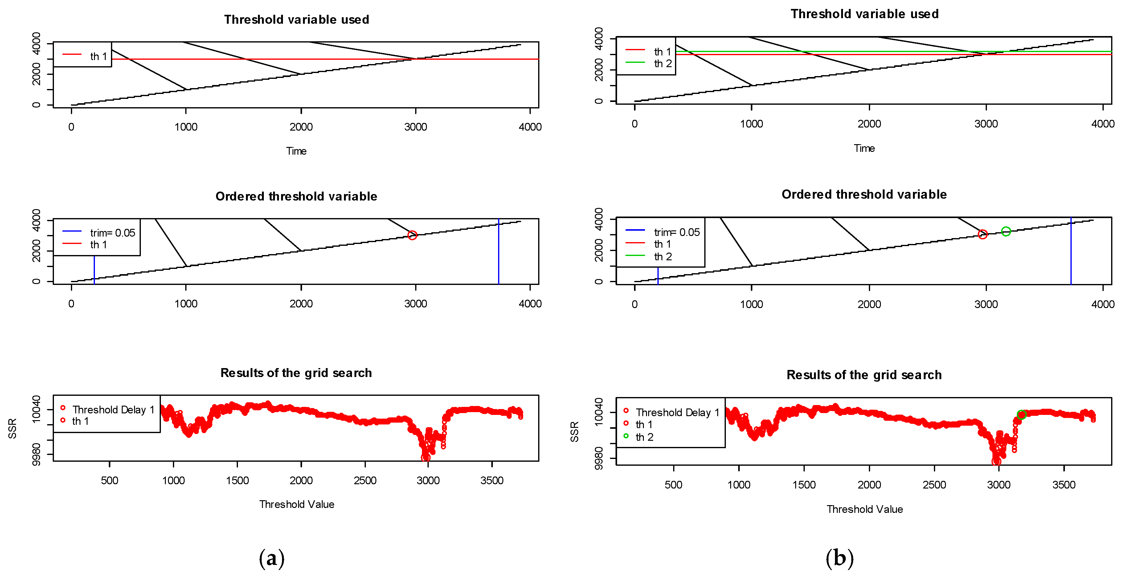
According to Equation (2) and/or Equation (4), we construct a TVAR model with time as the threshold variable ( t h v t = t ). The selection process of time threshold values is shown in Figure 2, where the upper graphs are the time plots of the threshold variable (Since the time is a kind of special threshold variable, its sequence diagram is an upward sloping straight line.); the middle graphs show the ordering of the threshold variable; and the lower ones give the results of the grid search (The horizontal axis shows the threshold value searched out, and the vertical axis shows the sum of squared residuals (SSR).). The estimating and testing results of the TVAR model are listed in Table 3A. When a single threshold value was set, the estimated threshold value was t = 2015/06/11, and the LR statistics of both equations in the TVAR system reject the null hypothesis of “no threshold effect” at a 0.1% significance level, indicating that there exists significant structural break effect for the price–volume relation at t=2015/06/11. When two threshold values were set, the estimated threshold values were t1=2015/06/11 and t2=2016/03/31; the estimation result passes the LR test as well.
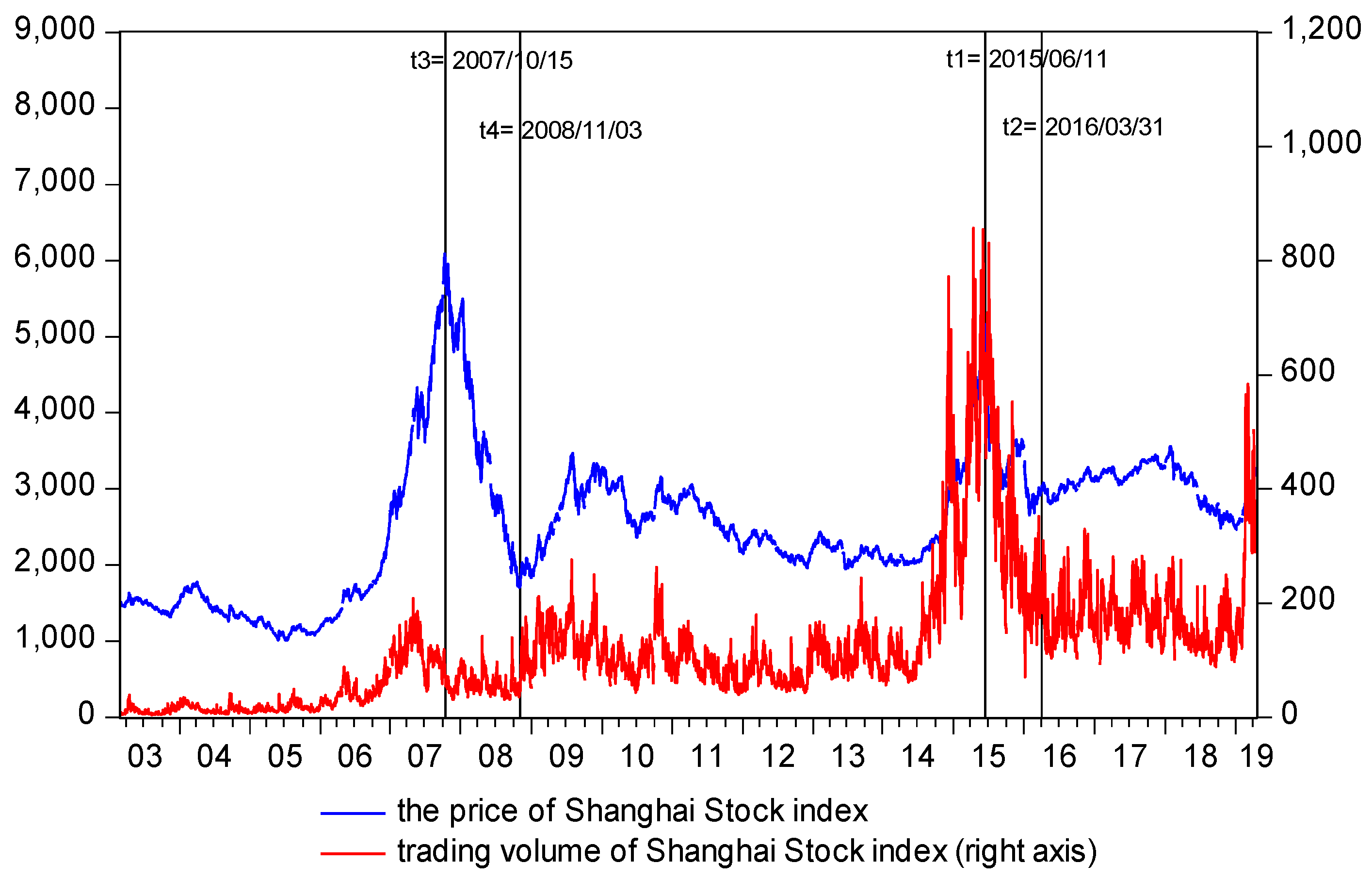
The estimation result of the TVAR model matches the trend of China’s stock market quite well. Two threshold values, t1 and t2, exactly identify the bull and bear cycle of 2015–2016. At t1, the Shanghai Stock Index rose to its highest level at 5121 before it began to slump all the way down to the lowest level of 1707 at t2.
t1 and t2 divide the original sample period into three sub-ranges, namely 2003/03/04–2015/06/11, 2015/06/11–2016/03/31 and 2016/03/31–2019/4/22. Since the time span of the sub-range 2003/3/4–2014/8/28 was relatively long, and it contains a complete bull and bear cycle, the price–volume relation could have also encountered significant structural changes during this period. Therefore, we construct the TVAR model again for the sub-range 2003/3/4–2015/06/11. The estimating and testing results are shown in Table 3B. The single threshold value estimated was t’=2007/10/15, and the two threshold values estimated were t3=2007/10/15 and t4=2008/11/03. All estimation results pass the LR test, which suggests that there exist significant structural breaking effects at t3 and t4.
The estimation result of the TVAR model based on sample range 2003/3/4–2015/06/11 also matches the trend of China’s stock market very well. Two threshold values, t3 and t4, exactly identify the bull and bear cycle of 2007–2008. At t3, the Shanghai Stock Index rose to a historical high level of 6030 before it began to slump all the way down to the lowest level of 1719 at t4.
So far, we have identified four, time threshold values (Figure 3)—t1, t2, t3 and t4—at which significant structural changes of the price–volume relationship occurred. According to the sequence of the four, time threshold values being identified, the significance of structural changes at t1, t2, t3 and t4 can be ordered as t1>t2>t3>t4. Therefore, it can be inferred that: it was usually during the period of the stock market crash when the price–volume relationship significantly changes. Second, when the stock market begins to slump after reaching a peak, the degree of structural change was more significant (t1>t2, t3>t4). Third, the structural changes in the price–volume relationship in 2014–2015 was more significant than in 2007–2008.

5.2.2. The structural Change Characteristics of the Price-Volume Relation

According to t1, t2, t3 and t4, the original sample can be divided into five subsamples, in which we can, respectively, construct the linear VAR. Granger causality test results (Table 4) in a linear framework show that only in subsample 1 does the trading volume Granger cause price change. That is, trading volume has a certain effect on the price only before the stock market collapse in 2007; after that the effect was no longer significant. On the contrary, the effect of price on trading volume was always highly significant except for in subsample 4.
Therefore, it can be inferred that the impact of price on trading volume in China’s stock market was far larger than in the opposite direction; thus, the market was mainly driven by price, rather than trading volume.

5.3. The Threshold Effect of Market Volatility on Price-Volume Relation

5.3.1. Estimation of Volatility Thresholds

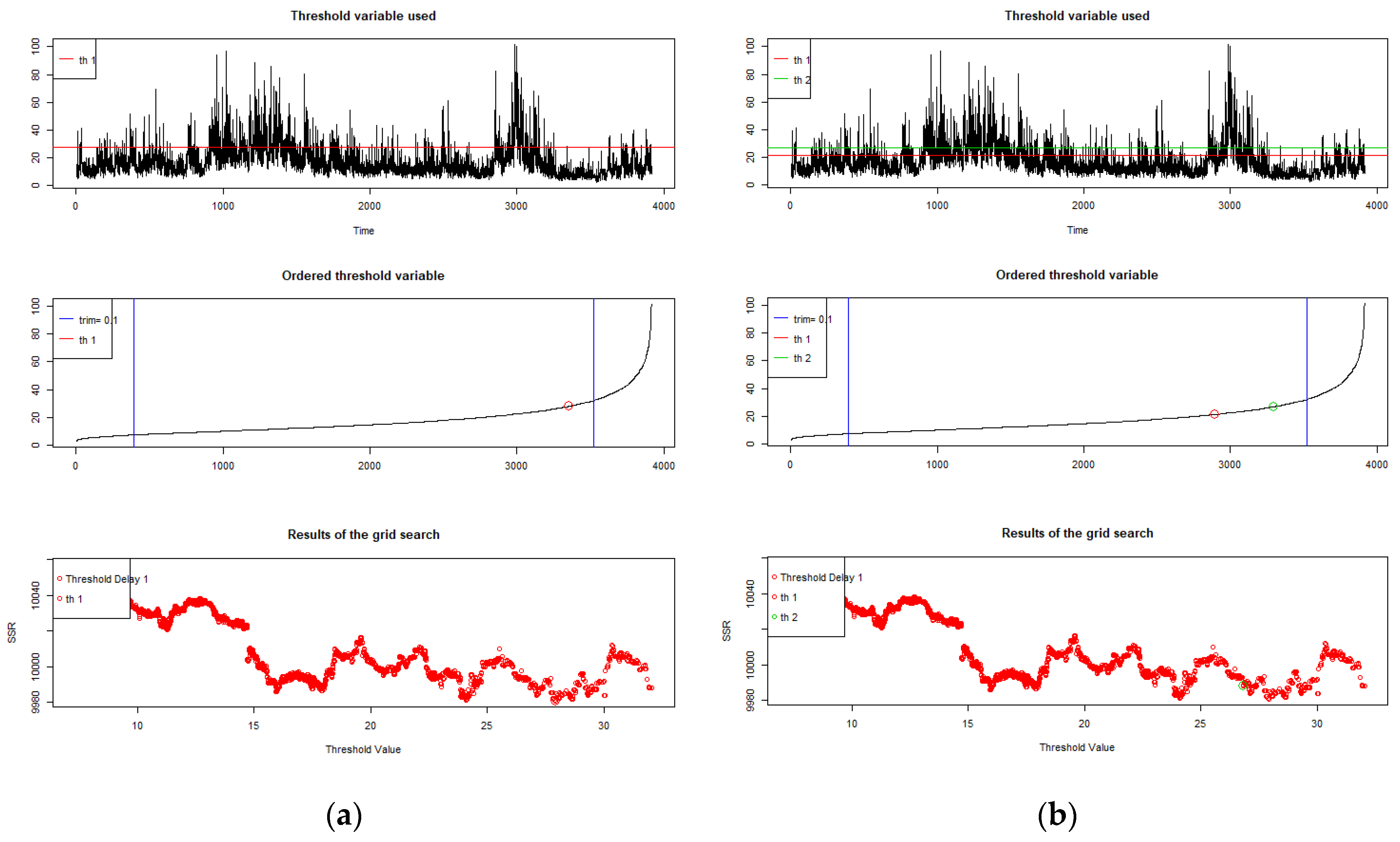
According to Equation (2) and/or Equation (4), we construct a TVAR model with the level of market volatility as a threshold variable ( t h v t = σ r e t , t 2 ). The selection process of volatility threshold values is shown in Figure 4. The upper graph in Figure 4 contains the time plots of the threshold variable, which is the same as Figure 1E. The middle and the lower graphs in Figure 4 reflect the ordering of the threshold variable and the results of a grid search, respectively. The estimating and testing results of the TVAR model are listed in Table 5. The single threshold value estimated was σ r e t , t 2 =6.52 and the two threshold values estimated were σ r e t , t 1 2 =3.09 and σ r e t , t 2 2 =6.52. All estimation results pass the LR test, indicating that there exist significant threshold effects at σ r e t , t 1 2 and σ r e t , t 2 2 .
The estimation results of the TVAR model match the trend of China’s stock market quite well. As can be seen from Figure 4A, most of the observations of the subsample σ r e t , t 2 > 6.52 were clustering in the periods of 2007–2008 and 2015–2016 when large movements in the stock market occurred; which indicates that the price–volume relationship has changed significantly during the two periods of considerable market volatility. When two threshold values were set (Figure 4b), the estimation result further divides the subsample σ r e t , t 2 6.52 into two subsamples, namely, 3.09 < σ r e t , t 2 6.52 and σ r e t , t 2 3.09. The subsample 3.09 < σ r e t , t 2 6.52 mainly contains periods of relatively higher volatility in the periods other than 2007–2008 and 2015–2016, which further indicates that the change in market volatility significantly impacts price–volume relationship.

5.3.2. The Threshold Effect of Market Volatility on the Price-Volume Relationship

According to the volatility threshold values estimated, the original sample can be divided into several subsamples. However, due to the discontinuity of observations in each subsample, the Granger causality test in the linear VAR framework cannot be performed in each subsample. Instead, we compare the changes of coefficient (and significance level) of the explanatory variable in different subsamples of the TVAR system, to identify the asymmetric impact of market volatility on the price–volume relationship. In a TVAR (6) system, the price and volume of lags 1 to 6 are used as explanatory variables. Due to the strong auto-correlation among lagged variables, it was difficult to interpret the implication of coefficients (and significance levels) of all the lagged variables. In general, the price and volume of the day before has the highest impact on the price and volume of the day. The more days apart, the lower the impact was. In other words, the 1-order-lagged explanatory variable has the highest impact on the explained variable, so the coefficient and significance level of the 1-order-lagged explanatory variable were the most credible and persuasive. Therefore, we choose to compare the changes in coefficients (and significance levels) of 1-order-lagged prices and volumes in different subsamples, to identify the impact of volatility on the price–volume relationship.
The regression result of the TVAR model is shown in Table 6. We first compare the changes in the coefficient of vol(-1) in equation ret; in subsample σ r e t , t 2 6.52 , the coefficient of vol(-1) was 0.3953 at the 1% significance level. However, as market volatility increases, in subsample σ r e t , t 2 > 6.52 the coefficient of vol(-1) was no longer significant.
Then we compare the changes in the coefficient of ret(-1) in equation vol; in subsample σ r e t , t 2 3.09 the coefficient of ret(-1) was 0.0515 at a 0.1% significance level. As market volatility increases, in subsample 3.09 < σ r e t , t 2 6.52 and subsample σ r e t , t 2 > 6.52 , the coefficient of ret(-1) decreases to 0.0328 and 0.0199, respectively, while still highly significant at 0.1% level.
Therefore, it can be inferred that trading volume only slightly impacts price when market volatility level was relatively low, while the price significantly impacts trading volume at any time. With the increase of volatility level, the impact of trading volume on price gradually disappears, while the impact of price on volume still remains highly significant, but with a gradual decline in economic significance. The above findings confirm our conjecture in Section 1—market uncertainty (volatility) significantly affects the price–volume relationship. Since investors make their trading decisions in an uncertain environment, trading decisions of investors depend not only on their expectations of future stock price but were also affected by price uncertainty (volatility).

5.4. Robustness Checks

In this section, we examine the robustness of our results to the selection of volatility estimators. In the above empirical analysis, we use the market volatility estimated via the GARCH model. To check whether our results are sensitive to other types of volatility estimators, we use two alternative range-based volatility estimators— σ r e t , t 2 P proposed by Parkinson [41] and σ r e t , t 2 G K proposed by Garman and Klass [42]. These two estimators are defined as follows:
σ r e t , t 2 P = 1 4 l n 2 ( H t L t ) 2
and
σ r e t , t 2 G K = 0.511 ( H t L t ) 2 0.019 [ ( C t O t ) ( H t + L t 2 O t ) 2 ( H t O t ) ( L t O t ) ] 0.383 ( C t O t ) 2
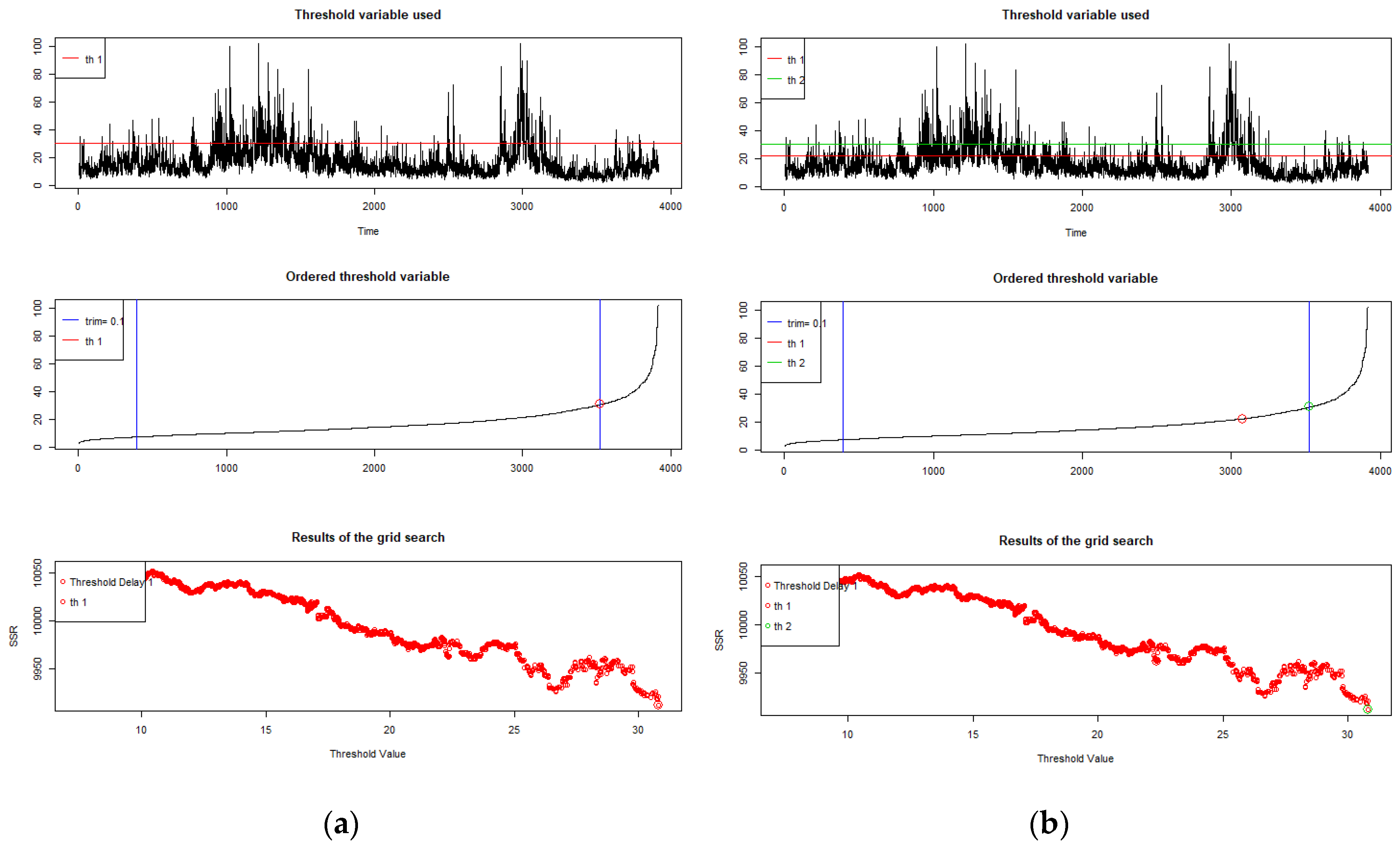
In Equations (8) and (9), H t , L t , O t and C t are the natural logarithms of the daily high, low, opening and closing prices of the Shanghai Stock index. Figure 5 and Figure 6 show the selection process of volatility thresholds using the two alternative volatility estimators above. Table 7 and Table 8 show the regression result of the TVAR model using these two estimators. The overall qualitative patterns of the dynamic price–volume relationship in different volatility subsamples using the two range-based volatility estimators ( σ r e t , t 2 P and σ r e t , t 2 G K ) are similar to those observed using the GARCH volatility ( σ r e t , t 2 ). With the increase in volatility level, the impact of volume on price gradually disappears, while the impact of price on volume remains highly significant, but with a gradual decline in economic significance. This indicates that our results are robust to different volatility estimators.

6. Conclusions

In literature, the empirical price–volume relationship is examined in a VAR framework. However, the conventional VAR approach to the dynamics of price–volume relations fails to account for the impacts of structural changes and volatility levels, which commonly occur in China. This study contributes to the literature by estimating the price–volume relation in the VAR framework with structural changes and volatility thresholds. As a result, we obtain the following evidence: first, the evidence indicates that there exist significant time-breaking effects in the two periods of considerable volatility in 2007–2008 and 2015–2016, and the structural change in the latter period was more significant. Second, the high-low volatility effects are substantial. When the level of volatility was relatively low, price and volume affect each other. As volatility level increases, the impact of volume on price gradually disappears; while the impact of price on volume remains highly significant, its economic significance has also declined. Finally, as a whole, we identify only a linear causal relation from price to volume. Rather than a volume-driven market, this shows that China’s stock market was mainly driven by yield.
The findings of this study are of significance for global investors to better understand the microstructure of China’s stock market and its structural change characteristics. As an emerging market, China’s stock market is far from mature compared to those of industrialized economies. The basic issuance and trading system and the investor structure of the Chinese stock market have been constantly changing in recent years and are still far from reaching the stable level of mature markets. This is likely to be the reason for the significant structural change effects in the price–volume relationship of the Chinese stock market over the past decade. Therefore, taking into account the characteristics of structural change that often exist in the price–volume relation of the Chinese stock market helps global investors enhance the effectiveness of technical analysis of China’s stock market, and thus improve their performance of forecasting and risk management.
For policy practitioners, the implications of this study are that the regulators should continuously improve their management level of the stock market and strengthen the early warning and monitoring of stock market volatility to avoid the unilateral market boom and slump and maintain the stable development of the stock market. Once abnormal volatility appears in the stock market, if a bailout plan through direct market intervention (i.e., government funds go directly into the market to buy stocks) is deemed necessary, it should be implemented early. This is because, according to our findings, the price–volume relationship is extremely weak and the impact of trading volume on stock price essentially disappears in high-volatility periods. During these periods, rescuing the market through direct market intervention has the weakest effects; for example, during the China stock market crash in July 2015, 21 Chinese state-owned securities companies directly entered the market to buy stocks, and the rescue effect was limited.

Author Contributions

P.W. conceived and designed the study and completed the paper in English; T.H. and Y.L. provided research advice, revised the manuscript, and made comprehensive English revisions. All authors have read and agreed to the published version of the manuscript.

Funding

This research received no external funding.

Conflicts of Interest

The authors declare no conflict of interest.

References

  1. Karpoff, J.M. The relation between price changes and trading volume: A survey. J. Financ. Quant. Anal. 1987, 22, 109–126. [Google Scholar] [CrossRef]
  2. Gallant, A.R.; Rossi, P.E.; Tauchen, G. Stock prices and volume. Rev. Financ. Stud. 1992, 5, 199–242. [Google Scholar] [CrossRef] [Green Version]
  3. Chuang, C.C.; Kuan, C.M.; Lin, H.Y. Causality in quantiles and dynamic stock return–volume relations. J. Bank. Financ. 2009, 33, 1351–1360. [Google Scholar] [CrossRef]
  4. Copeland, T.E. A model of asset trading under the assumption of sequential information arrival. J. Financ. 1976, 31, 1149–1168. [Google Scholar] [CrossRef]
  5. Jennings, R.H.; Starks, L.T.; Fellingham, J.C. An equilibrium model of asset trading with sequential information arrival. J. Financ. 1981, 36, 143–161. [Google Scholar] [CrossRef]
  6. Epps, T.W.; Epps, M.L. The stochastic dependence of security price changes and transaction volumes: Implications for the mixture-of-distributions hypothesis. Econom. J. Econom. Soc. 1976, 44, 305–321. [Google Scholar] [CrossRef]
  7. Clark, P.K. A subordinated stochastic process model with finite variance for speculative prices. Econom. J. Econom. Soc. 1973, 41, 135–155. [Google Scholar] [CrossRef]
  8. Campbell, J.Y.; Grossman, S.J.; Wang, J. Trading volume and serial correlation in stock returns. Q. J. Econ. 1993, 108, 905–939. [Google Scholar] [CrossRef] [Green Version]
  9. Blume, L.; Easley, D.; O’hara, M. Market statistics and technical analysis: The role of volume. J. Financ. 1994, 49, 153–181. [Google Scholar] [CrossRef]
  10. Wang, J. A model of competitive stock trading volume. J. Political Econ. 1994, 102, 127–168. [Google Scholar] [CrossRef] [Green Version]
  11. Liu, X.; Liu, X.; Liang, X. Information-driven trade and price–volume relationship in artificial stock markets. Phys. A Stat. Mech. Appl. 2015, 430, 73–80. [Google Scholar] [CrossRef]
  12. Wang, K.; Yang, H. The price-volume relationship caused by asset allocation based on Kelly criterion. Phys. A Stat. Mech. Appl. 2018, 503, 1–8. [Google Scholar] [CrossRef]
  13. Lee, C.F.; Rui, O.M. Does trading volume contain information to predict stock returns? Evidence from China’s stock markets. Rev. Quant. Financ. Account. 2000, 14, 341–360. [Google Scholar] [CrossRef]
  14. Chen, G.; Firth, M.; Rui, O.M. The dynamic relation between stock returns, trading volume, and volatility. Financ. Rev. 2001, 36, 153–174. [Google Scholar] [CrossRef]
  15. Lee, B.S.; Rui, O.M. The dynamic relationship between stock returns and trading volume: Domestic and cross-country evidence. J. Bank. Financ. 2002, 26, 51–78. [Google Scholar] [CrossRef]
  16. Rashid, A. Stock prices and trading volume: An assessment for linear and nonlinear Granger causality. J. Asian Econ. 2007, 18, 595–612. [Google Scholar] [CrossRef]
  17. Pisedtasalasai, A.; Gunasekarage, A. Causal and dynamic relationships among stock returns, return volatility and trading volume: Evidence from emerging markets in South-East Asia. Asia-Pac. Financ. Mark. 2007, 14, 277–297. [Google Scholar] [CrossRef]
  18. Azad, A.S.; Azmat, S.; Fang, V.; Edirisuriya, P. Unchecked manipulations, price–volume relationship and market efficiency: Evidence from emerging markets. Res. Int. Bus. Financ. 2014, 30, 51–71. [Google Scholar] [CrossRef]
  19. Chuang, W.I.; Liu, H.H.; Susmel, R. The bivariate GARCH approach to investigating the relation between stock returns, trading volume, and return volatility. Glob. Financ. J. 2012, 23, 1–15. [Google Scholar] [CrossRef]
  20. Wang, Z.; Qian, Y.; Wang, S. Dynamic trading volume and stock return relation: Does it hold out of sample? Int. Rev. Financ. Anal. 2018, 58, 195–210. [Google Scholar] [CrossRef]
  21. Chen, S.S. Revisiting the empirical linkages between stock returns and trading volume. J. Bank. Financ. 2012, 36, 1781–1788. [Google Scholar] [CrossRef] [Green Version]
  22. Patra, S.; Bhattacharyya, M. Does volume really matter? A risk management perspective using cross-country evidence. Int. J. Financ. Econ. 2019, 1–18. [Google Scholar] [CrossRef]
  23. Saatcioglu, K.; Starks, L.T. The stock price–volume relationship in emerging stock markets: The case of Latin America. Int. J. Forecast. 1998, 14, 215–225. [Google Scholar] [CrossRef]
  24. Rojas, E.; Kristjanpoller, W. Price-volume ratio analysis by causality and day-of-the-week effect for the Latin American stock markets. Lecturas de Economía 2015, 83, 9–31. [Google Scholar]
  25. Rzayev, K.; Ibikunle, G. A state-space modeling of the information content of trading volume. J. Financ. Mark. 2019, 46, 1–19. [Google Scholar] [CrossRef]
  26. Hiemstra, C.; Jones, J.D. Testing for linear and nonlinear Granger causality in the stock price-volume relation. J. Financ. 1994, 49, 1639–1664. [Google Scholar]
  27. Lin, H.Y. Dynamic stock return–volume relation: Evidence from emerging Asian markets. Bull. Econ. Res. 2013, 65, 178–193. [Google Scholar] [CrossRef]
  28. Gebka, B.; Wohar, M.E. Causality between trading volume and returns: Evidence from quantile regressions. Int. Rev. Econ. Financ. 2013, 27, 144–159. [Google Scholar] [CrossRef]
  29. Matilla-García, M.; Marín, M.R.; Dore, M.I. A permutation entropy-based test for causality: The volume–stock price relation. Phys. A Stat. Mech. Appl. 2014, 398, 280–288. [Google Scholar] [CrossRef]
  30. Hasan, R.; Salim, M.M. Power law cross-correlations between price change and volume change of Indian stocks. Phys. A Stat. Mech. Appl. 2017, 473, 620–631. [Google Scholar] [CrossRef]
  31. El Alaoui, M. Price–volume multifractal analysis of the Moroccan stock market. Phys. A Stat. Mech. Appl. 2017, 486, 473–485. [Google Scholar] [CrossRef]
  32. Gupta, S.; Das, D.; Hasim, H.; Tiwari, A. The dynamic relationship between stock returns and trading volume revisited: A MODWT-VAR approach. Financ. Res. Lett. 2018, 27, 91–98. [Google Scholar] [CrossRef] [Green Version]
  33. Kyrtsou, C.; Kugiumtzis, D.; Papana, A. Further insights on the relationship between SP500, VIX and volume: A new asymmetric causality test. Eur. J. Financ. 2019, 25, 1402–1419. [Google Scholar] [CrossRef]
  34. Wang, Y.C.; Wu, J.L.; Lai, Y.H. New evidence on asymmetric return–volume dependence and extreme movements. J. Empir. Financ. 2018, 45, 212–227. [Google Scholar] [CrossRef]
  35. Chen, S.; Sun, Y.L.; Liu, Y. Forecast of stock price fluctuation based on the perspective of volume information in stock and exchange market. China Financ. Rev. Int. 2018, 8, 297–314. [Google Scholar] [CrossRef]
  36. Chae, J.; Kang, M. Low-volume return premium in the Korean stock market. Pac. Basin Financ. J. 2019, 58, 1–27. [Google Scholar] [CrossRef]
  37. Ülkü, N.; Onishchenko, O. Trading volume and prediction of stock return reversals: Conditioning on investor types’ trading. J. Forecast. 2019, 38, 582–599. [Google Scholar] [CrossRef]
  38. Sims, C.A. Macroeconomics and reality. Econom. J. Econom. Soc. 1980, 48, 1–48. [Google Scholar] [CrossRef] [Green Version]
  39. Hansen, B. Testing for linearity. J. Econ. Surv. 1999, 13, 551–576. [Google Scholar] [CrossRef]
  40. Qu, Z.; Perron, P. Estimating and testing structural changes in multivariate regressions. Econometrica 2007, 75, 459–502. [Google Scholar] [CrossRef]
  41. Parkinson, M. The Extreme Value Method for Estimating the Variance of the Rate of Return. J. Bus. 1980, 53, 61–65. [Google Scholar] [CrossRef]
  42. Garman, M.B.; Klass, M.J. On the Estimation of Security Price Volatilities from Historical Data. J. Bus. 1980, 53, 67–78. [Google Scholar] [CrossRef]
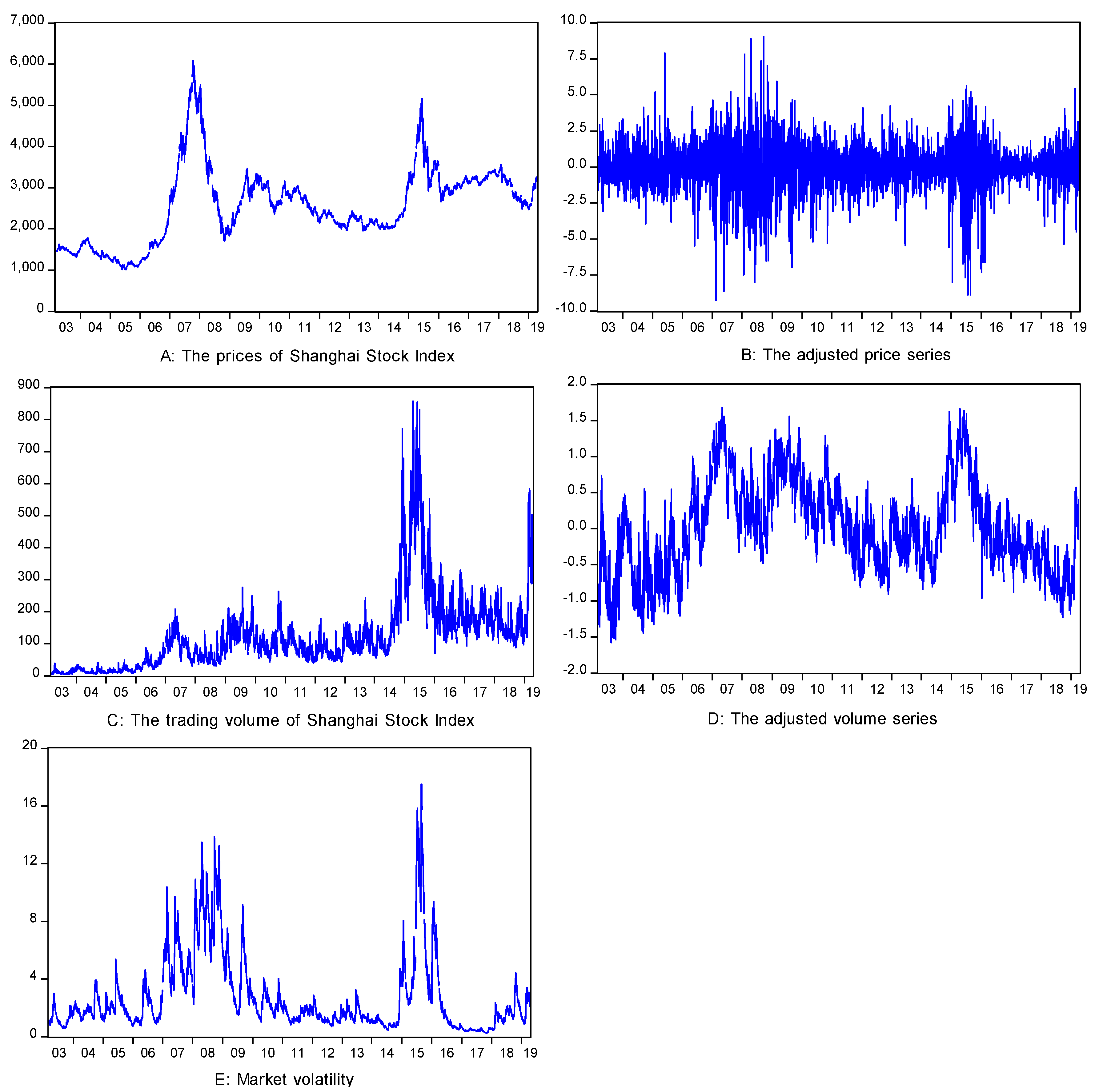
Figure 1. Data plots.
Sustainability 12 03322 g001
Figure 2. The selection process of time thresholds. (a) Setting one threshold value (b) setting two threshold values.
Sustainability 12 03322 g002
Figure 3. Four time-threshold value estimates.
Sustainability 12 03322 g003
Figure 4. The selection process of volatility thresholds. (a) Setting one threshold value (b) setting two threshold values.
Sustainability 12 03322 g004
Figure 5. Selection process of volatility thresholds (threshold variable: σ r e t , t 2 P ). (a) Setting one threshold value (b) setting two threshold values.
Sustainability 12 03322 g005
Figure 6. The selection process of volatility thresholds (threshold variable: σ r e t , t 2 C K ). (a) Setting one threshold value (b) setting two threshold values.
Sustainability 12 03322 g006
Table 1. Descriptive statistics.
VariableMeanMedianMaximumMinimumStd. Dev.SkewnessKurtosisJ-BADF
P t 2570.482574.686092.061011.50921.420.683.87428.28 ***
(0.0000)
−2.00
(0.2858)
Q t 121.9098.04857.134.08115.392.3710.4812,801.70 ***
(0.0000)
−3.60 *
(0.0058)
r e t t 0.020.069.03−9.261.60−0.507.423357.60 ***
(0.0000)
−61.42 ***
(0.0001)
vol t 0.00−0.041.69−1.580.630.222.4973.10 ***
(0.0000)
−4.9825 ***
(0.0000)
σ r e t , t 2 2.751.7817.520.252.652.107.646389.75 ***
(0.0000)
−4.2570 ***
(0.0005)
Note: p-value in parentheses. * and *** represent significance level at the 5% and 0.1%, respectively.
Table 2. Results for the Granger causality tests (full sample).
Null HypothesisAlternative Hypothesis χ 2   Statistic Test Result
Volume does not Granger cause price v o l t G . C r e t t 12.76 *
(0.0471)
Reject
Price does not Granger cause volume r e t t G . C v o l t 369.25 ***
(0.0000)
Reject
Note: X G . C Y denotes X Granger causes Y. p-value in parentheses. * and *** represent significance level at the 5% and 0.1%, respectively.
Table 3. The estimation results of time threshold values.
Threshold VariableSetting the Numberof Threshold ValuesThreshold Value EstimateLR Test
Equation RetEquation Vol
Panel A: sample period 2003/3/4–2019/4/22
t 1T = 2015/06/1188.56 ***
(0.0000)
321.76 ***
(0.0000)
t 2t1 = 2015/06/11
t2 = 2016/03/31
88.56 ***
(0.0000)
321.76 ***
(0.0000)
Panel B: sample period 2003/3/4–2015/06/11
t 1t’ =2007/10/1531.71 ***
(0.0000)
157.75 ***
(0.0000)
t 2t3 =2007/10/15
t4 =2008/11/03
31.71 ***
(0.0000)
157.75 ***
(0.0000)
Note: p-value in parentheses. *** represent significance level at the 0.1%, respectively.
Table 4. Results of the Granger-causality tests (subsamples).
Null HypothesisAlternative Hypothesis χ 2   Statistic Test Result
Subsample 1: 2003/3/4–2007/10/15
Volume does not Granger causes price v o l t G . C r e t t 16.88 **
(0.0020)
Reject
Price does not Granger causes volume r e t t G . C v o l t 94.95 ***
(0.0000)
Reject
Subsample 2: 2007/10/15–2008/11/03
Volume does not Granger causes price v o l t G . C r e t t 1.39
(0.2392)
Accept
Price does not Granger causes volume r e t t G . C v o l t 16.64 ***
(0.0000)
Reject
Subsample 3: 2008/11/03–2015/06/11
Volume does not Granger causes price v o l t G . C r e t t 14.83
(0.0625)
Accept
Price does not Granger causes volume r e t t G . C v o l t 309.81 ***
(0.0000)
Reject
Subsample 4: 2015/06/11–2016/03/31
Volume does not Granger causes price v o l t G . C r e t t 3.57
(0.0587)
Accept
Price does not Granger causes volume r e t t G . C v o l t 0.02
(0.8959)
Accept
Subsample 5: 2016/03/31–2019/4/22
Volume does not Granger causes price v o l t G . C r e t t 0.47
(0.9261)
Accept
Price does not Granger causes volume r e t t G . C v o l t 68.90 ***
(0.0000)
Reject
Note: X G . C Y denotes X Granger causes Y. p-value in parentheses. ** and *** represent significance level at the 1% and 0.1%, respectively.
Table 5. The estimation results of volatility thresholds.
Threshold VariableSetting the Numberof Threshold ValueThreshold EstimatesLR test
Equation retEquation vol
σ r e t , t 2 1 σ r e t , t 2 = 6.5261.58 ***
(0.0000)
115.32 ***
(0.0000)
σ r e t , t 2 2 σ r e t , t 1 2 = 3.09
σ r e t , t 2 2 = 6.52
61.58 ***
(0.0000)
115.32 ***
(0.0000)
Note: p-value in parentheses. *** represent significance level at the 0.1%, respectively.
Table 6. TVAR regression results (threshold variable: σ r e t , t 2 ).
Explanatory
Variable
(1)
σ r e t , t 2 6.52
(2)
σ r e t , t 2 3.09
(3)
3.09 < σ r e t , t 2 6.52
(4)
σ r e t , t 2 > 6.52
Equation retEquation volEquation retEquation volEquation retEquation volEquation retEquation vol
ret(-1)0.0088
(0.0197)
0.0433 ***
(0.0023)
0.0066
(0.0258)
0.0515 ***
(0.0030)
0.0122
(0.0310)
0.0328 ***
(0.0036)
0.0181
(0.0307)
0.0199 ***
(0.0036)
ret(-2)−0.0506 *
(0.0223)
0.0076 **
(0.0026)
−0.0316
(0.0297)
0.0075 *
(0.0034)
−0.0796 *
(0.0350)
0.0078
(0.0040)
−0.0370
(0.0280)
−0.0045
(0.0032)
ret(-3)0.0717 **
(0.0224)
0.0092 ***
(0.0026)
0.0427
(0.0294)
0.0068 *
(0.0034)
0.1286 ***
(0.0361)
0.0130 **
(0.0042)
−0.0719 **
(0.0274)
−0.0005
(0.0032)
ret(-4)−0.0102
(0.0225)
−0.0003
(0.0026)
−0.0026
(0.0293)
0.0029
(0.0034)
−0.0169
(0.0369)
−0.0052
(0.0043)
0.1051 ***
(0.0271)
0.0003
(0.0031)
ret(-5)0.0152
(0.0223)
−0.0013
(0.0026)
−0.0096
(0.0289)
0.0012
(0.0033)
0.0519
(0.0368)
−0.0028
(0.0043)
−0.0351
(0.0269)
−0.0028
(0.0031)
ret(-6)−0.0525 *
(0.0214)
−0.0083 ***
(0.0025)
−0.0551 *
(0.0278)
−0.0067 *
(0.0032)
−0.0370
(0.0350)
−0.0088 *
(0.0041)
−0.0919 ***
(0.0263)
−0.0050
(0.0031)
vol(-1)0.3953 **
(0.1522)
0.5873 ***
(0.0177)
0.3205
(0.1688)
0.5712 ***
(0.0195)
0.7927 *
(0.3695)
0.6383 ***
(0.0428)
−0.2316
(0.4221)
0.6234 ***
(0.0489)
vol(-2)0.0046
(0.1777)
0.1112 ***
(0.0206)
0.2036
(0.1946)
0.1338 ***
(0.0225)
−1.0370 *
(0.4515)
0.0108
(0.0523)
0.7211
(0.4611)
0.1568 **
(0.0535)
vol(-3)−0.1071
(0.1786)
0.0821 ***
(0.0207)
−0.1237
(0.1963)
0.0577 *
(0.0227)
0.1943
(0.4513)
0.2063 ***
(0.0522)
0.2895
(0.4541)
0.0267
(0.0527)
vol(-4)−0.1183
(0.1795)
0.0683 **
(0.0208)
−0.1965
(0.1963)
0.0732 **
(0.0227)
0.2009
(0.4632)
0.0085
(0.0536)
−0.6416
(0.4381)
0.0595
(0.0508)
vol(-5)0.0173
(0.1782)
0.0586 **
(0.0207)
0.1213
(0.1946)
0.0713 **
(0.0225)
−0.4300
(0.4637)
0.0150
(0.0537)
−0.5812
(0.4432)
−0.0035
(0.0514)
vol(-6)−0.0645
(0.1514)
0.0590 ***
(0.0176)
−0.2183
(0.1673)
0.0524 **
(0.0194)
0.5397
(0.3694)
0.0906 *
(0.0428)
0.4553
(0.3719)
0.0616
(0.0431)
Constant0.0508
(0.0272)
−0.0014
(0.0032)
0.0527
(0.0325)
−0.0047
(0.0038)
−0.0683
(0.0929)
0.0055
(0.0108)
−0.2337
(0.1246)
0.0222
(0.0145)
Note: The optimal lag order was determined to be 6 according to SIC criterion. Standard error in parenthesis, *, ** and *** represent significance level at the 5%, 1% and 0.1%, respectively.
Table 7. TVAR regression results (threshold variable: σ r e t , t 2 P ).
Explanatory
Variable
(1)
σ r e t , t 2 P 26.82
(2)
σ r e t , t 2 P 21.17
(3)
21.17 < σ r e t , t 2 P 26.82
(4)
σ r e t , t 2 P > 26.82
Equation retEquation volEquation retEquation volEquation retEquation volEquation retEquation vol
ret(-1)0.0256
(0.0272)
0.0560 ***
(0.0031)
0.0619
(0.0345)
0.0620 ***
(0.0040)
−0.0730
(0.0513)
0.0463 ***
(0.0059)
−0.0084
(0.0213)
0.0238 ***
(0.0024)
ret(-2)−0.0581 *
(0.0239)
0.0052
(0.0027)
−0.0813 **
(0.0290)
0.0034
(0.0033)
0.0152
(0.0514)
0.0076
(0.0059)
−0.0388
(0.0264)
0.0001
(0.0030)
ret(-3)0.0141
(0.0226)
0.0080 **
(0.0026)
0.0248
(0.0270)
0.0054
(0.0031)
0.0005
(0.0449)
0.0127 *
(0.0052)
0.0337
(0.0272)
0.0026
(0.0031)
ret(-4)−0.0120
(0.0218)
0.0034
(0.0025)
−0.0172
(0.0263)
0.0047
(0.0030)
0.0249
(0.0439)
−0.0026
(0.0051)
0.1187 ***
(0.0273)
−0.0028
(0.0031)
ret(-5)−0.0208
(0.0221)
0.0008
(0.0025)
−0.0374
(0.0259)
0.0002
(0.0030)
0.0484
(0.0469)
0.0006
(0.0054)
0.0176
(0.0265)
−0.0059
(0.0031)
ret(-6)−0.0580 **
(0.0200)
−0.0062 **
(0.0023)
−0.0753 **
(0.0236)
−0.0069 *
(0.0027)
−0.0069
(0.0422)
−0.0039
(0.0049)
−0.0668 *
(0.0279)
−0.007 *
(0.0032)
vol(-1)0.4183 *
(0.1780)
0.5676 ***
(0.0205)
0.2362
(0.2018)
0.5785 ***
(0.0232)
1.4935 **
(0.5189)
0.6000 ***
(0.0598)
−0.1141
(0.3237)
0.5889 ***
(0.0373)
vol(-2)0.0722
(0.1877)
0.1409 ***
(0.0216)
0.3307
(0.2048)
0.1466 ***
(0.0236)
−1.6279 **
(0.5322)
0.0512
(0.0613)
0.4568
(0.3652)
0.1277 **
(0.0421)
vol(-3)−0.1484
(0.1846)
0.0479 *
(0.0212)
−0.2420
(0.2003)
0.0439
(0.0231)
0.1456
(0.5121)
0.0779
(0.0590)
0.5060
(0.3854)
0.1595 ***
(0.0444)
vol(-4)−0.1196
(0.1792)
0.0733 ***
(0.0206)
−0.1397
(0.1969)
0.0570 *
(0.0227)
0.3506
(0.4612)
0.1513 **
(0.0531)
−0.5460
(0.4230)
0.0383
(0.0487)
vol(-5)−0.0393
(0.1801)
0.0509 *
(0.0207)
0.0402
(0.1958)
0.0720 **
(0.0226)
−0.3109
(0.4921)
−0.0764
(0.0567)
−0.5117
(0.4010)
0.0426
(0.0462)
vol(-6)−0.0546
(0.1548)
0.0814 ***
(0.0178)
−0.1211
(0.1685)
0.0669 ***
(0.0194)
0.2811
(0.4285)
0.1669 ***
(0.0494)
0.0437
(0.3277)
−0.0195
(0.0377)
Constant0.0321
(0.0288)
−0.0033
(0.0033)
0.0219
(0.0328)
0.0005
(0.0038)
−0.0165
(0.0947)
−0.0239 *
(0.0109)
0.1847
(0.1063)
0.0065
(0.0122)
Note: The optimal lag order was determined to be 6 according to SIC criterion. Standard error in parenthesis, *, ** and *** represent significance level at the 5%, 1% and 0.1%, respectively.
Table 8. TVAR regression results (threshold variable: σ r e t , t 2 C K ).
Explanatory
Variable
(1)
σ r e t , t 2 C K 30.78
(2)
σ r e t , t 2 C K 22.33
(3)
22.33 < σ r e t , t 2 C K 30.78
(4)
σ r e t , t 2 C K > 30.78
Equation retEquation volEquation retEquation volEquation retEquation volEquation retEquation vol
ret(-1)0.0497 *
(0.0223)
0.0501 ***
(0.0026)
0.0540
(0.0278)
0.0560 ***
(0.0032)
0.0107
(0.0389)
0.0362 ***
(0.0045)
−0.0628 *
(0.0261)
0.0143 ***
(0.0030)
ret(-2)−0.0730 **
(0.0225)
0.0025
(0.0026)
−0.0913 **
(0.0279)
0.0029
(0.0032)
−0.0809
(0.0417)
−0.0026
(0.0048)
−0.0047
(0.0293)
0.0020
(0.0034)
ret(-3)0.0424 *
(0.0211)
0.0066 **
(0.0024)
0.0324
(0.0254)
0.0083 **
(0.0029)
0.0645
(0.0394)
0.0013
(0.0045)
−0.0448
(0.0308)
0.0006
(0.0035)
ret(-4)−0.0092
(0.0206)
0.002
(0.0024)
−0.0213
(0.0250)
0.0027
(0.0029)
−0.0158
(0.0385)
−0.0031
(0.0044)
0.1648 ***
(0.0312)
−0.0053
(0.0036)
ret(-5)−0.0191
(0.0205)
−0.0012
(0.0024)
−0.0257
(0.0254)
−0.0005
(0.0029)
−0.0226
(0.0361)
−0.0046
(0.0042)
0.0224
(0.0306)
−0.0055
(0.0035)
ret(-6)−0.0579 **
(0.0195)
−0.0060 **
(0.0022)
−0.0752 ***
(0.0225)
-0.0070 **
(0.0026)
−0.0194
(0.0398)
−0.0034
(0.0046)
−0.0635 *
(0.0308)
−0.0105 **
(0.0035)
vol(-1)0.4115 *
(0.1649)
0.5956 ***
(0.0190)
0.3268
(0.1852)
0.5920 ***
(0.0213)
1.3405 **
(0.4545)
0.6616 ***
(0.0524)
0.1230
(0.3851)
0.5975 ***
(0.0444)
vol(-2)0.0647
(0.1795)
0.1285 ***
(0.0207)
0.2910
(0.1956)
0.1273 ***
(0.0225)
−1.2933 **
(0.4763)
0.1144 *
(0.0549)
0.3342
(0.4413)
0.0994
(0.0508)
vol(-3)−0.2174
(0.1776)
0.0541 **
(0.0205)
−0.2845
(0.1912)
0.0477 *
(0.0220)
0.2600
(0.4921)
0.0875
(0.0567)
0.6945
(0.4889)
0.1774 **
(0.0563)
vol(-4)−0.0445
(0.1740)
0.0731 ***
(0.0201)
−0.1192
(0.1900)
0.0626 **
(0.0219)
0.5712
(0.4480)
0.1502 **
(0.0516)
−0.8105
(0.5586)
−0.0274
(0.0643)
vol(-5)0.0043
(0.1743)
0.0486 *
(0.0201)
0.0401
(0.1887)
0.0667 **
(0.0217)
−0.2831
(0.4557)
−0.0505
(0.0525)
−1.0655 *
(0.5171)
0.0556
(0.0596)
vol(-6)−0.1127
(0.1485)
0.0666 ***
(0.0171)
−0.0800
(0.1612)
0.0706 ***
(0.0186)
−0.4978
(0.4066)
0.0260
(0.0468)
0.6897
(0.4241)
0.0420
(0.0488)
Constant0.0343
(0.0275)
0.0006
(0.0032)
0.0656 *
(0.0309)
0.0023
(0.0036)
−0.1636
(0.0986)
−0.0288 *
(0.0114)
−0.0169
(0.1444)
−0.0239
(0.0166)
Note: The optimal lag order was determined to be 6 according to SIC criterion. Standard error in parenthesis, *, ** and *** represent significance level at the 5%, 1% and 0.1%, respectively.