Carbon and Water Footprints of Tibet: Spatial Pattern and Trend Analysis

Abstract

Tibet in China has extremely a fragile natural ecosystem, which is under a great pressure from global changes. The carbon footprint (CF) and water footprint (WF), reflecting the pressures of regional development on the natural environment, represent a lacuna in the field of study in Tibet due to missing data. In this paper, the 2012 multi-regional input–output table of China was employed to quantify the CF and WF of Tibet and the relationship between Tibet and other provinces of China. Spatial pattern and key sectors were also studied to demonstrate the current characters and the future trend of footprints. Tibet’s carbon emission was 4.0 Mt, 32.7% of CF, indicating that Tibet was a net importing region of carbon emission. Tibet received embodied carbon emission by trade from other regions, especially from Hebei, Inner Mongolia and Henan provinces, but played a complex role in virtual water allocation by transferring to most provinces and receiving from some provinces. The CF of Tibet will increase under different scenarios of 2030, but the WF can be restricted to 2.5 Gt in the slow scenario. In the future, imports of virtual resources will benefit the fragile ecosystem of Tibet and moreover, it is vital to restrict the local resource-intensive sectors and improve resource-use efficiency.

1. Introduction

As a serious and urgent issue, climate change has attracted much attention around the world. The Intergovernmental Panel on Climate Change (IPCC) predicts that globally we need to reduce the release of anthropogenic greenhouse gas (GHG) emissions to ‘near zero’ by 2100, to be likely to limit global warming to 2 °C and prevent the worst effects of climate change [1]. The Paris Agreement strengthened the mitigation ambition to keep further warming to 1.5 °C below pre-industrial levels [2]. Policies have been designed in response to this challenge in developed and developing countries by controlling and reducing direct carbon emissions, for which scholars have also suggested to control the carbon footprints of countries and people. On the other hand, as the distribution of water resources is very sensitive to climate change, direct water consumption and the water footprint of regions is another key issue in climate change adaptation. More strikingly, a new concept, the energy–food–water–climate nexus, was proposed to reveal the operation mechanism of the complex system, so as to adapt and mitigate climate change [3]. China and its provinces have been analyzed in-depth because of their great and fast-growing carbon emissions and water consumption. However, one region in China has hardly been included in such studies and lacks any footprint assessment to the authors’ knowledge. That is the administrative region of Tibet, a special region on the world’s largest and highest Plateau and China’s second largest provincial-level administrative region with an area of 1.22 million km². With rich water resources and hydropower resources, as well as with an extremely fragile natural ecosystem, Tibet is a crucial region in response to climate change. Assessing the carbon and water footprint of Tibet and exploring their characteristics will support climate change mitigation and adaptation in Tibet and the regions around it.

In recent years, studies on reducing carbon emissions and solving water shortage have been springing up, not only at the global level [4], national level [5], but also at the regional [6], urban [7], family and individual levels [8]. Consumption-based (CB) accounting perspectives have emerged alongside the traditional production-based frameworks, enabling GHG emissions responsibility to be allocated to the final consumer [9]. The former perspective has the added benefit of capturing emissions embodied in goods and internationally traded products [10]. This allows for the GHG emissions from human consumption, which is ultimately the driver of anthropogenic climate change, to be understood and for effective mitigation policy to be designed [11]. The concept of a carbon footprint and water footprint were both inspired by the ecological footprint. Carbon footprint is defined as the total set of greenhouse gas emissions caused by an organization, event, product or person [12]. Water footprint refers to the amount of water needed for all the products and services that human beings consume to survive [13]. The input–output (IO) analysis is one of the main methods for implementing the CB footprint. Many studies have applied the single-regional input–output method to estimate the footprints [14] based on the assumption that the same products will be produced in the same sector by using the same domestic technology. The results carry great errors because of the different technologies in different countries and regions, which supply products to the studied region through international or domestic supply chains. The multi-regional input–output (MRIO) model is widely used in the research of carbon footprint (CF) and water footprint (WF) [15], with a comprehensive system boundary to avoid the errors of an incomplete supply chain. Moreover, regional relationships can be evaluated by the inter-regional flows, as the spatial pattern of footprint distribution. In terms of CF research, MRIO analysis can be used to calculate the intensity and footprints, as well as the net emissions flow between countries [16]. Similar studies taking China [17] and its cities [18] as study areas demonstrated the diversity in the country. In terms of WF research, Cai et al. incorporated the blue WF, related with the water quantity and the grey WF, related with water quality, into the virtual water flow analysis based on the MRIO model of 2007 [19]. Water scarcity was a concern for some scholars when assessing the WF and the embedded or virtual water flows in inter-regional trade [20]. Many studies have shown that the direct water consumption intensity and consumption levels are the dominant driver factors of a WF [21]. Recent studies have extended the MRIO model to broader issues, such as the analysis of household cross-border carbon emissions [22] or the agricultural water footprint [23].

With the rapid development of China’s economy, residents’ consumption, as well as its indirect emissions also increase gradually [24]. The uneven spatial distribution of resources and the mismatch between economic development and other major production factors, result in the separation of the production and consumption of water-intensive products [19]. In recent years, there have been a lot of studies on the CF [25] and WF [26] of Chinese provinces, while the location and inequality of the footprint is of significance [15].

Most previous studies have researched the trade of a single resource or emission, but the interaction between two types of virtual resource trade is a lacuna in the study [27]. To date, there has been little analysis to expand the cognition of the resource footprint of Tibet, due to the insufficient statistical data on Tibet [28]. In 2015, the IO table of the Tibet Autonomous Region was constructed and published for the first time, thus Tibet can be inserted into China’s multi-regional input–output (MRIO) table of 2012.

Based on the MRIO table in 2012, this paper evaluated the CF and WF of the Tibet Autonomous Region, as well as the embodied carbon emissions and virtual water trade between Tibet and other regions according to a classic scheme. The key industrial sectors of CF and WF, as well as the key regional trading partners, were identified to reveal the characteristics of Tibet. After that, the CF and WF of Tibet in future scenarios were forecasted based on a trend analysis of coefficients and economic development, so that effective suggestions and countermeasures can be proposed to realize strict resource control in the future. This paper, for the first time for all we know, compared Tibet with other provinces in the perspective of CF and WF, and revealed relationships between Tibet and other provinces by embodied carbon emissions and virtual water trade. In addition, a scenario analysis was employed to connect present and future of Tibet’s CF and WF, and explore the effects of efficiency improvement. After all, the future trends of CF and WF is much more significant than the past situation when proposing policy suggestions for sustainable development.

2. Materials and Methods

2.1. Method to Estimate Regional Footprints

The MRIO model has been widely used in the study of CF and WF and inter-regional trade. In order to calculate the embodied carbon and virtual water flows among the provinces of China, we used a MRIO table with carbon and water accounting in this study. As introduced in other literatures, in a MRIO table with m regions and n sectors, there is an equation and its transformation, as shown in Equations (1) and (2):

X = AX + F

(1)

X = (I − A)⁻¹F

(2)

where I is the identity matrix, X is the total output matrix, A is the direct consumption coefficient matrix and F is the final demand matrix. (I − A)⁻¹ represents the Leontief inverse matrix under the IO model [4].

In order to calculate the CF and WF, the carbon emissions coefficient and the direct water consumption coefficient of the sector must be calculated first. They can be written as vectors.

$$E^r=[e_j^r],e_j^r=c_j^r/x_j^r$$

(3)

$$Q^r=[q_j^r],q_j^r=w_j^r/x_j^r$$

(4)

where $E^r$ is the carbon emissions coefficient of region r, $e_j^r$ is the carbon emissions coefficient of sector j in region r, $c_j^r$ is the carbon emissions of sector j in region r, $x_j^r$ is the total output of sector j in region r, $Q^r$ is the direct water consumption coefficient of region r, $q_j^r$ is the direct water consumption of sector j in region r and $w_j^r$ is the direct water consumption of sector j in region r.

We established a method to estimate the regional CF and WF and the inter-regional flows based on two literatures [10,17]. $C^{rs}$ is the embodied carbon emissions transferred from region r to region s and $W^{rs}$ is the virtual water transferred from region r to region s, which can be calculated by Equations (5) and (6):

$$C^{rs}=\underset{m\mathrm{regions}}{\underbracket{\left[0,\dots e_1^r,\dots e_n^r,\dots 0\right]}}{\left(I-A\right)}^{-1}{F}^s$$

(5)

$$W^{rs}=\underset{m\mathrm{regions}}{\underbracket{\left[0,\dots q_1^r,\dots q_n^r,\dots 0\right]}}{(I-A)}^{-1}{F}^s$$

(6)

$F^s$ is the final demand vector of region s. $\left[0,\dots e_1^r,\dots e_n^r,\dots 0\right]$ is a vector of carbon emissions coefficients of m regions with all elements set as 0 except those in region r. Therefore, $C^{rs}$ is the carbon emissions in region r because of the final demand in region s, that is, the embodied carbon emissions transferred from region r to region s. The same goes for the $W^{rs}$.

The net amount of the embodied carbon emissions and virtual water transferred from region s to region r can be calculated by Equations (7) and (8):

$$C_{net}^{sr}=C^{sr}-C^{rs}$$

(7)

$$W_{net}^{sr}=W^{sr}-W^{rs}$$

(8)

The CF of region r consists of the following four parts—the household direct part $C_h^r$, the local emission caused by local final demand $C^{rr}$, the net part embodied in domestic trade with all other regions ${\displaystyle \sum }_{\mathrm{s}=1,\mathrm{r}\ne \mathrm{s}}^{\mathrm{m}}{C}^{sr}$ and the net part embodied in international trade $∆C_{im}$. The same goes for the WF.

$$C{F}^r=C_h^r+C^{rr}+{\displaystyle \sum }_{\mathrm{s}=1,\mathrm{r}\ne \mathrm{s}}^{\mathrm{m}}{C}^{sr}+∆C_{im}$$

(9)

$$W{F}^r=W_h^r+W^{rr}+{\displaystyle \sum }_{\mathrm{s}=1,\mathrm{r}\ne \mathrm{s}}^{\mathrm{m}}{W}^{sr}+∆W_{im}$$

(10)

2.2. Method to Predict Regional Footprints

A large uncertainty existed in the regional CF and WF forecasting for the next decades, as they were determined by the change of final demand, industrial structure and supply chain, production technology and resource efficiencies, according to the estimation method. However, most of them were lacking a basis for the prediction in a developing region. As the growth of final demand and resource efficiencies are the most important variables in footprints, this study focused on two important variables associated with footprints, the changes in final demand and the coefficients of industrial sectors. The former was forecasted according to the previous growth rate of the GDP, assuming that the growth rate of final demand was equal to that of the GDP in Tibet. The latter was forecasted according to national and regional plans, including local coefficients of the region as well as endemic ones.

We took the regional CF prediction as an example. The relationship between the regional carbon emission and CF could be clarified. The regional carbon emission consisted of four parts—local household emission, local emission caused by local final demand, by final demand of all other regions and by other countries, as shown in Equation (11):

$$CE=C_h^r+C^{rr}+{\displaystyle \sum }_{\mathrm{s}=1,\mathrm{r}\ne \mathrm{s}}^{\mathrm{m}}{C}^{rs}+∆C_{ex}$$

(11)

As a semi-closed economy with very limited international trade, Tibet’s $∆C_{im}$ and $∆C_{ex}$ are very limited and could be ignored. Therefore, Equation (9) can be transformed into Equation (12):

$$C{F}^r=\left(C_h^r+C^{rr}\right)+{\displaystyle \sum }_{\mathrm{s}=1,\mathrm{r}\ne \mathrm{s}}^{\mathrm{m}}{C}^{sr}=C{E}^r-{\displaystyle \sum }_{\mathrm{s}=1,\mathrm{r}\ne \mathrm{s}}^{\mathrm{m}}{C}^{rs}+{\displaystyle \sum }_{\mathrm{s}=1,\mathrm{r}\ne \mathrm{s}}^{\mathrm{m}}{C}^{sr}$$

(12)

The CF can be calculated based on regional carbon emissions and net carbon flows. We assumed the local final demand and that the exports and imports of region r was growing in correlation with the GDP of the region r, which was defined as multi-aspect simultaneous growth. Local emissions will follow the change of local emission coefficients and emission import will follow the change of emission coefficients in other regions. Both of them will follow the change of the GDP of the region r. The CF in the year of t1 can be calculated based on multi-change rates as shown in Equation (13):

$$\begin{array}{c}C{F}_{t1}^r=C{E}_{t1}^r-{\displaystyle {\displaystyle \sum }_{\mathrm{s}=1,\mathrm{r}\ne \mathrm{s}}^{\mathrm{m}}}{C}_{t1}^{rs}+{\displaystyle {\displaystyle \sum }_{\mathrm{s}=1,\mathrm{r}\ne \mathrm{s}}^{\mathrm{m}}}{C}_{t1}^{sr}\approx \\ [(C{E}_{t0}^r-{\displaystyle {\displaystyle \sum }_{\mathrm{s}=1,\mathrm{r}\ne \mathrm{s}}^{\mathrm{m}}}{C}_{t0}^{rs})\left(1-p_r\right)+{\displaystyle {\displaystyle \sum }_{\mathrm{s}=1,\mathrm{r}\ne \mathrm{s}}^{\mathrm{m}}}{C}_{t0}^{sr}\left(1-q_s\right)]\left(1+g_r\right)\end{array}$$

(13)

where CF_t1 is the CF of Tibet in year t1, CE_t0 is the carbon emissions of Tibet in in year t0, $p_r$ is the reduction rate of carbon emissions per unit of GDP of the region r from year t0 to t1, $q_s$ is the reduction rate of carbon emissions per unit of GDP of the region s from year t0 to t1 and $g_r$ is the growth rate of the GDP of the region r from year t0 to t1. According to the method, we can calculate the CF and WF of Tibet from 2012–2030 if all of the change rates are available.

As uncertainty existed in the prediction, two scenarios were built to reflect the upper and lower limits of the prediction, which were a scenario with a high growth rate (SH) and a scenario with a low growth rate (SL). Therefore, there were two simple scenarios investigating to explore the possible ranges of regional CF and WF in the future.

2.3. Data Sources

In this study, three types of data were used: (1) basic economic and geographic data, (2) China’s MRIO table in 2012 and (3) the carbon emissions and water consumptions for each sector of each region in China. The basic economic and geographic data were from the Statistical Yearbook of Tibet [29]. China’s MRIO table in 2012 was compiled by the Institute of Geographic Sciences and Natural Resources, Chinese Academy of Sciences [30]. This MRIO table was the latest edition for China at the time, which included 31 provinces, with 30 sectors in each province. The 30 sectors are shown in

Table 1. Sector classification.

Code	Sector	Code	Sector	Code	Sector
S1	Agriculture	S11	Petroleum refining coking and nuclear fuel	S21	Other manufacturing
S2	Coal mining and processing	S12	Chemical industry	S22	Electricity and hot water production and supply
S3	Crude petroleum and natural gas	S13	Non-metallic mineral products	S23	Gas and water production and supply
S4	Metal ore mining	S14	Metal smelting and processing	S24	Construction
S5	Non-metallic minerals and other mining	S15	Metal products	S25	Transportation and warehousing
S6	Food processing and tobaccos	S16	General and specialist machinery	S26	Wholesale and retailing
S7	Textile	S17	Transport equipment	S27	Hotel and restaurant
S8	Clothing, leather, fur, etc.	S18	Electrical equipment	S28	Leasing and commercial services
S9	Wood processing and furnishing	S19	Electronic equipment	S29	Scientific research
S10	Paper making, printing, stationery, etc.	S20	Instrument and meter	S30	Other services

.

The carbon emission of each sector and each province in China was obtained from the China Emission Accounts and Datasets [31], while Tibet’s direct carbon emission was from previous literature [32]. For the water consumption data of various sectors in China, that of agriculture sector was from China Statistical Yearbook [33], while that of the other sectors were from the China Statistical Yearbook on Environment [34]. The data on water consumption in Tibet and other provinces were from the National Data on the website of the National Bureau of Statistics of China [35]. The carbon emission and water consumption in each sector of each province were estimated based on these data and the method proposed by the literature [36].

3. Results and Policy Implications

3.1. Carbon Emissions and Water Consumption

The Tibet Autonomous Region (or Tibet) is located on China’s southwest region and covers a total area of 1,228,400 km², making it the second largest province in China. The location of Tibet in China is illustrated in Figure 1. The area with an elevation of above 4000 m accounts for 85.1% of the total area of the whole region, and Tibet has the highest altitude in the world, and is known as the “Roof of the World” and “the Third Pole of the Earth”. The weather in Tibet is characterized by less precipitation, seasonality, high night rain rate, and the annual precipitation ranges from 66.3 to 894.5 mm, showing a decreasing distribution pattern from southeast to northwest. The annual precipitation is highly concentrated from May to September. Tibet is rich in water resources and has a large area of water. Surface water includes rivers, lakes, swamps, glaciers and other forms, of which rivers and lakes are the most important part. Tibet has 28 rivers with a drainage area of more than 10,000 km², with a total water resource of 439,465 billion m³ (excluding groundwater), ranking first in China, as well as for acreage of water and water resources per capita [37].

In 2018, Tibet maintained a population of 3.44 million and urbanization rate of 31.1%. The GDP was 147.8 billion CNY (22.5 billion USD) and the GDP per capita was 43,800 CNY (6558 USD). The value-added of agriculture was 13.0 billion CNY, while construction was 51.4 billion CNY, service was 71.9 billion CNY. However, manufacturing was very limited, the value-added of which was only 11.5 billion CNY in 2018 [38].

Under the context of the increasing carbon emissions of China in recent years, Tibet’s carbon emission increased from 1.3 Mt CO₂ to 5.5 Mt CO₂ during 2003–2014 period, as shown in Figure 2. The carbon emission includes direct emission from transport and residential energy use. In the assessment of each province’s emission intensity (CO₂ emissions per GDP) reduction by the National Development and Reform Commission of China (2015), Tibet had the worst performance among China’s 31 provinces. It is urgent to reduce the carbon emissions intensity.

Water consumption was relatively stable during the 2004–2014 period, increasing from 2.80 Gt in 2004 to 3.05 Gt in 2014. In recent years, the water consumption in Tibet has been in a gradually decreasing process, mainly because of the decrease in the water-use intensity of irrigation and industrial systems, which has largely offset the increase in water demand caused by economic and social development. In addition, the improvement of people’s awareness of water conservation may have also played an important role. In the study year 2012, Tibet’s total water consumption was 2.98 Gt, while agriculture and industry consumed 2.71 Gt, 0.165 Gt respectively, and the service sector and residents consumed 0.104 Gt. Water consumption per capita was 976 t, which reached a peak in 2008 with 1315 t, and kept decreasing after that. Using water reasonably will benefit Tibet and China.

3.2. Carbon and Water Footprints

The CF and WF of 31 provinces were calculated based on the method in Section 2.1, and the CF and WF of Tibet were analyzed in detail. Tibet’s CF was 12.2 Mt CO₂ in 2012, much higher than the direct carbon emissions, 4.4 Mt CO₂. The WF of Tibet was 2.63 Gt in 2012, lower than Tibet’s water consumption, 2.98 Gt.

Figure 3 shows the per capita CF and per capita WF of the 31 provinces in 2012. Tibet had the smallest per capita CF with a value of 4.0 t, far less than the national average (8.0 t). Inner Mongolia and Ningxia had the highest per capita CF, with 24.4 t and 22.3 t respectively, which was 5–6 times higher than that of Tibet.

However, the per capita WF of Tibet reached 956.8 t, which was significantly higher than the national average (424.7 t). The per capita CF of Tianjin, Shanxi, Shanghai, Xinjiang and Liaoning exceeded 11.0 t with high levels. The provinces with the highest per capita WF were Xinjiang, Ningxia, Tibet and Heilongjiang, all of which were more than 800 t. Meanwhile, we found that Xinjiang, Inner Mongolia and Ningxia had high per capita CF and WF. Tibet was marked for low per capita CF and high per capita WF, compared with its neighboring regions.

The CF and WF of Tibet are divided by sector and shown in

Table 2. CF and WF of Tibet by sector. Sectors with a CF less than 1 kt and a WF less than 1 Mt are not listed. The CF and the WF of residents and the other services cannot be divided based on current the data and method, which does not affect the results.

Ranking	Sector	Carbon Footprint (kt)	Sector	Water Footprint (Mt)
1	Construction	8118	Agriculture	1738
3	Residents and other services	2721	Construction	368
4	Transportation and warehousing	341	Residents and other services	170
5	Wholesale and retailing	233	Food processing and tobaccos	148
6	Agriculture	201	Hotel and restaurant	56
7	Electricity and hot water production and supply	143	Chemical industry	20
8	Food processing and tobaccos	100	Wholesale and retailing	15
9	Non-metallic mineral products	98	Transportation and warehousing	15
10	Hotel and restaurant	91	Paper making, printing, stationery, etc.	9
11	Scientific research	46	Textile	8
12	Leasing and commercial services	34	Wood processing and furnishing	5
13	Metal ore mining	28	Scientific research	4
14	Paper making, printing, stationery, etc.	25	Metal ore mining	4
15	Chemical industry	14	Non-metallic mineral products	3
16	Metal products	9	Electricity and hot water production and supply	2
17	Textile	8	Clothing, leather, fur, etc.	2
18	Wood processing and furnishing	6	Leasing and commercial services	1
19	Clothing, leather, fur, etc.	4
20	Gas and water production and supply	3
	Total	12,224	Total	2568

. Construction and other services were prominent sectors of CF, with 8.1 Mt and 2.7 Mt CO₂, respectively, accounting for 66.4% and 22.3% of the total CF. The WF was mainly from the final demand of agriculture, construction, other services, food processing and tobaccos and hotels and restaurants. The WF of agriculture was 1.7 Gt, accounting for 64.6% of the total WF. Sectors of construction, agriculture and other services were prominent both in CF and WF. Tourism was the pillar industry of Tibet, which received 33.7 million tourists in 2018 and the total tourism revenue was 49 billion CNY. Therefore, tourism was the prominent part of the other services.

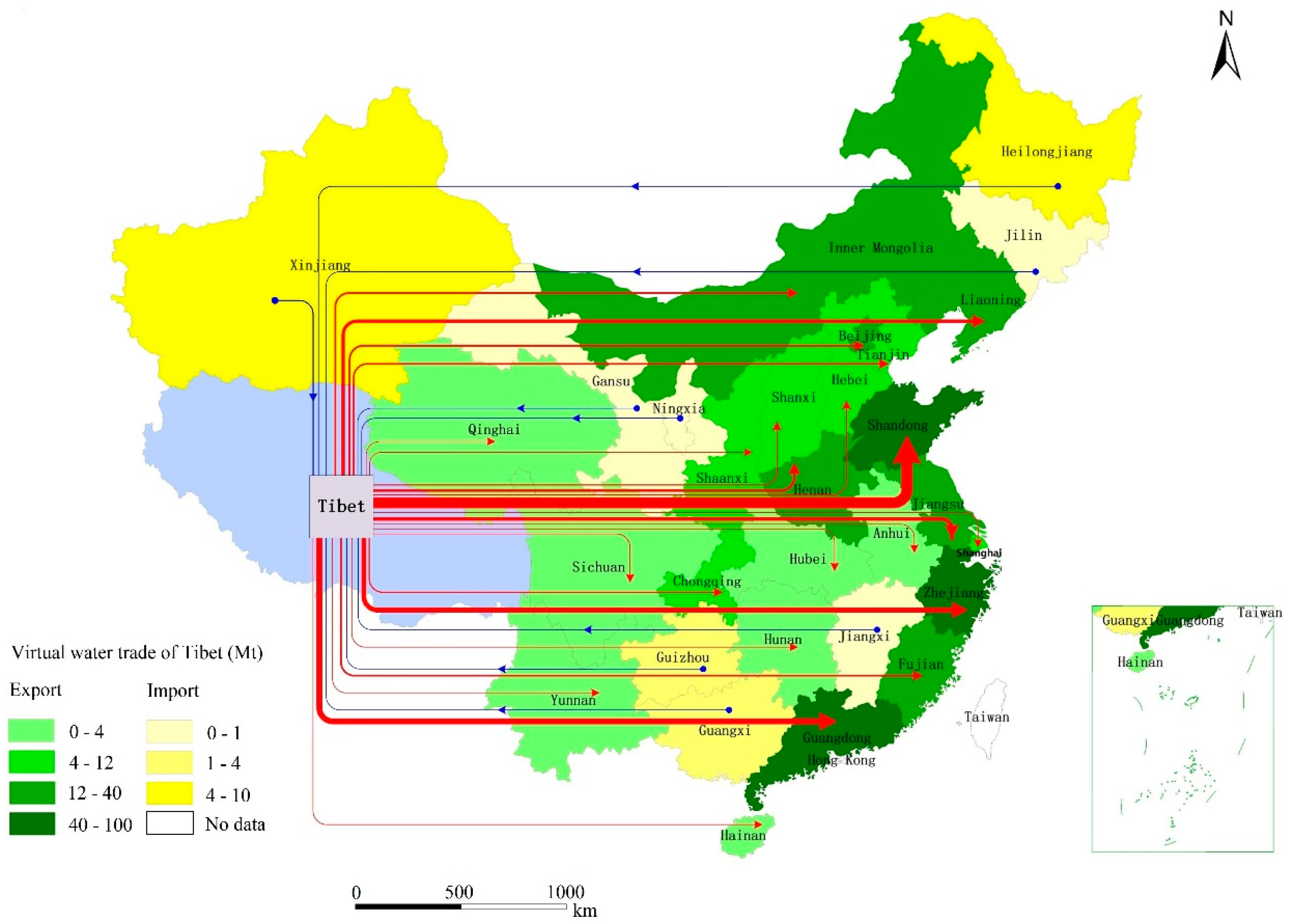
3.3. Domestic Trade of Embodied Carbon Emissions and Virtual Water

The inflow and outflow of embodied carbon emissions and virtual water generated by the commodity trade between Tibet and the other provinces were calculated. The net flows of virtual water or embodied carbon emissions were the inflow minus the outflow. The total amount of embodied carbon emissions transferred to Tibet reached 7.8 Mt in 2012. According to Figure 4, Tibet received the transfer of carbon from the 30 other provinces in China and 41.0% of the carbon inflows were from Hebei (10.0%), Inner Mongolia (9.2%), Henan (9.2%), Liaoning (6.7%) and Shandong (5.9%) provinces. Such pattern was mainly related to the economic structure of these provinces. Hebei had a solid industrial base with a huge iron and steel production. Henan and Shandong were the major economic provinces in China with strong and competitive industrial bases. These provinces were well developed in industries with high carbon emissions.

The total amount of virtual water transferred from Tibet to other provinces reached 355.1 Mt. As shown in Figure 5, Tibet played a complex role in virtual water allocation because it transferred the virtual water to most provinces and received virtual water from some provinces. Specifically, 62.4% of the total net virtual water outflow was from Shandong (27.4%), Guangdong (14.3%), Zhejiang (11.7%) and Jiangsu (9.0%) provinces. These provinces are located in coastal areas, with good economic development status and large populations.

We learned that Tibet was the main source of CF and the main destination of WF. All of the Tibet’s trading partners could be divided into four types according to the trading relationships and characteristics: carbon–water complementation, carbon sources, water destination and weak ties in carbon and water, as shown in

Table 3. Four types of relationships between Tibet and the other provinces.

	Large Water Flow	Small Water Flow
Large Carbon Flow	Type 1: Carbon–water complementation Provinces: Liaoning, Inner Mongolia, Henan, Shandong, Guangdong, Jiangsu	Type 2: Carbon sources Provinces: Hebei, Jilin, Shanxi, Anhui
Small Carbon Flow	Type 3: Water destination Provinces: Tianjin, Beijing, Zhejiang, Fujian	Type 4: Weak ties in carbon and water trade Provinces: Qinghai, Ningxia, Gansu, Heilongjiang, Xinjiang, Shaanxi, Shanghai, Hubei, Sichuan, Chongqing, Jiangxi, Hunan, Guizhou, Yunnan, Guangxi, Hainan

. There were large carbon and water flows between Tibet and a series of provinces, such as Liaoning, Inner Mongolia, Henan, Shandong, Guangdong and Jiangsu, which were the most prominent in the final products trade with Tibet. Tianjin, Beijing, Zhejiang, Fujian were destinations of water flows from Tibet, while Hebei, Jilin, Shanxi, Anhui were sources of carbon flows to Tibet. Different types provided the degree of importance of the trading partners to Tibet. Promoting trade between Tibet and one of the types will result in certain change. On the other hand, the CF and WF regulation will influence the trade pattern.

3.4. Scenario Analysis

Based on the calculation results of Tibet’s CF and WF in 2012, the future CF and WF of Tibet were determined according to the growth of GDP and the change of water consumption coefficient and carbon emissions coefficient per unit of GDP. Based on the constant price of China in 2012, two scenarios of GDP growth in Tibet were assumed: the scenario with a high growth rate (SH) and the scenario with a low growth rate (SL). The results are shown in Figure 6. In the scenario of SH, the economy of Tibet continues to grow steadily while the GDP growth rate in each “Five-Year Plan” decreases slightly and the forecast of Tibet’s GDP will reach 352.2 billion CNY in 2030. In the scenario of SL, the economic growth rate in Tibet slows down significantly, and the forecast of Tibet’s GDP will reach 291.2 billion CNY.

The changes of water consumption coefficient and carbon emissions coefficient of each province per unit of GDP are shown in

Table 4. Targets of carbon and water intensities. ① is from the 13th Five-Year Plan for National Economic and Social Development of Tibet. ② is from the 13th Five-Year Plan for National Economic and Social Development of the People Republic of China. ③ is from the 13th Five-Year Plan for controlling greenhouse gas emissions. ④ is from the 13th Five-Year Plan for building a water-conserving society.

Period	Carbon Intensity		Water Intensity
	Tibet	China	Tibet	China
2012–2015	−6.1% ①	−10.6% ②	−22.8% ①	−20.0% ④
2016–2020e	−12.0% ③	−18.0% ③	−35.0% ①	−23.0% ④
2021–2025e	−12.0%	−18.0%	−30.0%	−20.0%
2026–2030e	−12.0%	−18.0%	−25.0%	−20.0%

. From this, we could see that the reduction value of water consumption coefficient per unit of GDP in Tibet was significantly higher than the national average level. On the contrary, the reduction in carbon emissions coefficient was significantly lower than the national average level. Based on the relevant data about the 13th “Five-Year Plan” of Tibet and the national data, we forecast the changes of the water consumption coefficient and carbon emissions coefficient per unit of GDP in Tibet and China during the 2020–2030 period. According to the data in

Table 5. Forecast of carbon and water intensities. The calculation is based on the constant price of China in 2012.

Year	Carbon Intensity (t/103CNY)		Water Intensity (t/103CNY)
	Tibet	China	Tibet	China
2012	0.063	0.166	42.52	10.43
2015	0.059	0.149	32.84	8.35
2020e	0.052	0.122	21.34	6.43
2025e	0.046	0.100	14.94	5.14
2030e	0.040	0.082	11.21	4.11

and the actual carbon emissions and water consumption in 2012, we could get the water consumption coefficient and carbon emissions coefficient of per unit of GDP during the 2015–2030 period.

The forecast results of the CF and WF are shown in

Table 6. Forecast of Tibet’s CF and WF.

		2012	2015	2020		2025		2030
				SH	SL	SH	SL	SH	SH
Carbon (Mt)	Direct emissions	4.43	5.73	8.13	7.91	11.01	10.00	14.24	11.77
	Net inflow	7.80	9.45	12.37	12.04	15.47	14.04	18.48	15.28
	Footprint	12.23	15.18	20.50	19.95	26.48	24.04	32.72	27.05
Water (Gt)	Direct consumption	2.99	3.08	2.93	2.85	3.16	2.87	3.48	2.88
	Net inflow	−0.36	−0.38	−0.39	−0.38	−0.42	−0.38	−0.46	−0.38
	Footprint	2.63	2.70	2.54	2.47	2.74	2.49	3.02	2.50

. Under both scenarios, Tibet’s CF will increase year by year. The CF was predicted to reach 32.72 Mt in 2030 in SH scenario, which is about 1.2 times that of the SL scenario and 2.7 times that of what it was in 2012. It could be found that Tibet’s carbon emissions accounted for an increasing proportion in CF, because carbon intensity in other regions reduced faster than that in Tibet.

The WF was stable in the future. In the SL scenario, the WF of Tibet would be stable at 2.5 Gt. In the SH scenario, Tibet’s WF was still growing at a low rate and would reach 3.02 Gt by 2030. Although the economic growth would lead to an increase in the WF, the decrease in water consumption coefficient would help offset this increase, especially of that in agriculture. In addition, Tibet would be very likely to continue to export virtual water by inter-regional trade.

3.5. Policy Implications

Although there is still uncertainty in the estimation and prediction due to the limited statistical data, this study may have some new findings. Tibet is an import-dependent economy and its external carbon footprint accounts for 67.3% of the total carbon footprint, mainly reflected in construction and the other services industry. Although Tibet’s CF is low, its CF intensity, or CF per unit of GDP needs to be reduced, especially in the construction industry. Tibet’s water efficiency is also very low, especially of that in agriculture. Agriculture in Tibet has only just reached a certain level, as it is difficult to make quick growth. The WF will be reduced if the water efficiency of agriculture is improved. Tibet’s manufacturing industry is undeveloped and there is no plan to make a rapid development, so its direct emissions can be controlled. However, the consumption and investment by residents and companies will promote WF in the future, especially infrastructure construction, which contributes to capital formation and local development and is an important carrier of Tibet’s CF and WF, and also is a driving force for further growth. Tourism is a pillar industry in Tibet. Tourists and tourism income in Tibet will increase further with the increase of China’s per capita income, which is likely to promote Tibet’s CF and WF. As a result, the tourism service and hotel service have great potential in water and energy saving and carbon emission abatement.

For Tibet, how to balance the need of rapid economic development and emissions reduction has become particularly important. Based on the research results of this paper and considering the actual situation faced by Tibet and China, possible measures could be taken as follows. First, the local government can make policies with low-carbon purposes, for example, increasing the proportion of power from renewable energy, promoting clean transition in the production process, importing products from low-carbon regions. Second, Tibet should promote energy conservation and improve energy efficiency by introducing advanced technologies. Tibet’s CF is mainly from construction and services, which can be traced back to cement and transport, so it is significant to introduce cleaner production technologies and new energy vehicles. Third, Tibet needs to make full use of its resource advantages, such as waterpower resources and solar energy. Therefore, Tibet is likely to play a role in power export, alleviating power shortages and reducing energy consumption, so that it makes its own contribution to the national carbon emissions reduction.

4. Conclusions

Previous studies on China’s national and provincial footprints have generally ignored Tibet before Tibet was involved in China’s 2012 MRIO table. This study applied the IO model to calculate the CF and WF of 31 provinces in China, especially Tibet, and analyzed the trade flows of carbon and water between Tibet and other provinces in detail. This study has achieved the following main findings.

In 2012, Tibet’s CF was 12.2 Mt CO₂, with a net import carbon emissions of 7.8 Mt CO₂ (an import of 8.2 Mt CO₂ and an export of 0.4Mt CO₂). The WF of Tibet was 2.57 Gt in 2012, with a net outflow of 0.36 Gt (an import of 0.21 Gt and an export of 0.57 Gt). Construction, residents and other services in Tibet accounted for 66.4% and 22.3% of the total CF, respectively, while agriculture and construction accounted for 64.6% and 14.3% of the total WF, respectively. These are key sectors in which to realize low-carbon and water-saving targets for Tibet.

Tibet has received the embodied carbon from other 30 provinces in China, especially from Hebei, Inner Mongolia and Henan. Meanwhile, Tibet has taken on a complex role in virtual water allocation by exporting virtual water to most provinces and importing virtual water from some provinces. Among them, Shandong, Guangdong and Zhejiang province are the main provinces of virtual water destination.

Under the scenarios of SH and SL, the future CF of Tibet shows a growing trend, and will reach 32.72 Mt CO₂ in 2030, about 2.2–2.7 times of that in 2012. The WF will be stable at around 2.5 Gt under the SL scenario, but reach 3.02 Gt in 2030 under the SH scenario.

There are some limitations in this study. We only got the results of 2012, lacking the possibility of comparison with different years as the data are unavailable. The international import and export volume of Tibet is ignored in this study because of its relatively small value. There is a large gap between urban and rural regions in Tibet. For different cities, the CF and WF and the trade relationship with the outside are different, which cannot be studied with no data. The trade relationship between Tibet and the outside is restricted by traffic conditions, and the influence of future traffic conditions was not considered in the scenario analysis.

Future research will be implemented, such as a multi-year comparative study, the impact of the WF change on water resources in Tibet, the impact of various factors on the CF and WF, and carbon and water nexus.

References

1. Intergovernmental Panel on Climate Change. AR5 Climate Change 2014: Mitigation of Climate Change. Available online: https://www.ipcc.ch/report/ar5/wg3/ (accessed on 7 September 2019).
2. The United Nations Framework Convention on Climate Change. The Paris Agreement. Available online: https://unfccc.int/process-and-meetings/the-paris-agreement/the-paris-agreement/ (accessed on 7 September 2019).
3. Hoekstra, A.Y.; Chapagain, A.K. Water footprints of nations: Water use by people as a function of their consumption pattern. Water Resour. Manag. 2007, 21, 35–48. [Google Scholar] [CrossRef]
4. Hertwich, E.G.; Peters, G.P. Carbon footprint of nations: A global, trade-linked analysis. Environ. Sci. Technol. 2009, 43, 6414–6420. [Google Scholar] [CrossRef] [PubMed] [Green Version]
5. Steen-Olsen, K.; Weinzettel, J.; Cranston, G.; Ercin, A.E.; Hertwich, E.G. Carbon, land, and water footprint accounts for the European Union: Consumption, production, and displacements through international trade. Environ. Sci. Technol. 2012, 46, 10883. [Google Scholar] [CrossRef] [PubMed]
6. Chen, W.; Wu, S.; Lei, Y.; Li, S. China’s water footprint by province, and inter-provincial transfer of virtual water. Ecol. Indic. 2017, 74, 321–333. [Google Scholar] [CrossRef]
7. Lin, J.; Liu, Y.; Meng, F.; Cui, S.; Xu, L. Using hybrid method to evaluate carbon footprint of Xiamen City, China. Energy Policy 2013, 58, 220–227. [Google Scholar] [CrossRef]
8. Galli, A.; Wiedmann, T.; Ercin, E.; Knoblauch, D.; Ewing, B.; Giljum, S. Integrating Ecological, Carbon and Water footprint into a “Footprint Family” of indicators: Definition and role in tracking human pressure on the planet. Ecol. Indic. 2012, 16, 100–112. [Google Scholar] [CrossRef]
9. Munksgaard, J.; Pedersen, K.A. CO2 accounts for open economies: Producer or consumer responsibility? Energy Policy 2001, 29, 327–334. [Google Scholar] [CrossRef]
10. Liddle, B. Consumption-based accounting and the trade-carbon emissions nexus. Energy Econ. 2018, 69, 71–78. [Google Scholar] [CrossRef]
11. Franzen, A.; Mader, S. Consumption-based versus production-based accounting of CO2 emissions: Is there evidence for carbon leakage? Environ. Sci. Policy 2018, 84, 34–40. [Google Scholar] [CrossRef] [Green Version]
12. Wiedmann, T.; Minx, J. A definition of ‘carbon footprint’. In Ecological Economics Research Trends; Pertsova, C., Ed.; Nova Science Publishers: New York, NY, USA, 2008. [Google Scholar]
13. Hoekstra, A.Y.; Mekonnen, M.M. The water footprint of humanity. Proc. Natl. Acad. Sci. USA 2012, 109, 3232–3237. [Google Scholar] [CrossRef] [Green Version]
14. Mi, Z.; Zheng, J.; Meng, J.; Zheng, H.; Li, X.; Coffman, D.M.; Woltjer, J.; Wang, S.; Guan, D. Carbon emissions of cities from a consumption-based perspective. Appl. Energy 2019, 235, 509–518. [Google Scholar] [CrossRef] [Green Version]
15. Liu, H.; Liu, W.; Fan, X.; Zou, W. Carbon emissions embodied in demand–supply chains in China. Energy Econ. 2015, 50, 294–305. [Google Scholar] [CrossRef]
16. Acquaye, A.; Feng, K.; Oppon, E.; Salhi, S.; Ibn-Mohammed, T.; Genovese, A.; Hubacek, K. Measuring the environmental sustainability performance of global supply chains: A multi-regional input-output analysis for carbon, sulphur oxide and water footprints. J. Environ. Manag. 2016, 187, 571. [Google Scholar] [CrossRef] [PubMed]
17. Zhang, C.; Anadon, L.D. A multi-regional input–output analysis of domestic virtual water trade and provincial water footprint in China. Ecol. Econ. 2014, 100, 159–172. [Google Scholar] [CrossRef]
18. Chen, G.; Hadjikakou, M.; Wiedmann, T. Urban carbon transformations: Unravelling spatial and inter-sectoral linkages for key city industries based on multi-region input–output analysis. J. Clean. Prod. 2016, 163, 224–240. [Google Scholar] [CrossRef] [Green Version]
19. Cai, B.; Wang, C.; Zhang, B. Worse than imagined: Unidentified virtual water flows in China. J. Environ. Manag. 2017, 196, 681. [Google Scholar] [CrossRef] [PubMed] [Green Version]
20. White, D.J.; Feng, K.; Sun, L.; Hubacek, K. A hydro-economic MRIO analysis of the Haihe River Basin’s water footprint and water stress. Ecol. Modell. 2015, 318, 157–167. [Google Scholar] [CrossRef]
21. Sun, S.; Fang, C. Factors governing variations of provincial consumption-based water footprints in China: An analysis based on comparison with national average. Sci. Total Environ. 2019, 654, 914–923. [Google Scholar] [CrossRef]
22. Brizga, J.; Feng, K.; Hubacek, K. Household carbon footprints in the Baltic States: A global multi-regional input-output analysis from 1995 to 2011. Appl. Energy 2017, 189, 780–788. [Google Scholar] [CrossRef]
23. Finogenova, N.; Dolganova, I.; Berger, M.; Núñez, M.; Blizniukova, D.; Müller-Frank, A.; Finkbeiner, M. Water footprint of German agricultural imports: Local impacts due to global trade flows in a fifteen-year perspective. Sci. Total Environ. 2019, 662, 521–529. [Google Scholar] [CrossRef]
24. Liu, J.; Yang, W. Water sustainability for China and beyond. Science 2012, 337, 649–650. [Google Scholar] [CrossRef] [PubMed]
25. Zhang, N.; Liu, Z.; Zheng, X.; Xue, J. Carbon footprint of China’s belt and road. Science 2017, 357, 1107. [Google Scholar] [CrossRef] [PubMed]
26. Sun, S. Water footprints in Beijing, Tianjin and Hebei: A perspective from comparisons between urban and rural consumptions in different regions. Sci. Total Environ. 2019, 647, 507–515. [Google Scholar] [CrossRef] [PubMed]
27. Okadera, T.; Geng, Y.; Fujita, T.; Dong, H.; Liu, Z.; Yoshida, N.; Kanazawa, T. Evaluating the water footprint of the energy supply of Liaoning Province, China: A regional input–output analysis approach. Energy Policy 2015, 78, 148–157. [Google Scholar] [CrossRef]
28. Wang, L.; Xue, L.; Li, Y.; Liu, X.; Cheng, S.; Liu, G. Horeca food waste and its ecological footprint in Lhasa, Tibet, China. Resour. Conserv. Recycl. 2018, 136, 1–8. [Google Scholar] [CrossRef]
29. Statistics Bureau of Tibet. Statistical Yearbook of Tibet; China Statistics Press: Beijing, China, 2015.
30. Liu, W.; Tang, Z.; Han, M. The 2012 China Multi-Regional Input–Output Table of 31 Provincial Units; China Statistics Press: Beijing, China, 2018.
31. Shan, Y.; Liu, J.; Liu, Z.; Xu, X.; Shao, S.; Wang, P.; Guan, D. New provincial CO2 emission inventories in China based on apparent energy consumption data and updated emission factors. Appl. Energy 2016, 184, 742–750. [Google Scholar] [CrossRef] [Green Version]
32. Shan, Y.; Zheng, H.; Guan, D.; Li, C.; Mi, Z.; Meng, J.; Schroeder, H.; Ma, J.; Ma, Z. Energy consumption and CO2 emissions in Tibet and its cities in 2014. Earths Future 2017, 5, 854–864. [Google Scholar] [CrossRef] [Green Version]
33. National Bureau of Statistics of China. China Statistical Yearbook 2013; China Statistics Press: Beijing, China, 2013.
34. National Bureau of Statistics of China. China Statistical Yearbook on Environment 2013; China Statistics Press: Beijing, China, 2013.
35. National Bureau of Statistics of China. 2018. National Data. Available online: http://data.stats.gov.cn/easyquery.htm?cn=E0103&zb=A0C04&reg=540000&sj=2018/ (accessed on 18 March 2019).
36. Wang, J.; Li, L.; Li, F.; Kharrazi, A.; Bai, Y. Regional footprints and interregional interactions of chemical oxygen demand discharges in China. Resour. Conserv. Recycl. 2018, 132, 386–397. [Google Scholar] [CrossRef]
37. Government of Tibet. Autonomous Region. Knowing Tibet. Available online: http://www.xizang.gov.cn/xwzx/ztzl/rsxz/ (accessed on 23 August 2019).
38. Statistics Bureau of Tibet. Autonomous Region. 2019. The Statistical Bulletin on National Economic and Social Development of Tibet Autonomous Region. Available online: http://www.xzxw.com/xw/xzyw/201905/t20190528_2635687.html/ (accessed on 23 August 2019).
Figure 1. Location of Tibet in China.
Sustainability 12 03294 g001
Figure 2. Carbon emissions and water consumption of Tibet, 2007–2014. The data of carbon emissions come from supporting information in the literature [32]. The data of water consumption come from the National Bureau of Statistics of China [34].
Sustainability 12 03294 g002
Figure 3. Carbon footprint (CF) and the water footprint (WF) per capita by province in 2012. (a) Carbon footprint (t/capita) and (b) water footprint (t/capita).
Sustainability 12 03294 g003
Figure 4. Net import of embodied carbon emissions of Tibet in 2012. Blue lines represent the sources of the imported embodied carbon emissions. The color of each region represents the amount of Tibet’s net import of the embodied carbon emission from the region.
Sustainability 12 03294 g004
Figure 5. Virtual water trade of Tibet in 2012. The blue arrows represent the flows to Tibet, while the red arrows represent the flows from Tibet to the other regions. The color of each region represents the amount of the virtual water trade between the region and Tibet.
Sustainability 12 03294 g005
Figure 6. Forecast of Tibet’s GDP. The calculation is based on the constant price of China in 2012.
Sustainability 12 03294 g006