Mediating Effects of Cohesion Policy and Institutional Quality on Convergence between EU Regions: An Examination Based on a Conditional Beta-Convergence Model with a 3-Way Multiplicative Term

Abstract

The paper contributes to the existing literature on the EU’s Cohesion Policy outcomes by extending the conditional beta-convergence model with a 3-way multiplicative term to examine the mediating effects of the Cohesion Policy, institutional quality, and their interaction on regional convergence. The empirical analysis based on conditional slope coefficients and conditional standard errors provides evidence that both the mediating factors under consideration contribute positively to boosting regional convergence in the EU at the NUTS 2 and 3 disaggregation level, but with much bigger success over the 2007–2013 programming period compared to the previous one. Moreover, Cohesion Policy and institutional quality act as substituting rather than complementary mediating factors.

1. Introduction

The main objective of the EU’s Cohesion Policy (CP) is to strengthen regional cohesion, in particular by targeting less developed regions, aiming to reduce disparities within the EU. The EU allocates over 30% of the overall budget to achieve the goals of the CP. The studies that examined the effectiveness of the CP over the last two programming periods considered various outcomes of this policy: employment [1,2,3], productivity [4,5,6], but mostly economic growth ([3,6,7,8,9,10,11,12], etc.), even though convergence is the ultimate goal of the CP.

A few studies [9,12,13,14] that analyse the convergence outcomes of the CP apply a conditional beta-convergence model augmented by cohesion payments (commitments, spending, transfers, expenditures, and investments) as a growth factor while controlling the initial level of development or, in a dynamic setting, the level of development over the previous period. Reference [15] used a stochastic endogenous growth model evaluating the impact of EU accession on convergence, assuming that structural and cohesion funds speed up the convergence process. Reference [16] employed a feasible general least squares estimator with seemingly unrelated regression weights to identify a functional form of the relationship between the structural funds and the evolution of regional disparities across countries over time, and the nature of diminishing returns at a particular threshold level of funding intensity. Results of [14,15,16] showed positive but size-varying convergence outcomes of the CP; meanwhile, [9,12,13] have found that although CP had a positive effect on growth, an impact on convergence was not significant.

The ambiguous results of previous research (see Appendix A) incite much debate in political and scientific areas about regional conditions that could lead to the heterogeneous outcomes of the CP. It has already been ascertained that institutional quality is mediating the effect of the CP on growth [5,16,17,18,19] and that institutions can be considered as a factor that connects or at least influences all other factors that mediate outcomes of the CP [16,20,21,22,23,24,25]. However, no research examines how institutions shape the convergence outcomes of the CP.

Most of the previous studies that apply conditional beta-convergence model examine the outcomes of the CP by augmenting the specification with cohesion payments or eligibility status as a growth factor. Some specifications interact the CP variable with factors that are considered as the mediating growth outcomes of the CP. Research that interacts CP with the initial level of development [7,8,13,26] uses this multiplicative term to examine how the level of development mediates the effect that CP has on growth. Surprisingly no research interprets this multiplicative term in a way to examine how CP mediates the relationship between the initial level of development and growth, i.e., regional convergence. Furthermore, no research interacts CP, the initial level of development, and institutional quality to examine the mediating effects of the CP, institutional quality, and their interaction on convergence. Moreover, research that uses model specifications with the interaction term between interval/ratio variables rarely (except for [8,18]) recognises that the estimated marginal effect (the slope coefficient), as well as its significance, is conditional, i.e., it depends on the value of the mediating factor. It means there could be a range of values for the mediating factor over which the estimated marginal effect of the CP is positive and the range over which this effect is negative. The same applies to the significance of the estimated marginal effect of the CP.

Our paper aims to contribute the existing literature on the outcomes of the CP in a few ways: (i) it proposes to extend a conditional beta-convergence model with a 3-way multiplicative term in order to examine not only the mediating effects on the growth outcomes of the CP but also to analyse the mediating effects on the convergence outcomes of the CP; (ii) following [27], we test our hypotheses, realising that they are conditional in nature by computing the meaningful marginal effects and their standard errors; (iii) since growth is directly related to the marginal productivity of labour, and CP payments are intended to boost productivity in the least developed EU areas and, in turn, regional growth and convergence, our paper examines the outcomes of the CP not only in terms of per capita GDP but also in terms of productivity; (iv) since most of the studies dealing with effectiveness of the CP have been carried out at the country as well as NUTS 1 and 2 disaggregation level (excluding a few at NUTS 3 [28,29]), and all studies that examine convergence outcomes of the CP [9,12,13,14,15,16] focus solely on countries and NUTS 1 and 2 disaggregation, our paper examines the growth and convergence outcomes of the CP at the NUTS 3 level as well.

The rest of the paper is organized as follows: Section 2 presents a literature review. Section 3 discusses the research model. Section 4 presents the estimation results and discussion. The last section concludes the paper.

2. Literature Review

There is a wide range of studies that investigate outcomes of the CP over the 2000–2006 and 2007–2013 programming periods (see Appendix A). However, most of them focus on one outcome, and it is not a convergence even though one being the main aim of the CP. Authors mainly investigated the impact of the CP on regional growth (see Appendix A). In order to evaluate the effectiveness of the CP, it is reasonable to examine not only economic growth but also the productivity growth and convergence outcomes of the CP.

In principle, economic growth is directly related to the marginal productivity of labour. Both [30,31] neo-classical and [32,33] endogenous growth models state that capital, labour, and the level of technology are the essential inputs for growth. According to neoclassical theory, as the amount of capital rises, the marginal product of labour increases due to exogenous technological progress. Reference [32], by augmenting their growth model with human capital, also emphasised the importance of innovations for output per hour growth. Moreover, this theory drew attention to possible dependence between the growth effects of endogenous factors and the institutional environment. Given that CP payments are allocated to the projects intended to create a productive environment, enhance human resources, build infrastructure, etc., CP should, theoretically, raise the amount of physical and human capital, as well as productivity, which would lead to the economic growth of the support beneficiaries.

Since CP investment can be treated as a public investment, the impact on productivity and growth also can be explained via influence on boosting private capital. Public investments directed to the development of infrastructure, as well as an increased supply of public services and goods, create a secured and favourable environment for private investments and lead to lower costs of investment [34]. Moreover, an increase in the demand for public services and goods raises expectations in revenue and profit of the private sector and may encourage private investment. Investment in transport infrastructure reduces transportation costs and, according to new economic geography theory [35], through this channel influences economic growth. According to [36], these forces influence the geographical concentration of economic activities and the productive advantage.

Reference [7] argued that if CP payments are transferred to capital-scarce regions, less developed economies in the short-run should experience faster economic growth compared to more developed ones and, in the long-run, the growth rates become similar due to decreasing return on capital investments. According to this approach, exogenously determined technological development increases the steady-state regional growth rate. Since CP is oriented to distribute support to the less developed EU’s regions, the economic growth of beneficiaries has to burst regional convergence if lagging regions grow faster.

Summarising the theoretical considerations on the outcomes of the CP, it can be argued that CP payments may boost productivity, and this, in turn, could lead to regional economic growth. If less developed regions grow faster compared with the more developed ones, this promotes convergence (CP payments → Productivity growth → Economic growth → Convergence).

Only a few studies [4,5,6,15,37] evaluated the productivity outcomes of the CP. However, these studies do not allow generalising on CP outcomes since the evaluation results are ambiguous. According to [4,15] findings, CP positively influenced productivity growth. Reference [37] revealed that CP has an insignificant impact on productivity. Reference [5] found the contrary results: Distribution of CP funds in total (covering Germany, Spain, France, Italy, and the UK) is negatively and significantly related to regional productivity growth. However, the heterogeneous results were obtained when investigating a relationship in a separate country. The relationship between the distribution of regional funding and productivity in Germany is negative and significant; in Spain and Italy—negative and insignificant; and in the UK—positive but insignificant. Authors revealed that differences in outcomes depend on the political behaviour of the region. According to findings by [6], CP may affect regional productivity positively or negatively, depending on the intervention area.

The convergence outcomes of the CP over the two last programming periods have been investigated just by a few studies, and neither of them cover the whole previous programming period. Whereas References [14,15,16] revealed a positive effect, References [9,12,13] revealed no effect of the CP on the convergence between EU countries and NUTS 2 regions, leaving open the question whether it is the case between NUTS 3 regions as well. Moreover, a study by [16] revealed that outcomes of the CP might depend on some conditioning factors. However, previous studies rarely evaluate conditioning factors. Nevertheless, the variety of these factors is relatively huge.

Previous research revealed that the outcomes of the CP depend on human capital accumulated in the region or the country [16,17], economic openness [16], institutional quality and political behaviour [5,16,17,18,19,38], territorial capital/conditions [29,39], ethnic segregation [40], innovation level [41], the degree of urbanisation, and distance from main urban agglomerates [11]. All these factors are interrelated. Institutional quality can be considered as a factor that connects or at least influences all these factors (see

Table 1. Nexus between outcomes of the Cohesion Policy (CP), conditioning factors, and institutional quality.

Conditioning Factor	Effect on Outcomes of the CP	Relation with Institutional Quality (IQ)
Human capital accumulation (HCA)	Higher HCA, which is related to a higher level of education in regions, is associated with a higher attraction of CP investment, more efficient allocation and utilisation. HCA leads to positive outcomes of the CP [7,16,17]	Groups with high cognitive skills tend to build better institutions, characterised by a lower degree of corruption, higher level of property rights and better legal and political environment [20]
		IQ determines HCA via impact on the educational sector size, available educational infrastructure, a condition that allows using knowledge effectively. HC functions more efficiently and generates higher education returns in areas with better institutions [42,43]
Economic openness (trade and financial)	The positive outcomes of the CP are higher in economies that are more open [16]	Better IQ leads to higher intensity of international trade [21,25,44]
	Low level of trade openness related to trade barriers, which cause an inefficient allocation of resources (including CP investments) and vice versa [45]	Low level of IQ causes trade barriers, determines lack of enforcement of contacts, increases costs and risks of trading abroad, i.e., raises insecurity. Insecurity may prevent trade even though it offers potential mutual gains [21,46]
	Inward FDI flows attract advanced foreign technology and innovative managerial skills. This, in turn, leads to a better distribution of CP support [47]	Better IQ causes higher inward FDI flows forming a favourable environment and a flexible local government decision-making system [21,23,48,49]
Territorial capital/conditions	The growth outcomes of CP are much more significant in more developed regions and more endowed with territorial capital: market potential, infrastructure, tourists’ accommodation facilities, stock of private capital, etc. [29,39]	Institutions affect regions’ territorial capital (conditions) due to the influence on demographics and labour market [50], infrastructure development, human capital development [42,43], entrepreneurship and innovation politics [24], stock of private capital [51], etc.
Innovation level	CP payments are higher in regions with a higher level of R&D investment (innovative capacity) [7,41]	Institutions may influence the development of innovation due to a favourable environment and support system, as well as via supporting entrepreneurship and this, in turn, spurs innovations [24]. Corruption has a substantial negative impact on the quantity, quality, and efficiency of firms’ innovation [22]
Ethnic segregation	When the region belongs to territory with separated ethnic groups to adopt CP and reduce disparities is more complicated. The positive effects of CP payments are smaller in those regions [16]	Ethnic segregation negatively affects IQ. Ethnic groups may decide to vote for politicians that belong to their ethnic group regardless of their competence [52]. A central or local government may direct resources not to productive public goods and governance but to support segregated regions [40]
Degree of urbanisation and geographical location	Rural areas characterised as territories with lower real estate prices, living and labour costs comparing with urbanised areas. If rural territories are close to city centres, they can be more attractive for business and individuals. They benefit from living or doing business in a rural area. At the same time, they use the infrastructure of urban agglomerates. Regions, which have these characteristics, can benefit more through CP [11]	Institutions play a crucial role in allocating national resources, the retribution of national income and support between regions. If the country has a high level of democracy, a low level of corruption, resources will be distributed more effectively. High managerial abilities of local government and representatives to a national assembly ensure better services for their regions, improved road and telecommunication system linking cities to markets, and better access to national capital markets [53]

).

The relationships provided in Table 1 allow us to argue that institutional quality can be considered as the main factor conditioning (hindering or fostering) the outcomes of the CP. This conclusion is in line with the approaches of [16,19]. Institutional quality can affect the outcomes of the CP indirectly (IQ → other conditioning factors → outcomes of the CP) and directly (IQ → outcomes of the CP).

Explaining the role of institutions, we can argue that they are related to the managerial abilities of the local governments [18,19,54], which affect the intensity of CP payments as well as their distribution. If the funds are allocated to productive projects, the return will be higher compared with allocation to unproductive projects. The relationship between CP implementation and political behaviour is explained by collective action theory [55]. The basic idea is that “regional stakeholders are interested in collective action for investments in local common goods because these provide returns on a territorial basis, excluding competitors located elsewhere, and then providing a competitive advantage” [5]. In order to attract more CP investments into the region, stakeholders may create political coalitions and take advantage of this opportunity for additional funding. However, it can negatively influence the outcome of the CP since investments can be allocated to projects that are not the most productive.

The mediating effect of institutional quality on the outcomes of CP commitments may also occur due to the corruption schemes that are related to the moral hazard phenomenon. More corrupt countries may gain less from CP, since (i) SF and CF support can be distributed to entities whom it does not belong, but that are involved in corruption schemes; and (ii) countries may not invest in lagging regions in order to preserve a low level of prosperity for future regional support [56]. Usually, the entities most in need of support have no established lobbies and have no cash for bribes [57]. In this way, support is given to entities that could carry out the projects themselves, which results in crowding out private investment. This, in turn, leads to the inefficiency of the CP.

3. Methodology

To discuss our model, we will start with a classical model used to examine conditional beta-convergence:

$$g{r}_{i,t}=\alpha +\beta ·ln\left(Y_{i,t-1}\right)+c_j·{\mathit{C}}_{j,i,t}+{\mu }_i+{\phi }_t+{\epsilon }_{i,t},$$

(1)

where a dependent variable, i.e., $g{r}_{i,t}$, is the annual growth rate of Y for a cross-sectional unit i over the period t. $Y_{i,t-1}$ is the level of Y over the previous period, ${\mathit{C}}_{j,i,t}$ is a set of controls usually included in growth equations. j represents the j-th control variable. ${\mu }_i$ are time-invariant effects, while ${\phi }_t$ represents the time effects, and ${\epsilon }_{i,t}$ is the idiosyncratic error term. $\alpha$, $\beta$, and $c_j$ are parameters to be estimated. Estimated significant and negative $\beta$ would indicate that conditional beta-convergence is present between i over the period under consideration.

While examining the outcomes of the CP, it is conventional to augment Equation (1) with a variable that proxy the CP intervention [6,9,41]. In some studies, the variable of the CP is interacted with a factor that is assumed to be mediating the outcomes of the CP. References [18,19,38] have interacted the CP with the institutional quality as a factor that may affect the transformation of Cohesion investments into growth. Reference [14] have interacted a variable of cohesion investment intensity with itself, i.e., they used the squared term of cohesion investment intensity to test whether the marginal returns of cohesion investment are diminishing. Researchers also use other multiplicative terms in a specification of a beta-convergence model: References [10,58] interacted cohesion payments intensity (intensity squared and intensity cubic) with the treatment dummy in order to estimate different non-linear specifications of the relationship between the outcome and the forcing variable. Reference [14] have interacted the assignment to the Objective 1 status and the EU funds per capita, examining whether the Objective 1 status increases the impact of the funds.

In the research mentioned above, the specifications of the conditional beta-convergence models allow examining just the growth outcomes of the CP and to interpret that if the initial level of the development is already controlled in the specification; the estimated positive coefficient on the CP variable shows an additional growth impulse induced by CP that might increase the momentum of the convergence. However, studies by [9,12,13] show that a positive effect on growth does not necessarily mean a positive effect on convergence.

There are some studies [7,8,13,26] that interact the initial level of development with the CP variable, allowing for a coefficient of the conditional beta-convergence, i.e., β, to vary depending on the intensity of the cohesion payments or the Objective 1 treatment. Nevertheless, research uses this specification to model how the level of development (and conditions that are related to it) affects the growth outcomes of the intensity of the CP payments or the Objective 1 treatment. We want to present here a different approach, i.e., to interpret this interaction as a way to examine the effect of the CP on the conditional correlation between the initial level of development and growth, i.e., the mediating effect of the CP on convergence.

Since we assume (hypothesise) that the CP and the institutional quality not only affect growth but also that (i) the growth effect of the CP is mediated by the institutional quality and (ii) conditional beta-convergence, i.e., β depends on the CP, the institutional quality and their interaction, our approach here suggests coefficients in a model with a higher order compared with the previously most-used multiplicative terms:

$$\begin{array}{cc}\hfill g{r}_{i,t}=\alpha +\beta & ·ln\left(Y_{i,t-1}\right)+\gamma ·S_{i,t}+\delta ·Q_{i,t}+b_1·ln\left(Y_{i,t-1}\right)·S_{i,t}+b_2·S_{i,t}·Q_{i,t}+b_3\hfill \\ & ·ln\left(Y_{i,t-1}\right)·Q_{i,t}+b_4·ln\left(Y_{i,t-1}\right)·S_{i,t}·Q_{i,t}+c_j·{\mathit{C}}_{j,i,t}+{\mu }_i+{\phi }_t+{\epsilon }_{i,t},\end{array}$$

(2)

where $S_{i,t}$ is a variable that proxy CP, $Q_{i,t}$ is a proxy for the institutional quality, $S_{i,t}·Q_{i,t}$, i.e., the interaction term between the two, represents the mediating effect of the institutional quality on growth outcomes of the CP. Multiplicative terms $ln\left(Y_{i,t-1}\right)·S_{i,t}$, $ln\left(Y_{i,t-1}\right)·Q_{i,t},$ and $ln\left(Y_{i,t-1}\right)·S_{i,t}·Q_{i,t}$ represent the mediating effects of the CP, the institutional quality, and the interaction between the two on the conditional beta-convergence, respectively. To our best knowledge, just Becker et al. [17] used a 3-way multiplicative term to estimate the mediating effects of human capital and the quality of government on the outcomes of the Objective 1 payments. Our approach differs from [17] in the sense that we aim to examine how the CP and the institutional quality mediate regional converge.

The conditional relationships between (i) growth rate and the CP for any given values of $Q_{i,t}$, and (ii) growth rate and $ln\left(Y_{i,t-1}\right)$, i.e., the conditional beta-convergence, for any given combination of values for $S_{i,t}$ and $Q_{i,t}$ can be estimated by

$$\begin{array}{c}g{r}_{i,t}=\alpha +\delta ·Q_{i,t}+\left[\gamma +b_2·Q_{i,t}\right]·S_{i,t}+\left[\beta +b_1·S_{i,t}+b_3·Q_{i,t}+b_4·S_{i,t}·Q_{i,t}\right]\\ ·ln\left(Y_{i,t-1}\right)+c_j·{\mathit{C}}_{j,i,t}+{\mu }_i+{\phi }_t+{\epsilon }_{i,t},\end{array}$$

(3)

where expression in the first set of brackets represents the conditional marginal effect of $S_{i,t}$ on $g{r}_{i,t}$, i.e., the growth outcomes of the CP for any particular value for $Q_t$. A similar approach was used by [18] while estimating the effect of the quality of the government on the returns of the CP investment. The expression in the second set of brackets represents the conditional marginal effect of $ln\left(Y_{i,t-1}\right)$ on $g{r}_{i,t}$, i.e., the conditional beta-convergence for any particular combination of values for $S_{i,t}$ and $Q_{i,t}$. We want to emphasise here that multiplicative terms in our model specification assume that the mediating effect is constant over the distribution of the mediating factor (linear interaction effect) and that the conditional effect can be at some point misleading if there is a lack of a uniform distribution of values for the mediating factors (extrapolation bias).

Following [59,60,61], we can argue that not only the slope of $g{r}_{i,t}$ on $S_{i,t}$ varies according to the value of $Q_{i,t}$, as Equation (3) shows, but also the standard error of the slope coefficient varies according to the value of $Q_{i,t}$. Reference [27] showed that the standard error of the estimated sum $\left[\widehat{\gamma }+{\widehat{b}}_2·Q_{i,t}\right]$ is

$${\widehat{\sigma }}_{\frac{\partial \left[g{r}_{i,t}\right]}{\partial \left[S_{i,t}\right]}}={\left[var\left(\widehat{\gamma }\right)+Q_{i,t}^2·var\left({\widehat{b}}_2\right)+2·Q_{i,t}·cov\left(\widehat{\gamma },{\widehat{b}}_2\right)\right]}^{\frac{1}{2}},$$

(4)

which was also used by [7,18]. In line with the usual logic, the t value for the growth outcome of the CP, which is mediated by the institutional quality, can be calculated as

$$t=\raisebox{1ex}{$\widehat{\gamma }+{\widehat{b}}_2·Q_{i,t}$}\!\left/ \!\raisebox{-1ex}{${\widehat{\sigma }}_{\frac{\partial \left[g{r}_{i,t}\right]}{\partial \left[S_{i,t}\right]}}$}\right..$$

(5)

Similarly, we can argue that the standard error of the estimated slope $\left[\widehat{\beta }+{\widehat{b}}_1·S_{i,t}+{\widehat{b}}_3·Q_{i,t}+{\widehat{b}}_4·S_{i,t}·Q_{i,t}\right]$ coefficient varies according to the values of $S_{i,t}$, $Q_{i,t}$ and their interaction, i.e., $S_{i,t}·Q_{i,t}$. In Appendix B, we prove that the standard error of the estimated slope coefficient, i.e., the coefficient of conditional beta-convergence, is

$$\begin{array}{ll}{\widehat{\sigma }}_{\frac{\partial \left[g{r}_{i,t}\right]}{\partial \left[ln\left(Y_{i,t-1}\right)\right]}}=& [var\left(\widehat{\beta }\right)+S_{i,t}^2·var\left({\widehat{b}}_1\right)+Q_{i,t}^2·var\left({\widehat{b}}_3\right)+S_{i,t}^2·Q_{i,t}^2·var\left({\widehat{b}}_4\right)+2·S_{i,t}\\ & ·cov\left(\widehat{\beta }, {\widehat{b}}_1\right)+2·Q_{i,t}·cov\left(\widehat{\beta },{\widehat{b}}_3\right)+2·S_{i,t}·Q_{i,t}·cov\left(\widehat{\beta },{\widehat{b}}_4\right)+2\\ & ·S_{i,t}·Q_{i,t}·cov\left({\widehat{b}}_1,{\widehat{b}}_3\right)+2·S_{i,t}^2·Q_{i,t}·cov\left({\widehat{b}}_1,{\widehat{b}}_4\right)+2·S_{i,t}·Q_{i,t}^2\\ & ·cov\left({\widehat{b}}_3, {\widehat{b}}_4\right){]}^{\frac{1}{2}}\end{array}$$

(6)

Similarly to Equation (5), the t value for the conditional beta-convergence that is mediated by the CP, the institutional quality, and their interaction can be calculated as

$$t=\raisebox{1ex}{$\widehat{\beta }+{\widehat{b}}_1·S_{i,t}+{\widehat{b}}_3·Q_{i,t}+{\widehat{b}}_4·S_{i,t}·Q_{i,t}$}\!\left/ \!\raisebox{-1ex}{${\widehat{\sigma }}_{\frac{\partial \left[g{r}_{i,t}\right]}{\partial \left[ln\left(Y_{i,t-1}\right)\right]}}$}\right..$$

(7)

Since the estimated slopes $\left[\widehat{\gamma }+{\widehat{b}}_2·Q_{i,t}\right]$ and $\left[\widehat{\beta }+{\widehat{b}}_1·S_{i,t}+{\widehat{b}}_3·Q_{i,t}+{\widehat{b}}_4·S_{i,t}·Q_{i,t}\right]$ as well as the standard errors associated with the slopes are not constant and, as Equations (4) and (6) show, non-linearly related to $Q_{i,t}$ and to $S_{i,t}$, $Q_{i,t},$ and $S_{i,t}·Q_{i,t}$, respectively, the implication is that (i) there could be levels of the institution quality over which the estimated growth effect of the CP is positive and the levels over which this effect is negative; (ii) there could be levels of institution quality over which the estimated growth effect of the CP is statistically significant and the levels over which this effect is statistically insignificant; (iii) there could be a combination of the CP and the institutional quality that stipulates conditional beta-convergence and a combination that stipulates conditional beta-divergence; and (iv) there could be a combination of the CP and the institutional quality that leads to the statistically significant/insignificant conditional beta-convergence/divergence.

Despite our research design not considering an identification strategy, following [14], we argue that the CP variable used in our research, i.e., $S_{i,t}$, is strictly pre-determined and thus exogenous in a Granger sense, since we proxy the CP by funding commitments that were decided a priori and well before actual economic growth is observable [39]. While this approach helps with the issue of endogeneity, at the same time, it might, at some point, introduce a mismeasurement since, as it is well-known, planned allocations on a yearly basis and actual year-on-year expenditures can be disparate. Selection bias (i.e., the fact that regions with higher future growth potential receive more CP investments) is additionally minimised by applying a fixed-effects estimator and by including the initial level of development. The confoundedness issue is also addressed by including in the specification regionally identifiable capital expenditures. Moreover, following [8,62], to better capture initial conditions and to avoid reverse causality, all the righthand-side variables of Equation (2) are lagged twice, considering this to be more reasonable than the standard one-year-lagged variables. This strategy also helps at some point to capture the lagged effects of the CP and to take into consideration the fact that some allocations could be spent after the end of the programming period, as discussed previously.

Our empirical examining of the conditional growth and convergence outcomes of the CP is at the NUTS 2 and 3 disaggregation level and covers the last two fully expired programming periods, i.e., 2000–2006 and 2007–2013. Estimations include regions of the EU 25 (countries that joined the EU after 2006, i.e., Romania, Bulgaria, and Croatia are not included) for the first and EU 28 for the second programming period under consideration. A number of regions vary for different estimations due to the data availability, but this variation is small, and we believe its effect on the comparison of results is negligible.

As the dependent variable, we used annual growth of per capita GDP and GVA per person employed at the NUTS 2 and 3 disaggregation level as a proxies for economic growth and productivity growth at the regional level, ascertaining all shortcomings of this approach discussed in Butkus et al. [63], among many others. For the detailed explanation of the dependent variable and data source for $Y_{i,t}$, see Appendix C.1.

To proxy CP, we used the European Regional Development Fund (ERDF) and Cohesion Fund (CF) commitments combined, i.e., CP commitments to GDP ratio. For the detailed explanation of the variable $S_{i,t}$ and the data source, see Appendix C.2.

To proxy institutional quality at the regional level, we used the European Quality of Government Index (EQI), which focuses on perceptions as well as experiences with public sector corruption, along with the extent to which citizens believe various public sector services are impartially allocated and of good quality. For the detailed explanation of the variable $Q_{i,t}$ and the data source see Appendix C.3.

As the control variables in the economic growth model, we used

• Average annual population growth (POP).
• Investment to GDP ratio (IGDP).
• To proxy human capital—primary (PEDUC) and tertiary education (TEDUC).
• The share of workers employed in high-technology sectors (HTEC) as a proxy for innovations.
• To proxy infrastructure, we used the length of the motorways (MINFR) and length of the total railway lines (RINFR) per thousand square kilometres.
• As a proxy for agglomeration effects we used population density (PDENS).
• As a proxy for demographic structure we used the share of the working-age population (PSTR).
• To proxy the structure of the economy, we used the share of value added in the agriculture (AGVA) and service (SGVA) sectors.
• Proxy for a spatial interdependence (SI).

As the control variables in the productivity growth model we used

• Investment per worker (IWRK).
• To proxy human capital—primary (PEDUC) and tertiary education (TEDUC).
• For innovations (INOV) we used the number of patents per million inhabitants.
• To proxy infrastructure, we used the length of the motorways (MINFR) and length of the total railway lines (RINFR) per thousand square kilometres.
• As a proxy for agglomeration effects we used employment density (EDENS);
• To proxy the structure of the economy, we used the share of those employed in the agriculture (AEMPL) and service (SEMPL) sectors.
• Proxy for a spatial interdependence (SI).

Detailed information about the control variables is presented in Appendix C.4.

4. Results and Discussion

Table 2. Fixed effect estimates of Equation (2).

Variable	Parameter	2000–2006 Programming Period				2007–2013 Programming Period
		NUTS 3		NUTS 2		NUTS 3		NUTS 2
		Dependent Variable—Economic Growth	Dependent Variable—Productivity Growth	Dependent Variable—Economic Growth	Dependent Variable—Productivity Growth	Dependent Variable—Economic Growth	Dependent Variable—Productivity Growth	Dependent Variable—Economic Growth	Dependent Variable—Productivity Growth
		(I)	(II)	(III)	(IV)	(V)	(VI)	(VII)	(VIII)
Intercept	$\alpha$	0.0207 ***	0.0128 ***	0.0150 ***	0.0133 ***	−0.0170 ***	−0.0158 ***	−0.0128 ***	−0.0080***
		(0.0013)	(0.0010)	(0.0030)	(0.0026)	(0.0010)	(0.0010)	(0.0030)	(0.0030)
$ln\left(Y\right)$	$\beta$	−0.0114 ***	−0.0183 ***	−0.0116 ***	−0.0129 ***	−0.0165 ***	−0.0159 ***	−0.0134 ***	−0.0175***
		(0.0010)	(0.0012)	(0.0026)	(0.0028)	(0.0012)	(0.0014)	(0.0029)	(0.0064)
$S$	$\gamma$	−0.0233	−0.0319 *	−0.0228 *	−0.0059	0.0656 ***	0.0671 ***	0.1522 ***	0.1096 ***
		(0.0184)	(0.0187)	(0.0124)	(0.0450)	(0.0123)	(0.0125)	(0.0286)	(0.0285)
$Q$	$\delta$	0.0773 ***	0.0717 ***	0.0368 *	0.0775 *	0.0502 ***	0.0135 **	0.0870 ***	0.0664 ***
		(0.0126)	(0.0165)	(0.0208)	(0.0395)	(0.0096)	(0.0068)	(0.0223)	(0.0227)
$ln\left(Y\right)S$	$b_1$	0.0026	0.0029	0.0129 *	0.0004	−0.0071 ***	−0.0065 ***	−0.0162 ***	−0.0203 ***
		(0.0019)	(0.0018)	(0.0067)	(0.0048)	(0.0013)	(0.0012)	(0.0031)	(0.0056)
$SQ$	$b_2$	0.0656 ***	0.0554 **	0.1459 ***	0.1051	0.0254 ***	0.0240 ***	0.0555 **	0.0207 **
		(0.0217)	(0.0230)	(0.0493)	(0.0831)	(0.0092)	(0.0092)	(0.0250)	(0.0105)
$ln\left(Y\right)Q$	$b_3$	0.0079 ***	0.0072 ***	0.0038	0.0076 **	0.0063 ***	0.0016	0.0093 ***	0.0102 ***
		(0.0013)	(0.0015)	(0.0031)	(0.0037)	(0.0010)	(0.0010)	(0.0022)	(0.0034)
$ln\left(Y\right)SQ$	$b_4$	0.0070 ***	0.0051 **	0.0256 ***	0.0098	−0.0024 **	−0.0020 **	−0.0049 *	−0.0052
		(0.0023)	(0.0022)	(0.0073)	(0.0060)	(0.0010)	(0.0010)	(0.0026)	(0.0101)
$\Delta ln\left(POP\right)$	$c_{POP}$	−0.0136		−0.0073		−0.0155		−0.0054
		(0.0195)		(0.0089)		(0.0101)		(0.0039)
$IGDP$	$c_{IGDP}$			0.0012 ***				0.0014 ***
				(0.0004)				(0.0004)
$ln\left(IWRK\right)$	$c_{IWRK}$				0.0174 ***				0.0190 ***
					(0.0015)				(0.0013)
$PEDU$	$c_{PEDUC}$			−0.0868 **	−0.0619 **			−0.0687 *	−0.0696 **
				(0.0376)	(0.0286)			(0.0426)	(0.0347)
$TEDUC$	$c_{TEDUC}$			0.0123	0.0201			0.0171 *	0.0136 **
				(0.0533)	(0.0491)			(0.0104)	(0.0069)
$HTEC$	$c_{HTEC}$			0.0030 *				0.0027 **
				(0.0017)				(0.0013)
$ln\left(INOV\right)$	$c_{INOV}$		0.2224		0.1816		0.3612		0.3368
			(0.6118)		(0.6056)		(0.6022)		(0.7578)
$ln\left(MINFR\right)$	$c_{MINFR}$			0.0028 **	0.0028 **			0.0023 *	0.0022 *
				(0.0011)	(0.0011)			(0.0012)	(0.0013)
$ln\left(RINFR\right)$	$c_{RINFR}$			0.0112 **	0.0236 ***			0.0122 ***	0.0128 ***
				(0.0050)	(0.0061)			(0.0038)	(0.0042)
$ln\left(PDENS\right)$	$c_{PDENS}$	0.0616		0.0281		0.0780 *		0.0800 *
		(0.0492)		(0.0845)		(0.0422)		(0.0454)
$ln\left(EDENS\right)$	$c_{EDENS}$		0.0501		0.0325		0.0643		0.0649 *
			(0.0427)		(0.0727)		(0.0428)		(0.0387)
$PSTR$	$c_{PSTR}$	0.0006		0.0014		0.0008		0.0007
		(0.0008)		(0.0017)		(0.0007)		(0.0008)
$AEMPL$	$c_{AEMPL}$		−0.0013 ***		−0.0014 ***		−0.0012 ***		−0.0017 ***
			(0.0002)		(0.0002)		(0.0002)		(0.0002)
$SEMPL$	$c_{SEMPL}$		0.0013 ***		0.0014 ***		0.0015 ***		0.0015 ***
			(0.0001)		(0.0001)		(0.0001)		(0.0001)
$AGVA$	$c_{AGVA}$	−0.0017 ***		−0.0013 ***		−0.0014 ***		−0.0015 ***
		(0.0002)		(0.0002)		(0.0002)		(0.0002)
$SGVA$	$c_{SGVA}$	0.0015 ***		0.0013 ***		0.0013 ***		0.0014 ***
		(0.0001)		(0.0002)		(0.0001)		(0.0001)
SI	$c_{SI}$	0.0716 *	0.0760 *	0.0789 *	0.0623	0.2031 *	0.2154 *	0.1949	0.1963 *
		(0.0444)	(0.0418)	(0.0444)	(0.0430)	(0.1188)	(0.1264)	(0.1221)	(0.1096)
Number of regions		1248	1247	257	256	1326	1326	270	270
Observations		5429	5125	1208	1160	6458	6153	1350	1326
Avg. obs. per group		4.35	4.11	4.70	4.53	4.87	4.64	5.00	4.91
Within R-squared		0.6895	0.5894	0.6702	0.5003	0.6772	0.5020	0.6044	0.5321
Pesaran’s CD test (1)		[0.1502]	[0.1514]	[0.1926]	[0.1475]	[0.1093]	[0.1150]	[0.0883]	[0.1258]
$var\left(\widehat{\beta }\right)$		1.06 × 10−6	1.51 × 10−6	6.90 × 10−6	7.85 × 10−6	1.47 × 10−6	1.85 × 10−6	8.46 × 10−6	8.47 × 10−6
$var\left(\widehat{\gamma }\right)$		3.39 × 10−4	3.49 × 10−4	4.15 × 10−3	2.49 × 10−3	1.51 × 10−4	1.55 × 10−4	8.18 × 10−4	8.14 × 10−4
$var\left({\widehat{b}}_1\right)$		3.74 × 10−6	3.17 × 10−6	4.49 × 10−5	2.31 × 10−5	1.75 × 10−6	1.53 × 10−6	9.32 × 10−6	9.95 × 10−6
$var\left({\widehat{b}}_2\right)$		4.72 × 10−4	5.28 × 10−4	4.94 × 10−3	3.98 × 10−3	8.43 × 10−5	8.45 × 10−5	6.25 × 10−4	3.52 × 10−4
$var\left({\widehat{b}}_3\right)$		1.60 × 10−6	2.36 × 10−6	9.33 × 10−6	1.34 × 10−5	9.25 × 10−7	1.02 × 10−6	4.80 × 10−6	4.39 × 10−6
$var\left({\widehat{b}}_4\right)$		5.12 × 10−6	4.78 × 10−6	5.36 × 10−5	3.64 × 10−5	9.90 × 10−7	8.36 × 10−7	6.93 × 10−6	6.26 × 10−6
$cov\left(\widehat{\beta }, {\widehat{b}}_1\right)$		−3.03 × 10−7	−6.79 × 10−7	−5.42 × 10−6	−4.70 × 10−6	−3.58 × 10−7	−4.80 × 10−7	−1.58 × 10−6	−1.86 × 10−6
$cov\left(\widehat{\beta },{\widehat{b}}_3\right)$		9.01 × 10−8	6.96 × 10−7	−2.85 × 10−7	1.44 × 10−6	1.67 × 10−7	5.65 × 10−7	1.11 × 10−6	1.09 × 10−6
$cov\left(\widehat{\beta },{\widehat{b}}_4\right)$		2.71 × 10−7	−2.06 × 10−7	3.76 × 10−6	3.24 × 10−6	4.27 × 10−8	−1.02 × 10−7	1.01 × 10−6	1.07 × 10−7
$cov\left(\widehat{\gamma },{\widehat{b}}_2\right)$		3.13 × 10−4	3.39 × 10−4	2.86 × 10−3	1.38 × 10−3	8.50 × 10−5	9.16 × 10−5	5.02 × 10−4	3.84 × 10−4
$cov\left({\widehat{b}}_1,{\widehat{b}}_3\right)$		5.28 × 10−8	−4.61 × 10−7	6.36 × 10−6	3.26 × 10−6	−6.59 × 10−8	−2.16 × 10−7	−1.26 × 10−6	−1.32 × 10−6
$cov\left({\widehat{b}}_1,{\widehat{b}}_4\right)$		3.40 × 10−6	3.04 × 10−6	3.11 × 10−5	1.29 × 10−5	9.88 × 10−7	9.01 × 10−7	5.49 × 10−6	4.59 × 10−6
$cov\left({\widehat{b}}_3, {\widehat{b}}_4\right)$		−7.78 × 10−7	−1.41 × 10−6	−4.25 × 10−6	−9.67 × 10−6	−3.40 × 10−7	−3.80 × 10−7	−2.79 × 10−6	−2.55 × 10−6

Notes: Robust (HCCME) standard errors are presented in parentheses. All estimations include time dummies and country growth controls, i.e., year-to-year growth rate. *, **, *** indicate statistical significance at the 10%, 5%, and 1% levels, respectively. p-values are presented in the square brackets. ⁽¹⁾ A low p-value counts against the null hypothesis: cross-sectional independence.

presents estimates of Equation (2) for the 2000–2006 and 2007–2013 programming periods at the NUTS 2 and 3 disaggregation levels, considering two dependent variables—economic and productivity growth. The set of variables used to control other growth factors in the estimates differs due to data availability at the NUTS 2 and 3 disaggregation levels and considering the two dependent variables.

The estimated coefficients for the control variables are sensible in light of the economic theory and correspond to previous contributions. Investment is positively and significantly related to the economic and productivity growth. The share of population with primary education negatively and the share of the population with tertiary education positively correlate with growth, the latter being statistically insignificant. The insignificant effect of tertiary education could be caused by the fact that it takes time for an impact of the investment in human capital to manifest. The size of the high-technology sector and innovation activity have a positive effect on growth. The same is true for infrastructure. The agglomeration effect on economic and productivity growth is estimated as positive and insignificant. Since agglomeration has a twofold impact on growth, one related to a more intense interaction between economic agents, which speeds up the transfer of knowledge/ideas and reduction of transportation costs due to proximity being positive; another related to higher production costs in urban areas due to the higher price level being negative—they could offset each other. Effects of the share of the working-age population and population growth are also estimated as statistically insignificant. Both variables are remnants of the neoclassical growth model and it seems that the increase in population or working-age population does not boost the current knowledge-based economy. The predicted net growth rates (based on the intercept) appear to be positive over the 2000–2006 programming period at a level between 1.3% and 2.1% per annum, and in the crisis period (over the 2007–2013 programming period) appear to be negative at a level between −1.7% and −0.08% per annum. Estimated coefficients for the NUTS 2 disaggregation level are typically larger, which can be attributed to the effect of spatial heterogeneity and potential aggregation bias.

Since a lack of data, especially at the NUTS 3 disaggregation level, hinders us from modelling economic and productivity growth (using classic inputs) by using the share of value added created and the labour force employed in the agricultural and service sectors, we assume that sectoral distribution is strongly related to the availability of inputs and the changes in industry mix are not possible without the alteration of the inputs. Our estimates show that the size of the agriculture sector has a significant negative effect on growth, while the size of the service sector is positively and statistically significantly related to growth.

The literature over at least twenty years has highlighted the presence of spatial dependence in regional economic growth. Since the trade, migration, and other types of relations cause interdependence between economic performances of neighbouring territories, following thereference [26], we used the ratio of regional to national GDP as a proxy for the spatial interdependencies within countries. The estimated coefficient on this ratio is positive, evidencing that spatial interdependence is positively related to growth, but the estimated effect is not significant at a standard confidence level. Since this variable also shows the size (importance) of a particular region in the context of a national economy, a positive correlation with the development level could at some point inflate standard errors and yield insignificance. Although this ratio allows to proxy only interactions between regions within the same country, the Pesaran CD test shows the absence of the spatial dependence.

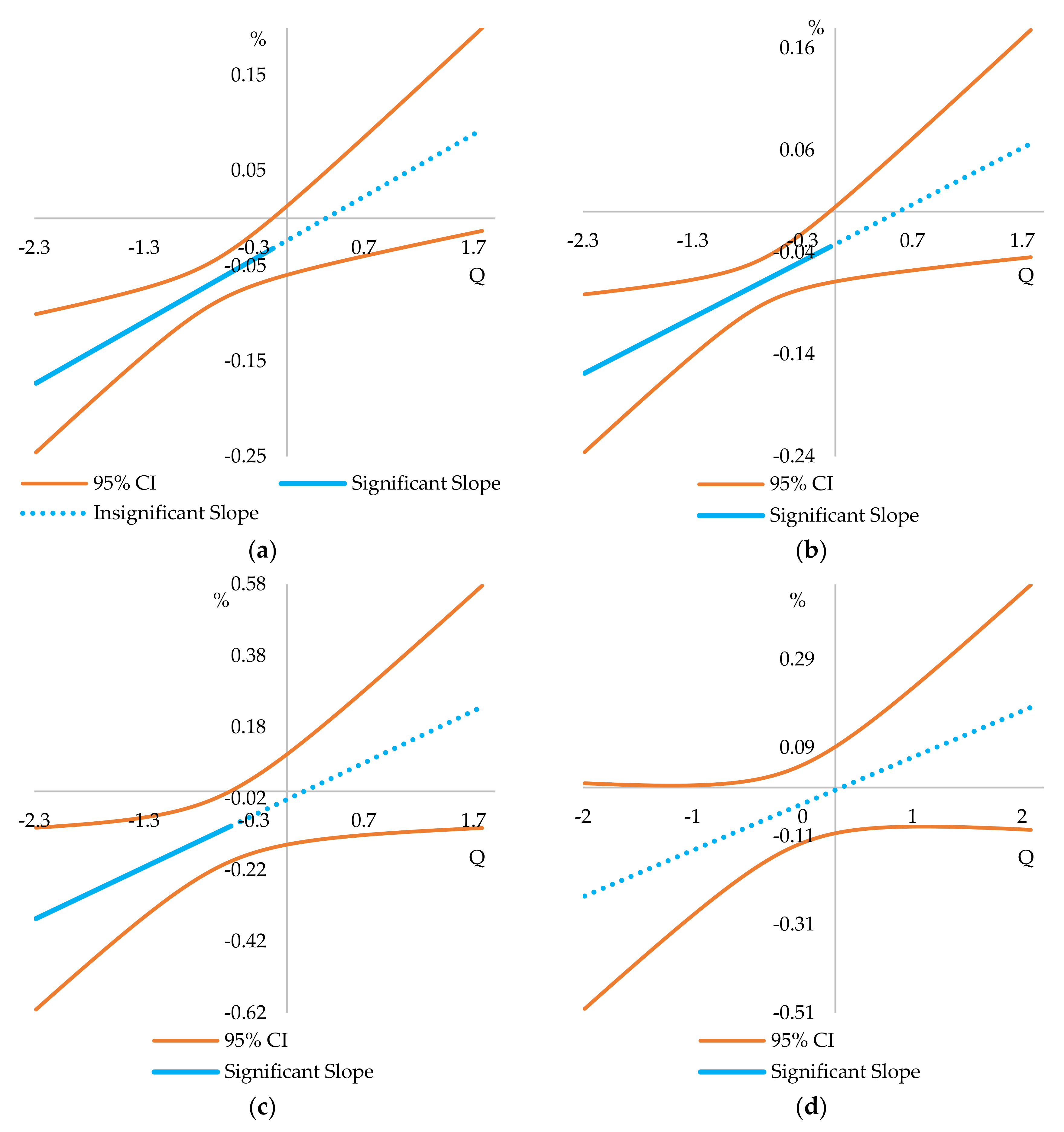
Figure 1 shows the conditional economic and productivity growth outcomes of the CP at the NUTS 2 and 3 disaggregation level over the 2000–2006 programming period that are mediated by institutional quality.

The estimates show that institutional quality positively affects the growth outcomes of the CP, i.e., the likelihood of transferring CP commitments to growth and productivity is higher in regions characterised as having good institutions. The estimates also suggest that a relatively bad institutional environment is related to adverse and statistically significant growth outcomes of the CP. In contrast, the relatively good institutional environment is linked to positive but insignificant growth outcomes.

Comparing the estimated ranges of the $Q_{i,t}$ values, which condition different growth outcomes of the CP (see

Table 3. Ranges of $Q_{i,t}$ values that condition the different signs and significance of the estimated slope coefficient of $g{r}_{i,t}$ on $S_{i,t}$.

Programming Period	Outcome Variable	Disaggregation Level	Range of ${\mathit{Q}}_{\mathit{i}\mathbf{,}\mathit{t}}$ Values That Condition Negative and Significant Outcomes of Cohesion Policy	Range of ${\mathit{Q}}_{\mathit{i}\mathbf{,}\mathit{t}}$ Values That Condition Negative and Insignificant Outcomes of Cohesion Policy	Range of ${\mathit{Q}}_{\mathit{i}\mathbf{,}\mathit{t}}$ Values That Condition Positive and Insignificant Outcomes of Cohesion Policy	Range of ${\mathit{Q}}_{\mathit{i}\mathbf{,}\mathit{t}}$ Values That Condition Positive and Significant Outcomes of Cohesion Policy
2000–2006	Economic growth	NUTS 2	<−0.52	−0.52–0.16	>0.16	-
		NUTS 3	<−0.14	−0.14–0.36	>0.36	-
	Productivity growth	NUTS 2	-	<-0.05	>−0.05	-
		NUTS 3	<−0.06	−0.06 – 0.56	>0.56	-
2007–2013	Economic growth	NUTS 2	-	<−2.75	−2.75–−1.70	>−1.70
		NUTS 3	-	<−2.60	−2.60–−1.76	>−1.76
	Productivity growth	NUTS 2	-	-	>−2.37	>−2.37
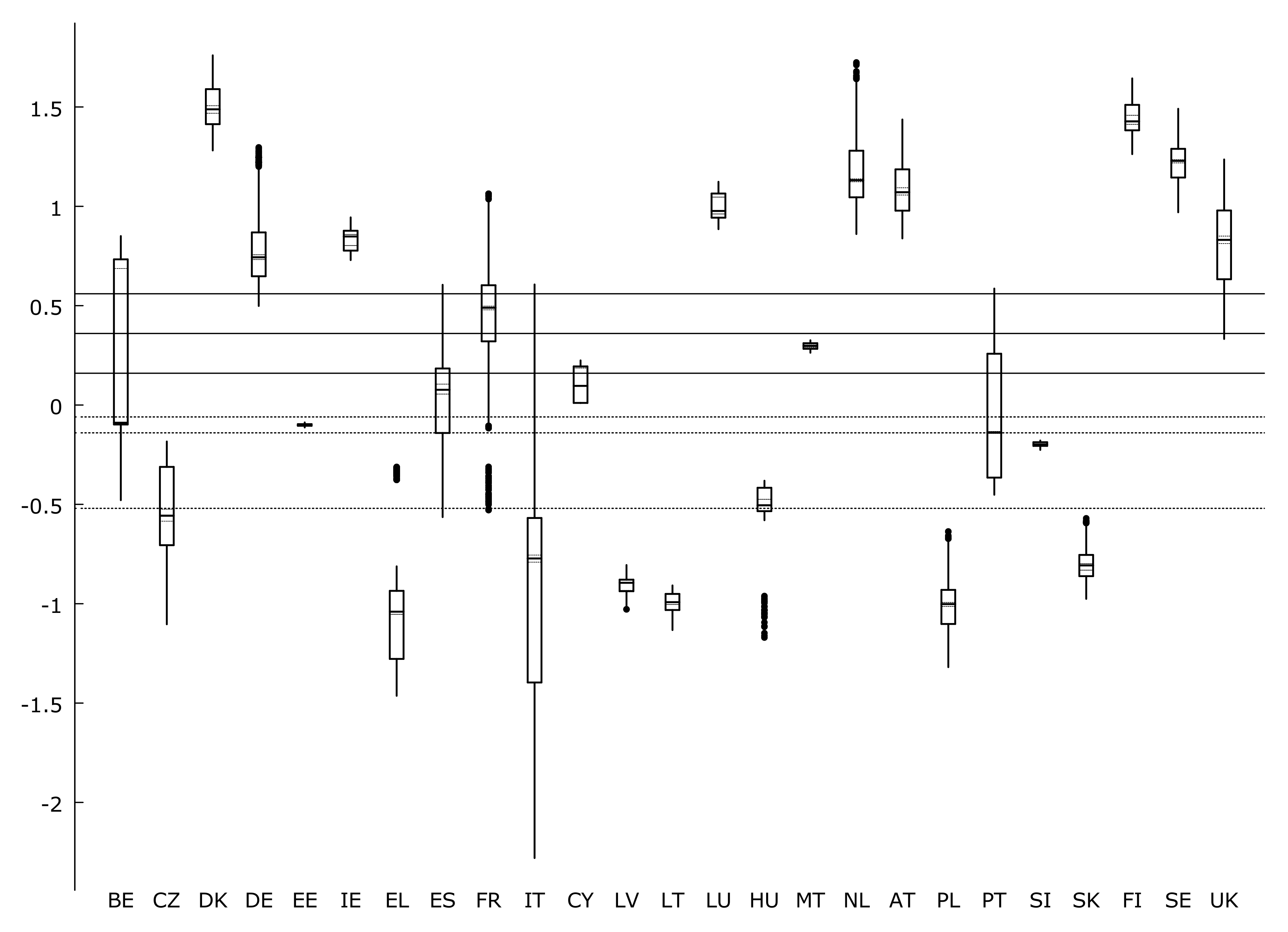
		NUTS 3	-	<−2.80	−2.80–−1.94	>−1.94

) with the distribution of the estimated $Q_{i,t}$ values over the 2000–2006 programming period (see Figure A1 in Appendix C.3.), we can conclude that (i) negative and significant growth outcomes of the CP were in all regions of Latvia, Lithuania, Poland, and Slovakia, in the majority regions of Italy and Greece—except for a few with untypically high (for a given country) $Q_{i,t}$ values—and in half of the regions of the Czech Republic and a few regions of Hungary with extremely low (for a given country) $Q_{i,t}$ values; (ii) positive but statistically insignificant growth outcomes of the CP were in all regions of Denmark, Ireland, the Netherlands, Austria, Finland, and Sweden, in the majority regions of Germany and the United Kingdom, as well as in a few regions of Belgium and France. Other countries/regions showed very mixed results depending on the outcome variable and disaggregation level under consideration.

Our findings are in line with [37] who revealed a positive but insignificant impact of the CP on productivity in EU–10 NUTS 1 regions and concluded that Southern EU countries (France, Greece, Italy, Portugal, and Spain) are less efficient in the management of the CP funds in comparison with Northern countries (Austria, Ireland, Finland, Germany, and the UK), although they received more cohesion investment. Our research results are also in line with [64] who revealed a positive but insignificant effect on growth in 70 NUTS 1 and 2 regions of Germany, Italy, and Spain, as well as with Becker et al. [17], since the authors concluded that almost all new EU MSs are not able to turn CP commitments into growth due to the insufficient level of institutional quality. Our results also support views of [5,6,41], who found that the significant adverse effect on growth and productivity depends on political behaviour and intervention, an area that could also be determined by political behaviour.

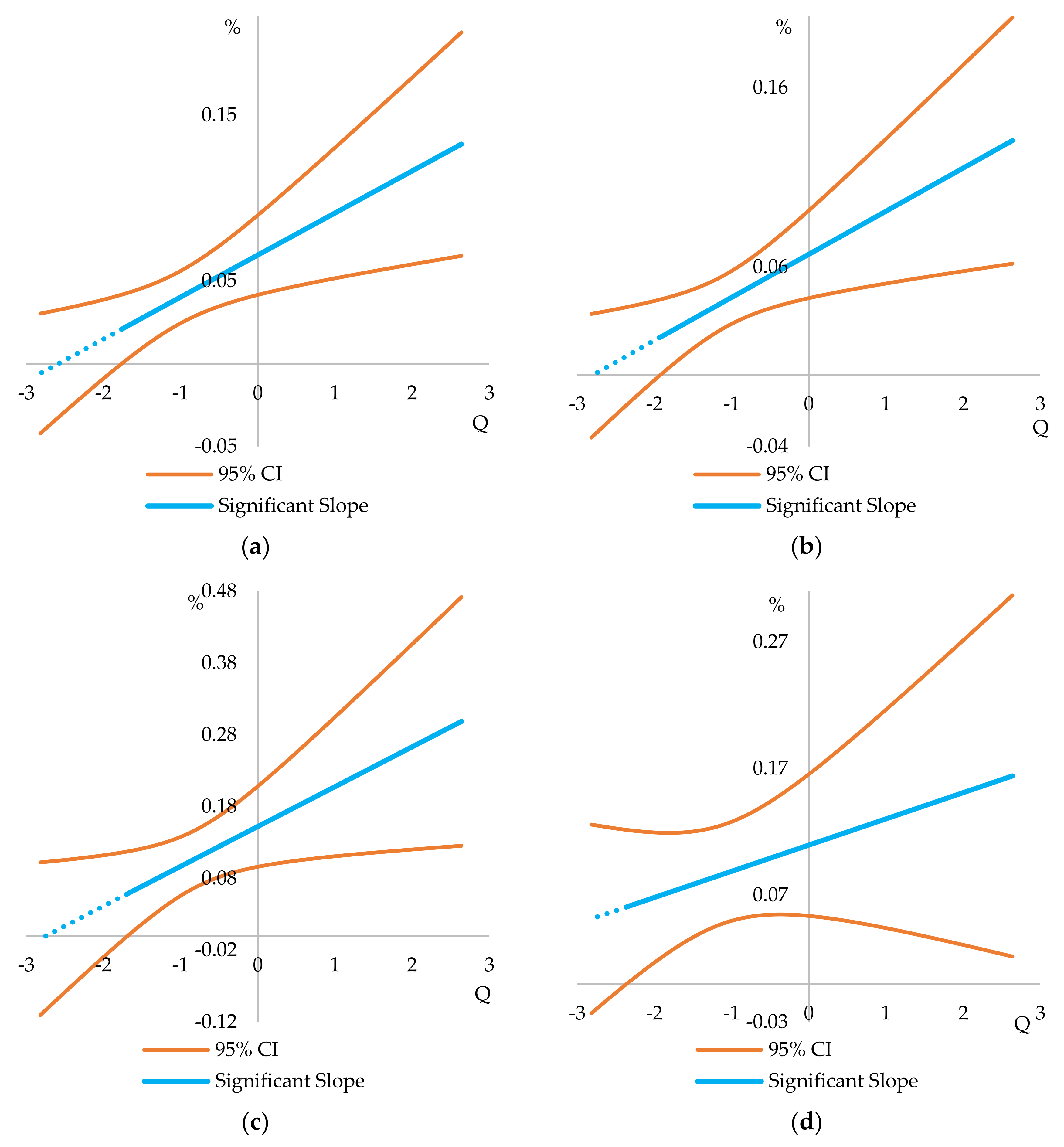
Figure 2 shows the conditional economic and productivity growth outcomes of the CP at the NUTS 2 and 3 disaggregation level over the 2007–2013 programming period that are mediated by institutional quality. As over the previous programming period, estimates show that institutional quality is positively related to the growth outcomes of the CP, i.e., better institutions in regions that receive CP support increase the likelihood to transfer investment into growth and productivity. The estimates suggest that relatively bad institutional environment is related to statistically insignificant outcomes of the CP, whereas the relatively good institutional environment is related to positive and statistically significant outcomes.

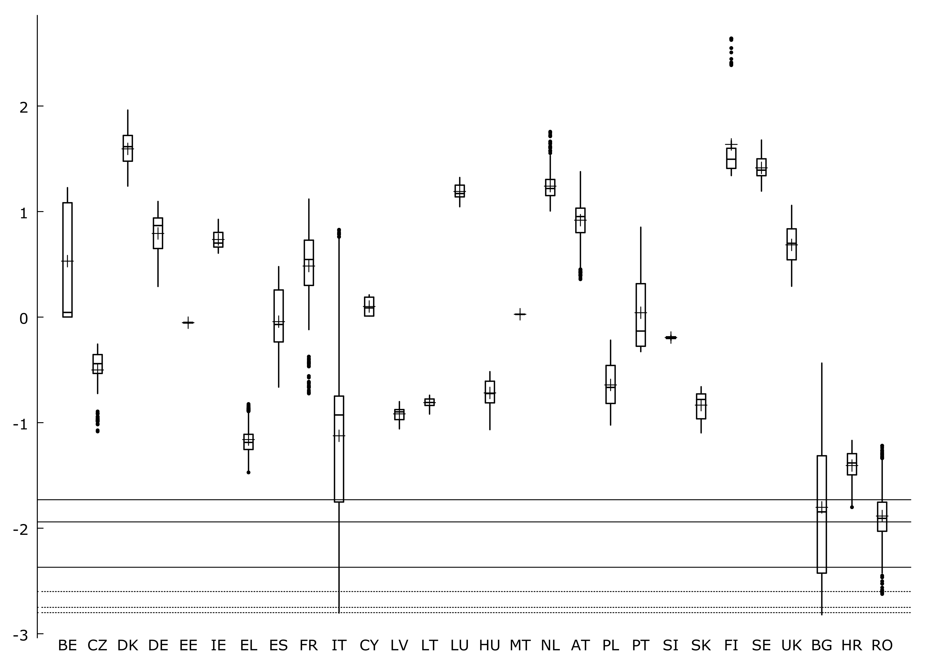
Comparing the estimated ranges of $Q_{i,t}$ values, which condition different growth outcomes of the CP (see Table 3) with the distribution of estimated $Q_{i,t}$ values over 2007–2013 programming period (see Figure A2 in Appendix C.3.), we can conclude that (i) insignificant growth outcomes of the CP were in almost all regions of Romania, except for a few with untypically high (for a given country) $Q_{i,t}$ values, in half the regions of Bulgaria and a few regions of Italy and Hungary with the extremely low (for a given country) $Q_{i,t}$ values; (ii) positive and significant growth outcomes of the CP were in all other countries/regions.

Our findings are in line with [39] who also found that although growth over 2007–2013 was negative, correlation between cohesion payments and growth was positive, and with those of [7] who revealed the positive significant growth outcomes over the 2007–2013 programming period in all NUTS 1 and 2 level regions in Portugal, Spain, Greece, Ireland, Belgium, France, Finland, Germany, Luxembourg, the Netherlands, Sweden, and the UK.

Comparing the 2000–2006 and 2007–2013 programming periods we, similarly to [3], can conclude that the CP for 2007–2013 had a more significant positive impact on economic and productivity growth. These facts allow us to argue that the estimated effect differs according to the programming period and suggests an improvement of the CP efficiency for 2007–2013 when compared to the previous programming period. Moreover, the positive influence of the CP is stronger in the regions with better institutional environment. This reveals a potential paradox of the CP that works better in the relatively more developed regions (which are also characterised as having a better institutional environment) compared to smaller (although still positive) gains for the most disadvantaged areas of the EU. This finding is also in line with [29,39].

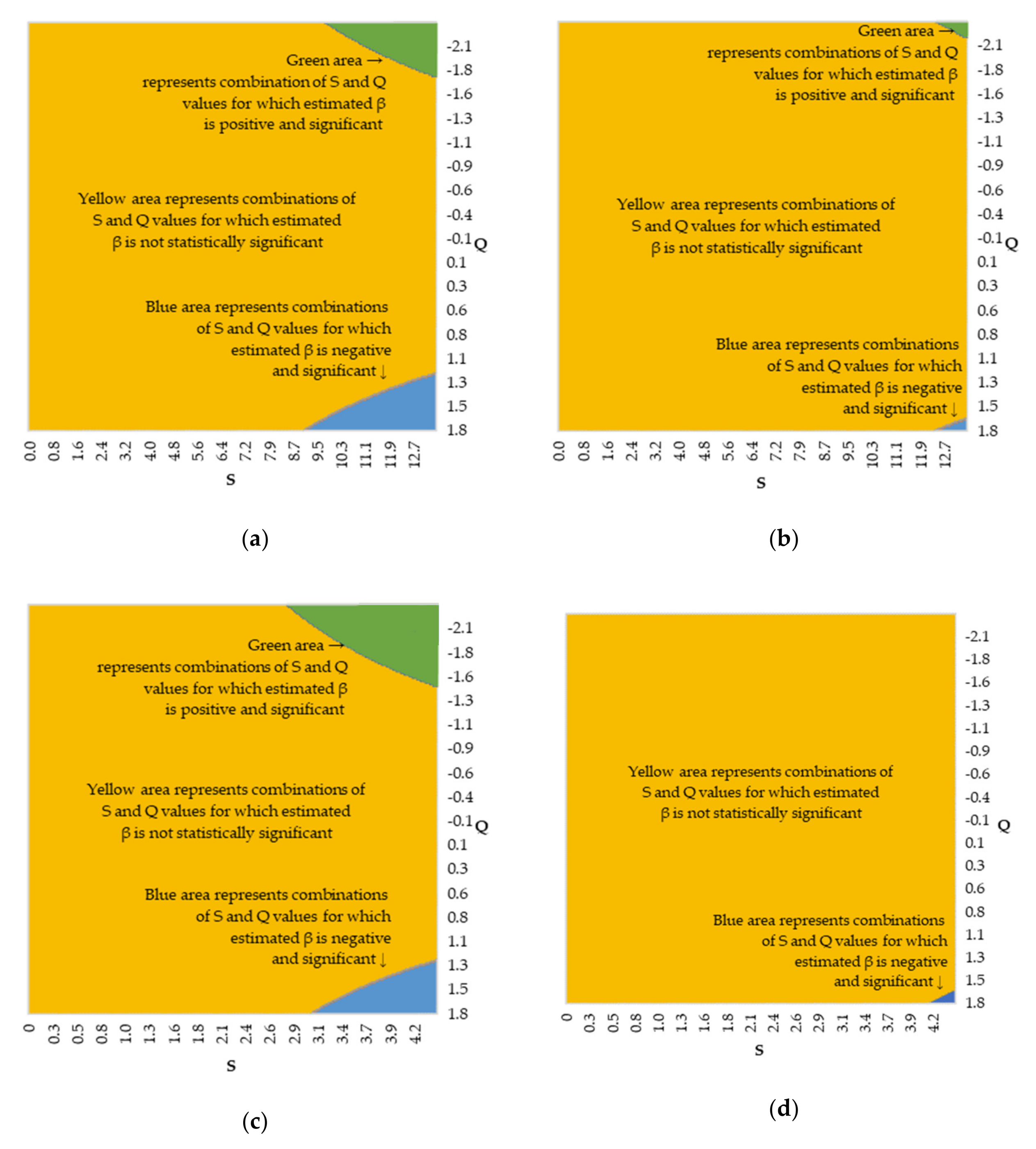
Figure 3 shows the significance and direction of the conditional beta-convergence that is mediated by the CP, institutional quality, and their interaction in terms of per capita GDP and productivity at the NUTS 2 and 3 disaggregation level over the 2000–2006 programming period.

The estimates show that the vast majority of combinations for $Q_{i,t}$ and $S_{i,t}$ over the observed range of values led to the insignificant convergence outcomes of the CP. We observe significant outcomes just if CP commitments are extremely intensive. Moreover, significant beta-convergence occurs in case of a relatively very favourable institutional environment and significant beta-divergence in case of a relatively very unfavourable institutional environment. The same is true for both dependent variables and both disaggregation levels under consideration. This suggests that a higher intensity of CP commitments positively mediates the significance of the CP convergence outcomes, whereas the institutional environment mediates whether there are positive or negative convergence outcomes. We find that the statistically significant negative convergence outcomes of the CP over the 2000–2006 programming period were in Greece, which is characterised by a high intensity of CP funding and low institutional quality. No region had a combination of high $Q_{i,t}$ and $S_{i,t}$ values over the 2000–2006 programming period that would fall into the range of a statistically significant positive impact on convergence.

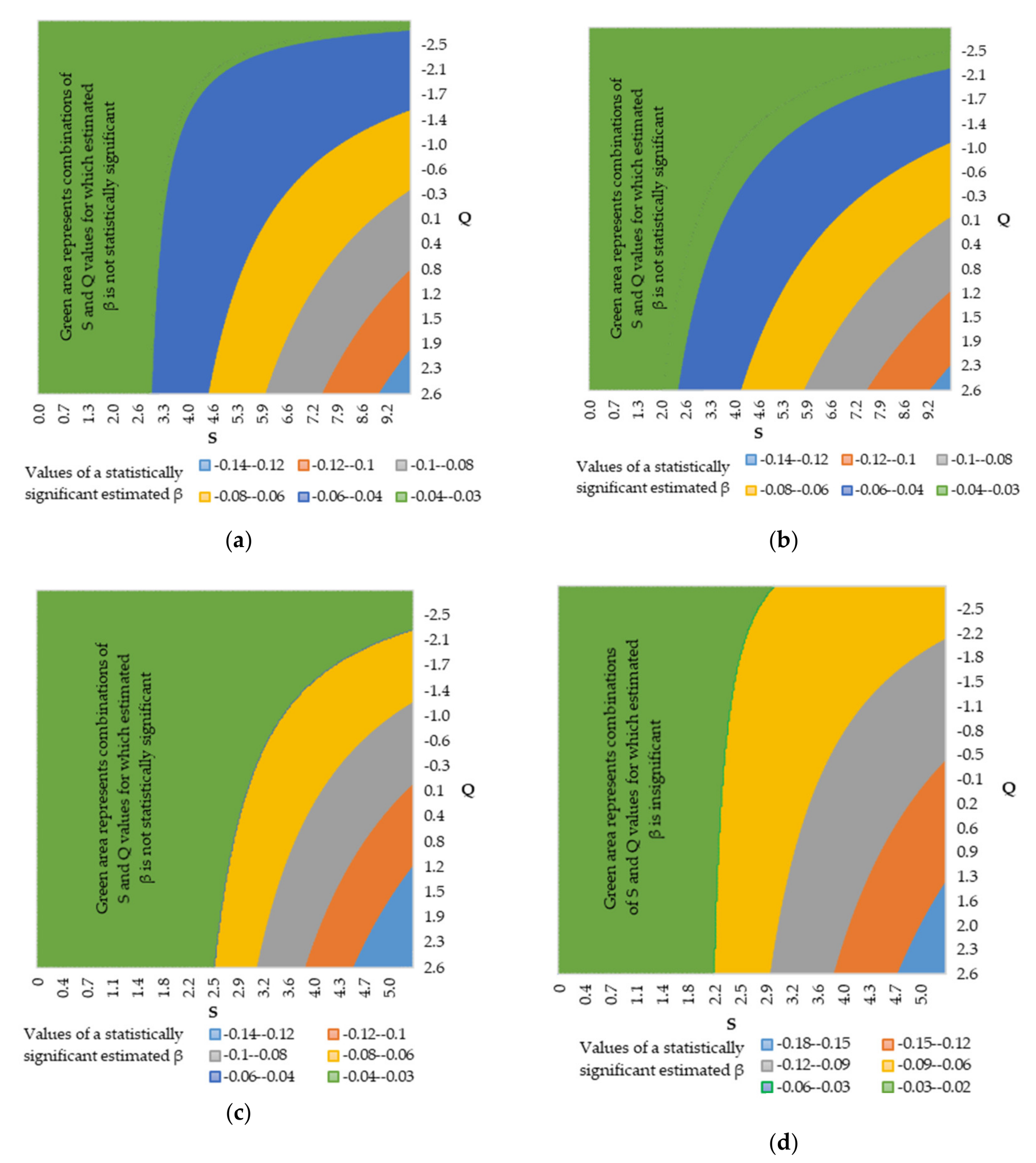
Figure 4 shows the significance direction and speed of the conditional beta-convergence in terms of per capita GDP and productivity at the NUTS 2 and 3 disaggregation level over the 2007–2013 programming period, which is mediated by the CP, institutional quality, and their interaction.

The estimates suggest that, compared with the previous programming period, the number of observed combinations of values for $Q_{i,t}$ and $S_{i,t}$, which led to the significant convergence outcomes of the CP, is much bigger. The estimates also show that the statistically significant estimated slope coefficients of $g{r}_{i,t\to T}$ on $Y_{i,t}$ are always negative, i.e., no observed combination of values for $Q_{i,t}$ and $S_{i,t}$ led to conditional beta-divergence. This suggests that CP induced convergence in terms of per capita GDP and productivity in a much bigger number of EU regions over 2007–2013 compared to the 2000–2006 programming period. Furthermore, the higher intensity of CP commitments and a more favourable institutional environment generate a bigger (in absolute terms) β coefficient, i.e., leads to faster convergence.

We find that CP had a minor positive impact on convergence for core regions in Austria, Belgium, Denmark Finland, France, Germany, Ireland, the Netherlands, Sweden and the UK, since their funding intensity was relatively low while the development level and the level of the institutional quality were among the highest in the EU. Less developed regions in the abovementioned countries, which were more intensively funded and had a high level on institutional quality, experienced one of the most fruitful convergence outcomes of the CP among the EU regions. The weak convergence of just a few regions of Hungary, Romania, Italy, Portugal, Greece and Spain was positively affected by the CP and it was due to the extremely high level of funding intensity despite the low level of institution quality. The rest of the regions in these countries experienced the statistically insignificant convergence outcomes of the CP, since a low level of funding intensity did not offset failures due to low-quality institutional environment. Regions of Croatia, the Czech Republic, Estonia, Latvia, Lithuania, Poland, Slovakia and Slovenia, despite their mid-level institutional environment, were experiencing the average convergence outcomes of the CP due to relatively intense funding.

The estimation results show that CP and institutional quality act, at some point, as the substituting mediating factors of conditional beta-convergence, i.e., the same β is estimated, i.e., the same speed of convergence can be reached in regions with a low intensity of CP commitments and favourable institutional environment, as well as in the regions with a high intensity of CP commitments and relatively unfavourable institutional environment. This reveals there is no potential paradox in the CP that generates the same convergence outcomes in the relatively less developed regions (that are also characterised as having a less favourable institutional environment) if they are more intensively financed as in the relatively more developed regions (that are also characterised as having more favourable institutional environment) if they are less intensively financed. It can be added that the substituting effect between the CP and institutional quality is diminishing, i.e., substitution between these two mediating factors has its limits.

Finding the evidence of a substituting effect does not mean that CP funding (money) can buy institutional quality (efficiency), i.e., that the two are interchangeable. We do not propose for policymakers to direct more CP transfers to poor-IQ regions as a form of “reward” for the less capable and/or, presumably, more corrupt regions. In light of our other findings, in which CP and IQ are shown as complementary for growth (their interaction term is positive and significant in both the programming periods), the policy advice is that CP transfers should be directed towards “good governance” regions. Moreover, if CP funds are directed to poor-IQ regions, these, in the first place, should be used to improve the overall institutional quality and only after that used for other purposes. The substitution effect that we find means that the same convergence effect could be reached by transferring more funds to regions with a relatively poor IQ as by transferring fewer funds to regions with a relatively good IQ, and suggests that a good IQ increases the efficiency of the funding. Even more, it suggests that CP transfers to poor-IQ regions create an effect of a dummy convergence by only increasing regional GDP as an additional expenditure in the region, which disappears when the funding ends, since it does not have a long-lasting effect on growth.

5. Conclusions

Our paper contributes to the methodological approaches used to estimate the outcomes of the CP by augmenting a traditional conditional beta-convergence model with a 3-way multiplicative term. We have shown that this specification could be used not only to examine the effect of the mediating factors on the growth outcomes of the CP but also on the convergence outcomes. Contrary to previously applied specifications with a 2-way multiplicative term, which only allowed to indirectly estimate the effect of the CP on convergence, our approach contributes to the direct estimation of the variability of the conditional beta-convergence coefficient, which depends on the intensity of the CP and a factor that could mediate the convergence outcomes of the CP. The suggested specification of the conditional beta-convergence model and the computation of conditional standard errors could contribute to the analysis of any mediating factor proxied by an interval/ratio variable.

Our empirical analysis aimed to estimate the mediating effect of institutional quality (which we assume is a crucial factor and connects other ones that mediate the outcomes of the CP) contributes to the evaluation of the growth and convergence outcomes of the CP, especially at the previously less analysed NUTS 3 level. Our empirical estimates based on conditional slopes and conditional standard errors contribute to explanting the sources of the heterogenous finding by previous research, which analyse different groups of regions and/or countries. We have shown that by computing the conditional marginal effects and their standard errors, we can find the positive and negative as well as significant and insignificant outcomes of the CP for different countries and/or regions.

The stability of the estimates (for all interaction terms) across spatial scales (levels of disaggregation) and across the dependent variables and programming periods is vital to robustly conclude that institutional quality plays a crucial role in determining the growth and convergence outcomes of the CP, which over the 2007–2013 programming period was much more successful in boosting growth and convergence compared to the previous one.

Our findings support the view that the direction, size, and significance of the effect of the CP commitment intensity on growth are conditional, i.e., a more significant positive effect is more plausible in regions with a more favourable institutional environment and vice versa, and that a significant effect is more likely to occur in regions where institutional quality is far from being average. These findings coincide with previous research that reveals a potential paradox in the CP that works better in the relatively more developed regions, which are not the main target of the CP compared to the most disadvantaged areas of the EU primarily targeted by the CP.

Considering the convergence outcomes, we have found that both the CP and institutional quality positively condition convergence in terms of per capita GDP and productivity. We have shown that the more intense CP commitments accelerate convergence, and if the institutional environment is favourable, this acceleration is even more significant. Furthermore, both act like substituting the mediating factors of the conditional beta-convergence with the diminishing marginal rate of substitution. This finding suggests that a higher intensity of cohesion payments could at some point compensate for an unfavourable institutional environment that hinders regional convergence and refutes the paradox of the CP.

Nevertheless, a higher intensity of CP commitments in the most disadvantaged (with the relatively unfavourable institutional environment) areas of the EU, aiming to speed-up the catch-up process, is not justified. Concerning the CP dilemmas: how much to spend and where, whether to “help the needy” or to “reward the able”, or whether to favour growth or convergence, our suggestions are as follows: (i) although boosting growth does not necessarily mean speeding-up the convergence, directing more CP funds towards regions with good IQ would help to achieve both goals. However, the primary focus should be on the convergence outcome; and (ii) CP funds should first be directed to improve IQ in the least developed regions and only later for other purposes.

The main limitations of our study that could be addressed in future research, using the developed specifications, are related to (i) assumptions made to quantify institutional quality at the NUTS 3 disaggregation level; (ii) the examination of the effect of other mediating factors on the outcomes of the CP; and (iii) testing the sensitivity of the findings to different estimation strategies. For example, since the 2007–2013 period covers the huge crisis in the Eurozone, which was highly asymmetric across countries and regions, many regions experienced negative growth rates. Perhaps an estimation split, running the model separately for cases of positive growth and cases of negative growth, would provide more information about whether the estimated effect of the CP is stronger because of “more policy effectiveness” or rather because of the nature of the growth-rate evolutions across space during the Eurozone crisis. The discussion about the country-cases and different country experiences also could be enriched by interacting the policy variables with a set of country fixed-effects.

References

1. Ciani, E.; de Blasio, G. European structural funds during the crisis: Evidence from Southern Italy. IZA J. Labour Policy 2015, 4, 1–31. [Google Scholar] [CrossRef] [Green Version]
2. Di Cataldo, M. The impact of EU Objective 1 funds on regional development: Evidence from the UK and the prospect of Brexit. J. Reg. Sci. 2017, 57, 814–839. [Google Scholar] [CrossRef]
3. Becker, S.O.; Egger, P.; von Ehrlich, M. Effects of EU Regional Policy: 1989-2013. Reg. Sci. Urban Econ. 2018, 69, 143–152. [Google Scholar] [CrossRef]
4. Coppola, G.; Destefanis, S. Structural Funds and Regional Convergence: Some Sectoral Estimates for Italy. In Geographical Labor Market Imbalances. AIEL Series in Labour Economics; Mussida, C., Pastore, F., Eds.; Springer: Berlin/Heidelberg, Germany, 2015. [Google Scholar]
5. Dotti, N.F. Unwritten Factors Affecting Structural Funds: The Influence of Regional Political Behaviours on the Implementation of EU Cohesion Policy. Eur. Plan. Stud. 2016, 24, 530–550. [Google Scholar] [CrossRef] [Green Version]
6. Pontarollo, N. Does Cohesion Policy affect regional growth? New evidence from a semi-parametric approach. In EU Cohesion Policy; Bachtler, J., Berkowitz, P., Hardy, S., Muravska, T., Eds.; Routledge: Abingdon, UK, 2017; pp. 93–108. [Google Scholar]
7. Pinho, C.; Varum, C.; Antunes, M. Structural Funds and European Regional Growth: Comparison of Effects among Different Programming Periods. Eur. Plan. Stud. 2015, 23, 1302–1326. [Google Scholar] [CrossRef] [Green Version]
8. Pinho, C.; Varum, C.; Antunes, M. Under What Conditions Do Structural Funds Play a Significant Role in European Regional Economic Growth? Some Evidence from Recent Panel Data. J. Econ. Issues 2015, 49, 749–771. [Google Scholar] [CrossRef] [Green Version]
9. Maynou, L.; Saez, M.; Kyriacou, A.; Bacaria, J. The Impact of Structural and Cohesion Funds on Eurozone Convergence, 1990–2010. Reg. Stud. 2016, 50, 1127–1139. [Google Scholar] [CrossRef]
10. Pellegrini, G.; Cerqua, A. Measuring the impact of intensity of treatment using RDD and covariates: The case of Structural Funds. In Proceedings of the 57th RSA Annual Conference, Bocconi University, Milan, Italy, 20–22 October 2016. [Google Scholar]
11. Gagliardi, L.; Percoco, M. The impact of European Cohesion Policy in urban and rural regions. Reg. Stud. 2017, 51, 857–868. [Google Scholar] [CrossRef]
12. Piętak, L. Did Structural Funds Affect Economic Growth and Convergence Across Regions? Spanish Case in the Years 1989–2016. INE PAN Work Pap. Ser. 2018, p. 44. Available online: http://inepan.pl/wp-content/uploads/2016/07/working-papers-44-Hiszpania-Pietak.pdf. (accessed on 20 November 2019).
13. Pellegrini, G.; Busillo, T.; Muccigrosso, T.; Tarola, O.; Terribile, F. Measuring the Impact of the European Regional Policy on Economic Growth: A Regression Discontinuity Design Approach. Pap. Reg. Sci. 2013, 92, 217–233. [Google Scholar] [CrossRef]
14. Di Cataldo, M.; Monastiriotis, V. An Assessment of EU Cohesion Policy in the UK Regions: Direct Effects and the Dividends of Targeting; LEQS–LSE ‘Europe in Question’ Discussion Paper Series 135; European Institute, LSE: London, UK, 2018; Available online: http://www.lse.ac.uk/European-institute/Assets/Dokuments/LEQS-Discussion-Papers/LEQSPaper135.pdf (accessed on 20 November 2019).
15. Kutan, A.M.; Yigit, T.M. European integration, productivity growth and real convergence. Eur. Econ. Rev. 2007, 51, 1370–1395. [Google Scholar] [CrossRef] [Green Version]
16. Kyriacou, A.P.; Roca-Sagales, O. The Impact of EU Structural Funds on Regional Disparities within Member States. Environ. Plan. C Politics Space 2012, 30, 267–281. [Google Scholar] [CrossRef] [Green Version]
17. Becker, S.O.; Egger, P.; von Ehrlich, M. Absorptive Capacity and the Growth and Investment Effects of Regional Transfers: Regression Discontinuity Design with Heterogeneous Treatment Effects. Am. Econ. J. Econ. Policy 2013, 5, 29–77. [Google Scholar] [CrossRef] [Green Version]
18. Rodríguez-Pose, A.; Garcilazo, E. Quality of Government and the Returns of Investment: Examining the Impact of Cohesion Expenditure in European Regions. Reg. Stud. 2015, 49, 1274–1290. [Google Scholar] [CrossRef]
19. Arbolino, R.; Boffardi, R. The Impact of Institutional Quality and Efficient Cohesion Investments on Economic Growth Evidence from Italian Regions. Sustainability 2017, 9, 1432. [Google Scholar] [CrossRef] [Green Version]
20. Jones, G.; Potrafke, N. Human capital and national institutional quality: Are TIMSS, PISA, and national average IQ robust predictors? Intelligence 2014, 46, 148–155. [Google Scholar] [CrossRef] [Green Version]
21. Fakher, A. Quality of institutions and integration in the world economy: Applied study on Egypt. J. Econ. Bus. 2014, 17, 69–96. [Google Scholar]
22. Ellis, J.A.; Smith, J.D.; White, R.M. Corruption and Corporate Innovation. Forthcom. J. Financ. Quant. Anal. 2015. Available online: http://dx.doi.org/10.2139/ssrn.2862128 (accessed on 20 August 2019).
23. Jude, C.; Levieuge, G. Growth Effect of Foreign Direct Investment in Developing Economies: The Role of Institutional Quality. World Econ. 2016, 40, 715–742. [Google Scholar] [CrossRef]
24. Boudreaux, C.J. Institutional quality and innovation: Some cross-country evidence. J. Entrep. Public Policy 2017, 6, 26–40. [Google Scholar] [CrossRef]
25. Alvarez, I.C.; Barbero, J.; Rodriguez-Pose, A.; Zofio, J.L. Does institutional quality matter for trade? Institutional conditions in a sectoral trade framework. World Dev. 2018, 103, 72–87. [Google Scholar] [CrossRef]
26. Rodríguez-Pose, A.; Novak, K. Learning processes and economic returns in European Cohesion Policy. Investig. Reg. 2013, 25, 7–26. [Google Scholar]
27. Brambor, T.; Clark, W.; Golder, M. Understanding Interaction Models: Improving Empirical Analyses. Political Anal. 2006, 14, 63–82. [Google Scholar] [CrossRef] [Green Version]
28. Falk, M.; Sinabell, F. The Effectiveness of Objective 1 Structural Funds in the EU 15: New Empirical Evidence from NUTS 3 Regions. In WIFO Working Papers 310; Austrian Institute of Economic Research (WIFO): Vienna, Austria, 2008; Available online: https://www.econstor.eu/bitstream/10419/128866/1/wp_310.pdf (accessed on 20 August 2019).
29. Fratesi, P.; Perucca, G. Territorial capital and the effectiveness of cohesion policies: An assessment for CEE Regions. Investig. Reg. J. Reg. Res. 2014, 29, 165–191. [Google Scholar]
30. Solow, R.M. A contribution to the theory of economic growth. Q. J. Econ. 1956, 70, 65–94. [Google Scholar] [CrossRef]
31. Swan, T.W. Economic Growth and Capital Accumulation. Econ. Rec. 1956, 32, 334–361. [Google Scholar] [CrossRef]
32. Romer, P.M. Endogenous technological change. J. Political Econ. 1990, 98, S71–S102. [Google Scholar] [CrossRef] [Green Version]
33. Romer, P.M. The Origins of Endogenous growth. J. Econ. Perspect. 1994, 8, 3–22. [Google Scholar] [CrossRef] [Green Version]
34. Nguyen, C.T.; Trinh, L.T. The impact of public investment on private investment and economic growth: Evidence from Vietnam. J. Asian Bus. Econ. Stud. 2018, 25, 15–32. [Google Scholar] [CrossRef] [Green Version]
35. Fujita, M.; Krugman, P.; Venables, A.J. The Spatial Economy: Cities, Regions and International Trade; MIT Press: Cambridge, MA, USA, 1999. [Google Scholar]
36. Bouayad-Agha, S.; Turpinn, N.; Védrine, L. Fostering the Development of European Regions: A Spatial Dynamic Panel Data Analysis of the Impact of Cohesion Policy. Reg. Stud. 2013, 47, 1573–1593. [Google Scholar] [CrossRef]
37. Gómez-García, J.; Enguix, M.D.R.M.; Gómez-Gallego, J.C. Estimations of the efficiency of structural funds: A parametric and nonparametric approach. Appl. Econ. 2012, 44, 3935–3954. [Google Scholar] [CrossRef]
38. Host, A.; Zaninović, V.; Krešimir, P. Cohesion Policy Instruments and Economic Growth: Do Institutions Matter? Ekon. Misao Praksa 2017, 2, 541–559. [Google Scholar]
39. Crescenzi, R.; Giua, M. The EU Cohesion Policy in Context: Regional Growth and the Influence of Agricultural and Rural Development Policies; LSE ‘Europe in Question’ Discussion Paper Series 2014, 85/2014, 1–50; University of Pittsburgh: Pittsburgh, PA, USA; Available online: http://aei.pitt.edu/93663/ (accessed on 20 November 2019).
40. Kyriacou, A.P. Ethnic segregation and the quality of government: The importance of regional diversity. Const. Political Econ. 2012, 23, 166–180. [Google Scholar] [CrossRef]
41. Eberle, J.; Brenner, T. More bucks, more growth, more justice? The effects of regional structural funds on regional economic growth and convergence in Germany. Work. Pap. Innov. Space. 16 January 2016. Available online: https://www.econstor.eu/handle/10419/147971 (accessed on 20 November 2019).
42. Dias, J.; Tebaldi, E. Institutions, Human Capital, and Growth: The Long-run Institutional Mechanism. Struct. Chang. Econ. Dyn. 2012, 23, 300–312. [Google Scholar] [CrossRef]
43. Bouzahzah, M.; Simplice, S.A.; Jellal, M. Institutional Governance, Education and Growth. Theor. Econ. Lett. 2016, 6, 131–137. [Google Scholar] [CrossRef] [Green Version]
44. Wang, Y.; Cheng, L.; Wang, H.; Li, L. Institutional quality, financial development and OFDI. Pac. Sci. Rev. 2014, 16, 127–132. [Google Scholar] [CrossRef] [Green Version]
45. Ma, J.; Lu, Y. Free Trade or Protection: A Literature Review on Trade Barriers. Res. World Econ. 2011, 2, 69–70. [Google Scholar] [CrossRef]
46. Anderson, J.E.; Marcouiller, D. Insecurity and the pattern of trade: An empirical investigation. Rev. Econ. Stat. 2002, 84, 342–352. [Google Scholar] [CrossRef] [Green Version]
47. Estrada, G.; Park, D.; Ramayandi, A. Financial Development, Financial openness, and Economic growth. Adb Econ. Work. Pap. Ser. 2015, p. 442. Available online: https://papers.ssrn.com/sol3/papers.cfm?abstract_id=2707518 (accessed on 20 August 2019).
48. Benáček, V.; Lenihan, H.; Andresso-O’Callaghan, B.; Michalíková, E. Political Risk, Institutions and Foreign Direct Investment: How Do They Relate in Various European Countries? World Econ. 2013, 37, 625–653. [Google Scholar] [CrossRef] [Green Version]
49. Aziz, O.G. Institutional quality and FDI inflows in Arab economies. Financ. Res. Lett. 2018, 25, 111–123. [Google Scholar] [CrossRef]
50. Arpaia, A.; Mourre, G. Institutions and Performance in European Labour Markets: Taking a gresh look at evidence. Econ. Pap. 2009, 391. [Google Scholar] [CrossRef] [Green Version]
51. Grigoli, F.; Mills, Z. Institutions and Public investment: An empirical analysis. Econ. Gov. 2014, 15, 131–153. [Google Scholar] [CrossRef]
52. Alesina, A.; Zhuravskaya, E. Segregation and the quality of government in a cross-section of countries. Am. Econ. Rev. 2011, 101, 1872–1911. [Google Scholar] [CrossRef] [Green Version]
53. Henderson, J.V.; Wang, H.G. Urbanization and city growth: The role of Institutions. Reg. Sci. Urban Econ. 2007, 37, 283–313. [Google Scholar] [CrossRef]
54. Dellmuth, L.M.; Schraff, D.; Stoffel, M.F. Distributive Politics, Electoral Institutions and European Structural and Investment Funding: Evidence from Italy and France. J. Common Mark. Stud. 2017, 55, 275–293. [Google Scholar] [CrossRef] [Green Version]
55. Olson, M. The Logic of Collective Action: Public Goods and the Theory of Groups; Harvard University Press: Cambridge, MA, USA; London, UK, 1965. [Google Scholar]
56. Beugelsdijk, M.S.; Eijffinger, S.C.W. The effectiveness of structural policy in the European Union: An empirical analysis for the EU-15 in 1995–2001. J. Common Mark. Stud. 2005, 43, 37–51. [Google Scholar] [CrossRef] [Green Version]
57. Mo, P.H. Corruption and Economic Growth. J. Comp. Econ. 2001, 29, 66–70. [Google Scholar] [CrossRef] [Green Version]
58. Cerqua, A.; Pellegrini, G. Are we spending too much to grow? The case of Structural Funds. J. Reg. Sci. 2018, 58, 535–563. [Google Scholar] [CrossRef]
59. Wright, G. Linear Models for Evaluating Conditional Relationship. Am. J. Political Sci. 1976, 20, 349–373. [Google Scholar] [CrossRef]
60. Friedrich, R. In Defense of Multiplicative Terms in Multiple Regression Equations. Am. J. Political Sci. 1982, 26, 797–833. [Google Scholar] [CrossRef]
61. Leona, A.; West, S. Multiple Regression: Testing and Interpreting Interactions; Sage: London, UK, 1991. [Google Scholar]
62. Rodríguez-Pose, A.; Fratesi, U. Between Development and Social Policies: The Impact of European Structural Funds in Objective 1 Regions. Reg. Stud. 2004, 38, 97–113. [Google Scholar] [CrossRef]
63. Butkus, M.; Cibulskiene, D.; Maciulyte-Sniukiene, A.; Matuzeviciute, K. What Is the Evolution of Convergence in the EU? Decomposing EU Disparities up to NUTS 3 Level. Sustainability 2018, 10, 1552. [Google Scholar] [CrossRef] [Green Version]
64. Florio, M.; Moretti, L. The Effect of Business Support on Employment in Manufacturing: Evidence from the European Union Structural Funds in Germany, Italy and Spain. Eur. Plan. Stud. 2014, 22, 1802–1823. [Google Scholar] [CrossRef]
65. Mohl, P.; Hagen, T. Does EU cohesion policy promote growth? Evidence from regional data and alternative econometric approaches. Zew Discuss. Pap. 2008, 8–86. [Google Scholar] [CrossRef] [Green Version]
66. Wostner, P.; Šlander, S. The effectiveness of EU cohesion policy revisited: Are EU funds really additional? Eur. Policies Res. Cent. 2009, 69, 1–26. [Google Scholar]
67. Becker, S.O.; Egger, P.; von Ehrlich, M.; Fenge, R. Going NUTS–The effect of EU structural funds on regional performance. J. Public Econ. 2010, 94, 578–590. [Google Scholar] [CrossRef] [Green Version]
68. Mohl, P.; Hagen, T. Does EU structural funds promote regional growth? New evidence from various panel data approaches. Reg. Sci. Urban Econ. 2010, 40, 353–365. [Google Scholar] [CrossRef]
69. Varga, J.; Veld, J. A Model–Based Analysis of the Impact of Cohesion Policy Expenditure 2000–06: Simulations with QUEST III endogenous R&D model. Econ. Model. 2010, 28, 647–663. [Google Scholar] [CrossRef] [Green Version]
70. Accetturo, A.; de Blasio, G.; Ricci, L. A tale of unwanted outcome: Transfers and local endowments of trust and cooperation. J. Econ. Behav. Organ. 2014, 102, 74–89. [Google Scholar] [CrossRef]
71. European Commission. Measuring the impact of Structural and Cohesion Funds using regression discontinuity design in EU27 in the period 1994-2011, Ex post evaluation of Cohesion Policy programmes 2007–2013, focusing on the European Regional Development Fund (ERDF) and the Cohesion Fund (CF). Final technical Report, Work Package 14c—Tasks 2 and 3. 2016. Available online: https://ec.europa.eu/regional_policy/sources/docgener/evaluation/pdf/expost2013/wp14c_task1_final_report_en.pdf (accessed on 15 July 2019).
72. Bondonio, D.; Pellegrini, G. Macro-economic effects of cohesion policy funding in 2007–2013 Executive Summary. Work Package 14c: Regression discontinuity design. Work Package 14d: Propensity score matching. Ex post evaluation of Cohesion Policy programmes 2007–2013, focusing on the European Regional Development Fund (ERDF) and the Cohesion Fund (CF). European Commission. Luxembourg: Publications Office of the European Union. 2016. Available online: https://ec.europa.eu/regional_policy/sources/docgener/evaluation/pdf/expost2013/wp14c_d_executive_summary_en.pdf (accessed on 15 July 2019).
73. SWECO. Final Report—ERDF and CF Regional Expenditure Contract. 2008. 2007.CE.16.0.AT.036. Available online: https://ec.europa.eu/regional_policy/sources/docgener/evaluation/pdf/expost2006/expenditure_final.pdf (accessed on 15 July 2019).
74. Ciffolilli, A.; Condello, S.; Pompili, M.; Roemish, R.; Geography of Expenditure. Final Report. Work Package 13. Ex post evaluation of Cohesion Policy programmes 2007–2013, focusing on the European Regional Development Fund (ERDF) and the Cohesion Fund (CF). 2015. Available online: https://ec.europa.eu/regional_policy/sources/docgener/evaluation/pdf/expost2013/wp13_final_report_en.pdf (accessed on 15 July 2019).
75. Charron, N.; Lapuente, V.; Rothstein, B. (Eds.) Measuring the Quality of Government and Subnational Variation. Report for the European Commission Directorate-General Regional Policy, Directorate Regional Policy; Quality of Quality of Government and Returns of Investment: Cohesion Expenditure in European Regions 1289 Government Institute, Department of Political Science, University of Gothenburg: Gothenburg, Sweden, 2010; Available online: http://ec.europa.eu/regional_policy/sources/docgener/studies/pdf/2010_government_1.pdf (accessed on 15 July 2019).
76. Charron, N.; Dijkstra, L.; Lapuente, V. Regional governance matters: Quality of government within European union member states. Reg. Stud. 2014, 48, 68–90. [Google Scholar] [CrossRef]
Figure 1. A range of estimated slope coefficients (slope) of g r i , t on S i , t according to the value of Q i , t and 95% confidence interval over the 2000–2006 programming period. A point on a slope shows an effect of 1% intensity of European Regional Development Fund (ERDF) and Cohesion Fund (CF) commitments on a growth rate for a particular value of Q i , t . (a) Represents conditional economic growth outcomes of the CP at the NUTS 3 disaggregation level. (b) Represents conditional productivity growth outcomes of the CP at the NUTS 3 disaggregation level. (c) Represents conditional economic growth outcomes of the CP at the NUTS 2 disaggregation level. (d) Represents conditional productivity growth outcomes of the CP at the NUTS 2 disaggregation level.
Sustainability 12 03025 g001
Figure 2. A range of estimated slope coefficients (slope) of g r i , t on S i , t according to the value of Q i , t and 95% confidence interval over the 2007–2013 programming period. A point on a slope shows an effect of 1% intensity of ERDF and CF commitments on a growth rate for a particular value of Q i , t . (a) Represents conditional economic growth outcomes of the CP at the NUTS 3 disaggregation level. (b) Represents conditional productivity growth outcomes of the CP at the NUTS 3 disaggregation level. (c) Represents conditional economic growth outcomes of the CP at the NUTS 2 disaggregation level. (d) Represents conditional productivity growth outcomes of the CP at the NUTS 2 disaggregation level.
Sustainability 12 03025 g002
Figure 3. Significance and sign of the estimated slope coefficients of g r i , t on Y i , t 1 according to the specific combination of values for Q i , t and S i , t over the 2000–2006 programming period, i.e., significance and sign of the conditional beta-convergence (or simply ‘β*100’ in a figure) mediated by CP and institutional quality. (a) Represents convergence outcomes of the CP in terms of per capita GDP at the NUTS 3 disaggregation level. (b) Represents convergence outcomes of the CP in terms of productivity at the NUTS 3 disaggregation level. (c) Represents convergence outcomes of the CP in terms of per capita GDP at the NUTS 2 disaggregation level. (d) Represents convergence outcomes of the CP in terms of productivity at the NUTS 2 disaggregation level.
Sustainability 12 03025 g003
Figure 4. Significance, sign, and size of the estimated slope coefficients of g r i , t on Y i , t 1 according to the specific combination of values for Q i , t and S i , t over the 2007–2013 programming period, i.e., significance, sign, and speed of the conditional beta-convergence (or simply ‘β*100’ in the figure) mediated by CP and institutional quality. (a) Represents convergence outcomes of the CP in terms of per capita GDP at the NUTS 3 disaggregation level. (b) Represents convergence outcomes of the CP in terms of productivity at the NUTS 3 disaggregation level. (c) Represents convergence outcomes of the CP in terms of per capita GDP at the NUTS 2 disaggregation level. (d) Represents convergence outcomes of the CP in terms of productivity at the NUTS 2 disaggregation level.
Sustainability 12 03025 g004