Analysis and Prediction of Land Use in Beijing-Tianjin-Hebei Region: A Study Based on the Improved Convolutional Neural Network Model

Abstract

During the rapid economic development of China, there are certain blind decisions made in the use of land resources, which poses a significant threat to sustainable development. With the help of the improved convolutional neural network model, this paper analyzes the land use of the Beijing-Tianjin-Hebei region of China from 1995 to 2018, and provides a prediction for 2023. The research results show that: (1) There is still much room for improvement in the land use of the Beijing-Tianjin-Hebei region, with dry land taking up the largest proportion of land in these three locations; (2) Beijing’s development has been well protected in terms of land use. It is predicted that by 2023, the proportions of its woodland, grassland, and rivers, lakes, reservoirs and ponds would increase by 0.26%, 0.30%, and 0.61%, respectively, compared with their proportion in 2018; (3) the land use type in Tianjin during the research period was generally stable. In 2018, the proportion of its woodland and grassland had increased by 1.04% and 0.61%, respectively, compared with that of 1995; and (4) many ecological and environmental problems were exposed during the construction of highways in Hebei province. The area of sand land, saline-alkali land, marshland, bare land, and bare rock areas have all increased, and their total proportion is predicted to reach 1.48% by 2023.

1. Introduction

Sustainable development can be defined as “development that can meet the needs of contemporary people without compromising the ability of future generations to meet their needs [1].” The sustainable development of a country or region also considers its land resource, which is a critical material basis for economic growth and social activities, and is of great significance to the sustainable development of the society, economy, and ecological environment. For example, Yang and Li studied the relationship between energy efficiency, ownership structure, and sustainable development in China [2]; Jónsson et al. used soil indicators for sustainable development [3]; Edrisi and Tripathi studied how to manage soil resources to realize sustainable development [4]; Asimeh et al. analyzed the consolidation plans for agricultural land use sustainability in southwest Iran [5]; and Yang and Li analyzed the efficiency of industrial waste gas control in China [6].

Since the 1990s, China has achieved world-renowned rapid development. However, in this process, driven by the motivation to seek short-term economic benefits, certain regions of China have made blind decisions in the use of land resources that is not scientific. For example, Khantachavana et al. studied the transaction values of land use rights in rural China [7]; Zoomers et al. analyzed acquiring and developing land safely [8]; Shen et al. studied how the healthcare system uses land [9]; and Mertz and Mertens studied the conservation and land sharing policies in developing countries [10]. Land is often over-developed amid rapid economic growth—resources are wasted, and the entire ecological environment suffers damages, as discussed below:

(1) The impact on soil and vegetation. The various emissions of industrial wastewater, waste gas and waste residue in the process of development have directly or indirectly polluted the soil, hurt the soil quality, caused damage to the existing land vegetation and microbial communities, and led to the degradation of land structure and land fertility, as well as soil salinification, soil acidification and soil hardening. For example, Reidsma et al. assessed the agricultural land use policies for Taihu Basin in China [11]; Lee et al. used a land use regression model to analyze the air pollution in Hong Kong [12]; Chen et al. studied the spatial and temporal changes in soil properties in the subtropical plain [13]; Li et al. researched the water environment management for the soil in central China [14]; and Yang and Li analyzed the efficiency of industrial wastewater control for soil protection [15]. Additionally, the blind and unscientific development of land resources in many areas has led to a decline in the vegetation coverage rate and the regeneration capacity of the plant community is greatly reduced; the plant diversity has been severely impacted, which will ultimately impair the self-adjustment capacity of the entire ecosystem. For example, Chandregowda et al. [16], Velasquez and Lavelle [17], and Yang and Li [18] used the increase of woody shrubs, soil macrofauna, and efficiency of water and energy to, respectively, conduct their studies.

(2) The impact on the ecological environment. During the rapid expansion of urban areas in China in recent years, a large amount of farmland and green land have been converted into building land. The infiltration of sewage has caused serious adverse effects on water resources and the water environment. For example, Li and Yang studied the total factor efficiency of China’s industrial coal input and wastewater control [19]; Lass et al. studied the contamination of wastewater for drinking water resources in China [20]; and Yuan and Yang studied how to optimize the electric power system to minimize sewage based on hybrid intelligent algorithms [21]. With the development of economy, the number of factories has soared, the urban population has become increasingly dense, and huge amounts of wastewater and waste gas are generated, posing a serious threat to the water environment and the atmospheric environment. The water pollution, caused by wastewater emissions, and air pollution, caused by waste gas emissions, have become the most severe challenge to China in recent years. For example, Wang et al. evaluated the land-cover change for urban planning and sustainability in Dongying city, China [22]; Li et al. studied the effects of regulation on air pollution in China [23]; and Yang et al. also researched air pollution control policies in the Yangtze River Delta cities, in China [24].

(3) The impact on people’s quality of life. In the process of economic development and urbanization, some areas of China have neglected the importance of a balanced and harmonious ecological environment in their pursuit of rapid economic development, which has eventually resulted in serious destruction of the ecological environment and decreasing urban green space. For example, Shi et al. focused on preventing future smog crises in China and globally [25]; Tong et al. studied the spatial flows of e-waste in China [26]; and Helbich et al. studied the street view green and blue spaces and their associations in Beijing, China [27]. The improper use of land resources has directly affected biological communities, underground water levels, and air quality. Once the ecological system is out of balance, it will greatly affect people’s quality of life. For example, Wei et al. discussed the progress of integrated assessment models for land use, climate policy, and ecological balance [28]; Gao et al. researched the environmental governance policies in China’s Pearl River Delta and their relationship with land use [29]; Hansen et al. discussed the progress of ecological civilization in China [30]; and Yang and Yang studied ecological governance policies in China from the perspective of evolutionary games [31].

The academic community has also studied the scientific development and utilization of land resources in China. For example, Ash and Edmonds analyzed the impact of China’s land-intensive methods on the increase of the agricultural output. They argue that China’s yields per hectare have remarkably increased through making full use of the natural environment, such as land resources, which has been a significant factor in Chinese agriculture progress since 1978 [32]. In the context of tightening of land development policies in China, Yang et al. took the Jiangbei National New Area in Nanjing as an example to study the development of China’s “National New Area” in recent years. The results of their research indicate that the commercialization of rural land is an important driver of China’s “National New Area” policy innovation, but this policy has not effectively solved the land-centric development crisis.

Moreover, the rapid development of the rural land market may put more burden on financialization in the near future [33]. Clarke studied the use of land resources in China from the perspective of ownership, and argued that the 70-year “long-term use right” of Chinese land and an ownership system based on full private payment are not significantly different. This research shows that the ownership of land resources reflects, and affects, China’s wealth distribution to a considerable extent. The government can influence this process by formulating new policies, but it must carefully measure the actual role it ultimately plays [34]. Ge et al. analyzed the changes in land use in China ’s poor areas between 2013 and 2018. Using Google Earth Engine to build a land-use change framework, and using Bayesian hierarchy model to analyze the spatial-temporal change pattern of land use, they showed that the arable land continues to decrease in poor areas in China, while the built-up land and vegetation are gradually expanding. Simultaneously, there is a clear difference between the deep poverty-stricken counties and the normal poverty-stricken counties in terms of cultivated land and built-up land [35]. Batunacun et al. studied land degradation in pastoral areas of China. Using the partial order theory and the Hasse diagram technique, they analyzed the factors leading to land degradation in pastoral areas using the Xilingol League in China as an example. The research results show that after 2000, urbanization gradually became the main cause of land degradation in pastoral areas. In addition, human disturbance and water condition were also important causes of land degradation in pastoral areas. Therefore, the Chinese government needs to adopt new policies to mitigate the impact of urbanization, in order to protect land resources in pastoral areas [36].

However, the existing literature still lacks a comprehensive long-term analysis of the changing trends of various types of land resources in China, and a scientific prediction of the future land use. Therefore, this paper has conducted a systematic analysis on the change in various types of green land, including woodland, shrubbery, sparse woodland, other woodland, high coverage grassland and medium coverage grassland, etc., as well as the change in various types of building land, including urban and town land, rural settlements, and other building land. This studies uses a convolutional neural network model, based on the land use data from 1995 to 2018, in the Beijing-Tianjin-Hebei region of China [37]. Additionally, after summarizing the historical land use data, this paper has predicted the land use in 2023. The reasons for choosing the Beijing-Tianjin-Hebei region as the research object include the following:

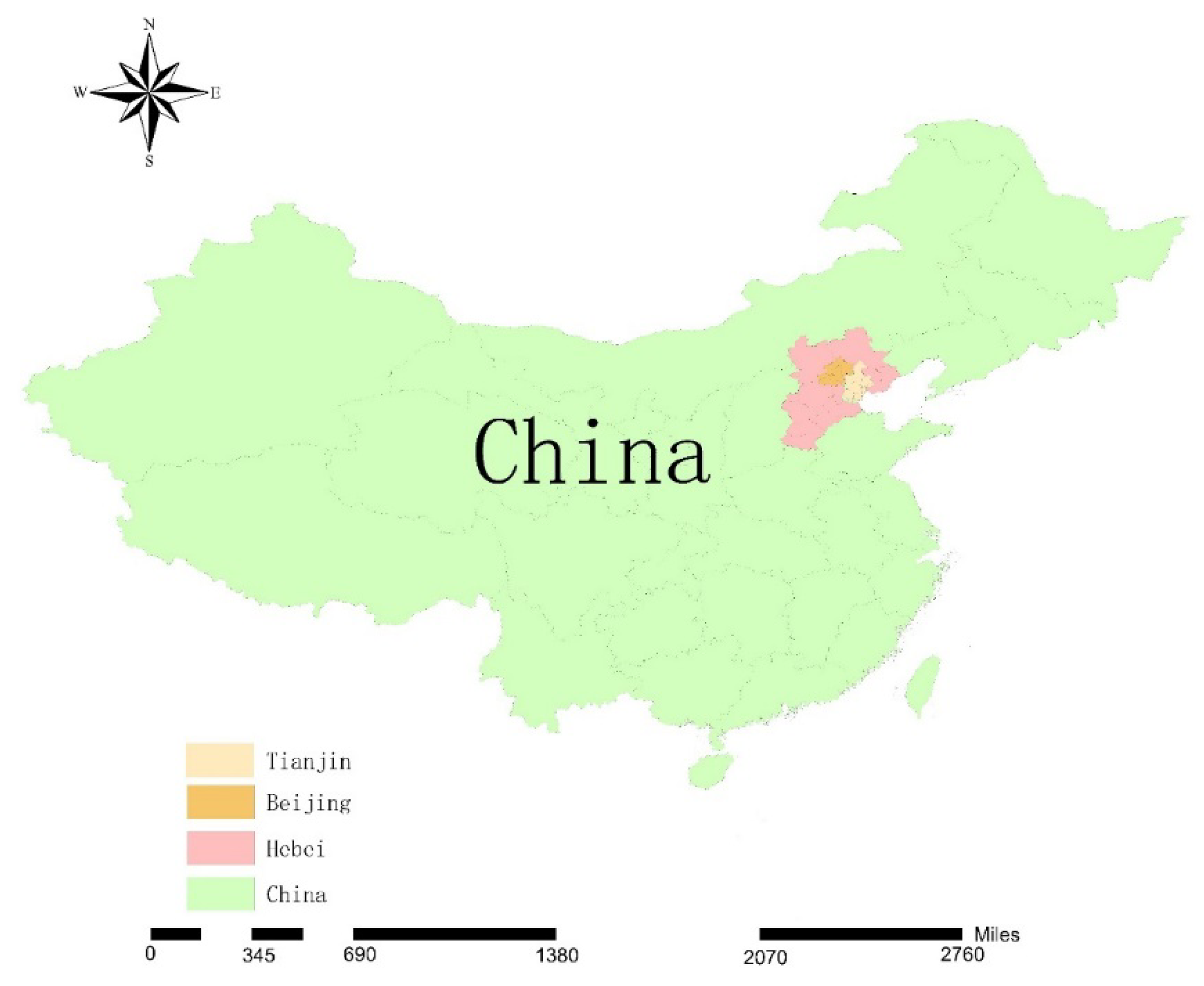
(1) The Beijing-Tianjin-Hebei region is of great significance to China’s development. The region is one of the core producers for Chinese economy: Not only does it contain the capital city of Beijing (the political and cultural center of China), but also includes Tianjin, one of the four municipalities directly under the central government in China. Moreover, this region also covers 11 cities of Hebei Province, with an area of approximately 218,000 square kilometers [38]. Thus, this region was considered an insightful subject for this study of China’s sustainable development (see Figure 1).

(2) The Beijing-Tianjin-Hebei region covers various typical land forms and vegetation types. The terrain of this region slopes from the northwest to the southeast. Mountains, hills and plateaus dominate the northwest region, while the middle and southeast regions are dominated by the vast Beijing-Tianjin-Hebei Plain, and the east region is adjacent to the Bohai Sea. The vegetation spread across the plains, flood alluvial plains, alluvial low plains, sloping flatlands, dunes, depressions, and coastal plains in this area all have fairly typical geographical characteristics [37]. Therefore, this region is ideal for the study of land resource use and vegetation distribution in China.

This paper attempts to make the following contributions:

(1) Systematically summarize the historical situation of the use of land resources during the development of the Beijing-Tianjin-Hebei region of China by selecting a typical region of a large developing country as the research object, conducting an in-depth analysis of land use in the past, and reasonably predicting the future trend in the next three years, in order to provide a scientific reference to land resource utilization and enrich existing literature.

(2) Analyze and predict the efficiency of land resource utilization in a certain region by improving the design of the convolutional neural network model. This paper has improved the existing research methods while making full use of the historical land use data so that it provides new calculation and analysis tools for the research on land resource utilization.

The structure of this paper is as follows: Section 1 introduces the background of this research, briefly summarizes the existing researches, and presents the contributions of this paper. Section 2 introduces the convolutional neural network model for historical analysis and prediction calculation of land resource utilization, and introduces the data source of the study; based on the improved model, Section 3 obtains detailed calculation and prediction results of historical and future land resource utilization; Section 4 conducts an in-depth discussion on the historical analysis and prediction results, and discusses the sustainability level of the Beijing-Tianjin-Hebei region by referring to its land policies; and Section 5 concludes the findings and provides relevant policy recommendations on the future utilization of land resources in this region in order to further ensure sustainability in its development.

2. Materials and Methods

2.1. Convolutional Neural Network (CNN)

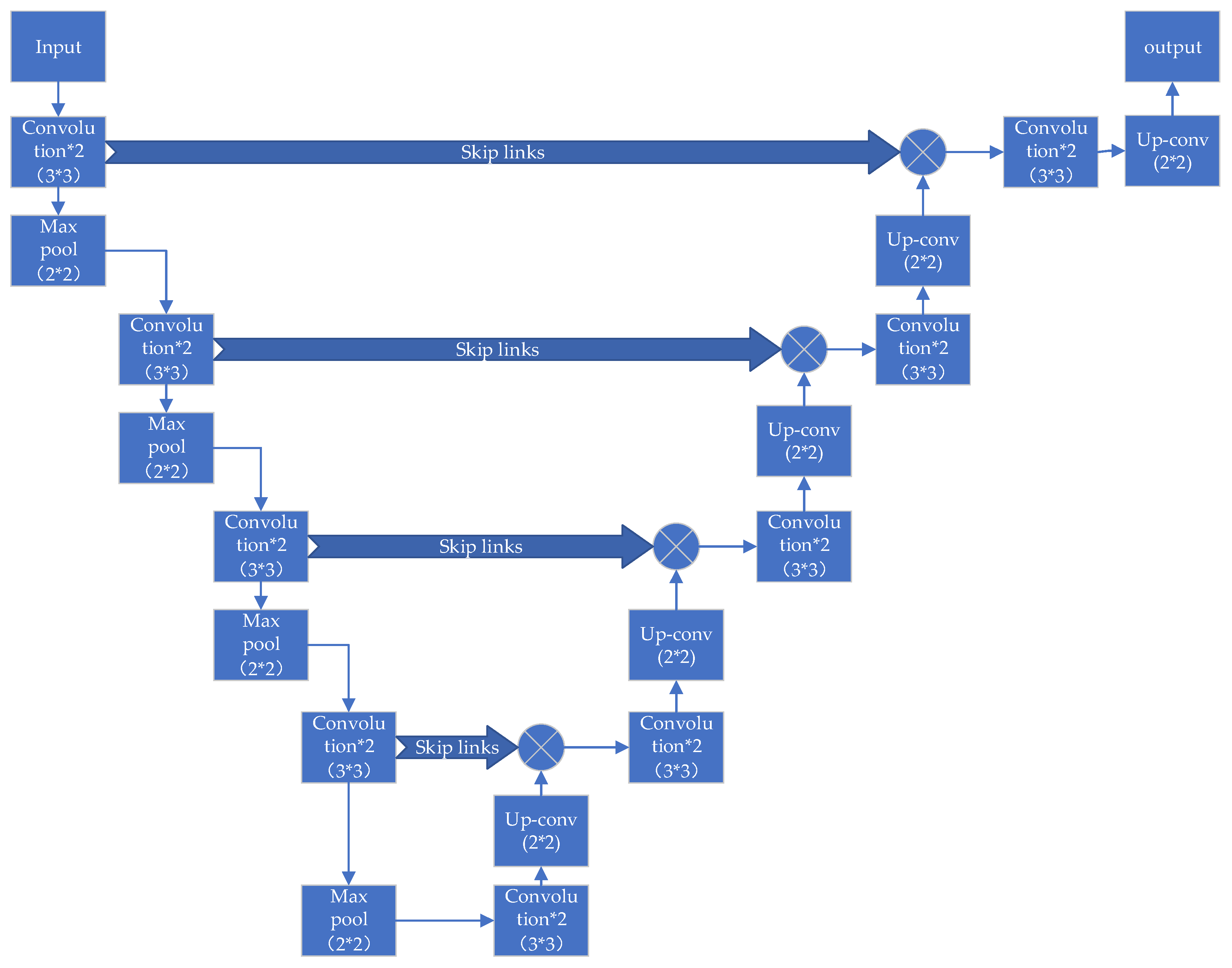
The convolutional neural network (CNN) is a neural network applied to image processing [39,40]. The low-level features are abstracted into high-level features through convolution so that the features of the image can be retained while a large number of parameters in the image data that are difficult to process can be reduced to a small number of parameters for further processing. The convolutional neural network performs layer-by-layer feature transformation on the input data, transforms the features of the samples in the original space to features in a new feature space, and learns in the new feature space to obtain a hierarchical feature representation, which can be used for classification or feature visualization. The convolutional neural network used for classification generally includes a convolutional layer, a pooling layer, and a fully connected layer [41,42,43]. The convolutional layer extracts local features in the image through the filtering of the convolution kernel; the pooling layer is the down-sampling layer, which is used to reduce the dimension of the data, reduce the number of calculations, and prevent overfitting; the fully connected layer is used for the output of classification results (see Figure 2).

It can be seen that this kind of network structure could achieve a high rate of accuracy in image recognition. However, it can only determine whether a certain feature is included in an image or not, but cannot identify information, such as the size and position of the feature, i.e., the image semantics are lost. The image prediction for land quality requires an end-to-end network structure to ensure that the output image should have the same scale as the input image.

Therefore, we will follow the process below (see Figure 3, Appendix B, and Appendix C) to train the CNN model, and get the final result.

Before data preprocessing, in order to prevent exploding gradients and avoid other problems in data processing, this paper has normalized the training set and labels:

$$u_{ij}=\frac{x_{ij}-g_{min}}{g_{max}-g_{min}}$$

(1)

where $u_{ij}$ is the normalized value; $x_{ij}$ is the grey value corresponding to each pixel; $g_{max}$ and $g_{min}$ represent the maximum and minimum values of the grey value, respectively. The grey value is the color depth of the points in the black and white image, ranging from 0 to 255. White is 255, and black is 0. The data obtained from images will automatically assign the color depth in ArcGIS 10.2 (the software of Environmental Systems Research Institute, Inc. Redlands, CA, USA), that is, the grey value, according to different land types.

In order to make the gradients calculated by the deep learning algorithm faster, the features are scaled to [0,1] on average, and the above work is completed by Equation (1). If the mean value is used, a large number of features will take a value close to 1 after calculation, making it difficult to calculate the gradients.

When inputting the data set, this paper performs feature transformation through convolution, i.e., following a u-net encoding process and performing convolution on a two-dimensional image. The convolution process can be expressed as:

$$h_{ij}={\displaystyle \sum }_{u=1}^m{\displaystyle \sum }_{v=1}^n{f}_{i-u+1,j-v+1}\times k_{uv}$$

(2)

where $f_{ij}$ is a given two-dimensional image and satisfies that $1\le i\le M$, $1\le j\le N$; $k_{uv}$ is the convolution kernel and satisfies that $1\le u\le m$, $1\le v\le n$.

The activation function $ReLU\left(x\right)$ (the Rectified Linear Unit) adopted in this paper is:

$$ReLU\left(x\right)=\{\begin{array}{c}x\left(x>0\right)\\ 0\left(x\le 0\right)\end{array}$$

(3)

Compared with the traditional activation function, this activation function can reduce the number of calculations, and increase the sparsity of the network by making some of the neuron outputs 0. In addition, this activation function can reduce the interdependence among parameters, thus, preventing “overfitting”, which refers to the phenomenon that the model has learned the training data so well that it even incorporates the potential noise in the training data so cannot recognize the data very well during actual testing, thus, impairing the model’s ability to generalize [44,45].

An initial value is assigned to the convolution kernel, and the He normal distribution initializer is applied here, which draws samples from a truncated normal distribution centered at 0 with a standard deviation of:

$$stddev=\sqrt{\frac{2}{fan\_in}}$$

(4)

in which $fan\_in$ is the number of input units in the weight tensor.

After the encoding is completed, this paper performs deconvolution (an inverse operation of convolution), i.e., interpreting the learned features through a u-net decoding process. Based on Formula (2), if * is used to denote convolution, the convolution process can be expressed as:

$$h=f\ast k$$

(5)

while the deconvolution process is to reconstruct $f$ when $h$ and $k$ are given.

The loss function is a product of the soft-max function and the cross-entropy. The soft-max function is defined as follows:

$$p_k\left(x\right)=\frac{exp\left(a_k\left(x\right)\right)}{{\sum }_{k^{\prime }}^{K}exp\left(a_{k^{\prime }}\left(x\right)\right)}$$

(6)

in which $a_k\left(x\right)$ represents the activation function of the feature channel k at the pixel position x. The loss function $E$ can be expressed as:

$$E={\displaystyle \sum }_{x\in \mathsf{\Omega }}w\left(x\right)log\left(p_{l\left(x\right)}\left(x\right)\right)$$

(7)

in which $w\left(x\right)$ is the weight introduced in this paper, which makes some features more important than others [46]. Here, the proportion of different terrains for map data from previous years are calculated, and corresponding weights are generated. For example, different weights are given to plain terrain and swamp terrain. In addition, additional weights are given to the boundaries of the classification features, such as the junction of marsh terrain and plain terrain. The network will minimize those additional weights to minimize the loss function $E$ and improve the accuracy of the classification boundaries.

In the image prediction of land quality, this paper has further adopted skip connections. Currently, as a common practice of CNN in the academic circle, the output of the previous layer is normally used as the input of the next layer, while skip connections mean connecting part of the output of the previous layer to a higher layer or more layers [47,48,49]. By using skip connections, the low-level features of an image can be fed to higher layers of the network to facilitate image prediction, while reducing the number of network parameters. According to the No Free Lunch (NFL) Theorem [50], the total error will not be impacted by the choice of machine learning algorithms, and the overall expected performance of any two algorithms is the same. Therefore, this paper has innovatively applied U-net to the image prediction task regarding land use.

More specifically, the network structure designed in this paper is u-net, which is symmetrical. The network on the left side is the encoder, i.e., the contracting path. The contracting path follows a typical convolutional network structure. The activation function $ReLU\left(x\right)$ is applied to the convolutional layer. The contracting path also includes a pooling operation with a step size of 2 to perform down-sampling in order to gradually reflect the environmental information regarding geographic locations in the contracting path. The network on the right is the decoder, i.e., the expanding path. Each step in the expanding path consists of the up-sampling information of the feature map and the down-sampling information from skip connections. These two types of information are combined to restore detailed information and gradually achieve image accuracy. The prediction results obtained through this method contain both information regarding geographic locations and detailed information about each location.

2.2. Data Sources and Data Processing Methods

The dataset used in this paper is the raster data per square kilometer of land in the Beijing-Tianjin-Hebei region of China from 1995 to 2018, collected by the Chinese Academy of Sciences [37]. In the dataset, different land types have been given different signs, which come with the raster data and follow the LUCC (Land Use Cover Change) classification system, which divides land types into six primary land types, and twenty-six secondary land types. The raster data can be displayed in color or greyscale [51]. In order to reduce the number of calculations, and reduce the errors caused by the transformation of colored images to greyscale images, this paper has used greyscale images to perform deep learning instead of transforming colored images to greyscale images.

The purpose of this paper is to make predictions on land types. Prediction is a classification task in itself. To train a neural network, it requires a given input and the corresponding results, which is the sign. Therefore, this paper has defined the input as the data of the n^th year, and defined the sign as the data after that year. The signs of different land types in different years are unique and consistent, which all come from the LUCC classification system. Because deep learning requires numerical values instead of signs, the signs are converted into grey values when performing deep learning, which ranges from 0 to 255, and distinguishes the features of different land types. Therefore, the range of [0,255] is divided into equal intervals, and each interval is used to represent a land type.

Because the remote sensing data is measured every five years, and thus, the data size is limited, this paper has expanded the data volume through data augmentation. The methods include expanding the data volume by image rotation, horizontal movement, vertical movement and horizontal flip while making the same adjustments to the image and the sign at the same time. In the data augmentation process, the input image is regarded as one channel, and the sign is regarded as another channel. The two channels are combined into one image and perform the same adjustments. After the data augmentation is completed, the image is split again to obtain the expanded dataset and signs.

Based on the above models and datasets, this paper has performed a trend forecast of land types in the Beijing-Tianjin-Hebei region in 2023. The trend prediction map includes both changes in the grey values that match the existing grey values and grey values that do not match the existing grey values. By comparing the trend prediction map with the sample, this paper has obtained a land type map reflecting the detailed future changes in the land resources of the Beijing-Tianjin-Hebei region. The following formula was used to calculate the percentage change of land types:

$$P_n=A_n/S_n-A_{n-1}/S_{n-1}$$

(8)

in which n is the label of the data set; $P_n$ is the percentage change of the corresponding land type; $A_n$ is the area of the corresponding land type in the dataset; $S_n$ is the total area of the land; $A_{n-1}$ is the area of the corresponding land type in the previous period; and $S_{n-1}$ is the total area of the land in the previous period.

The calculation software used in this paper is Python 3.7.6 by Python Software Foundation (Beaverton, OR, USA). The training code and the trend forecast code of CNN model are listed in Appendix B and Appendix C.

3. Results

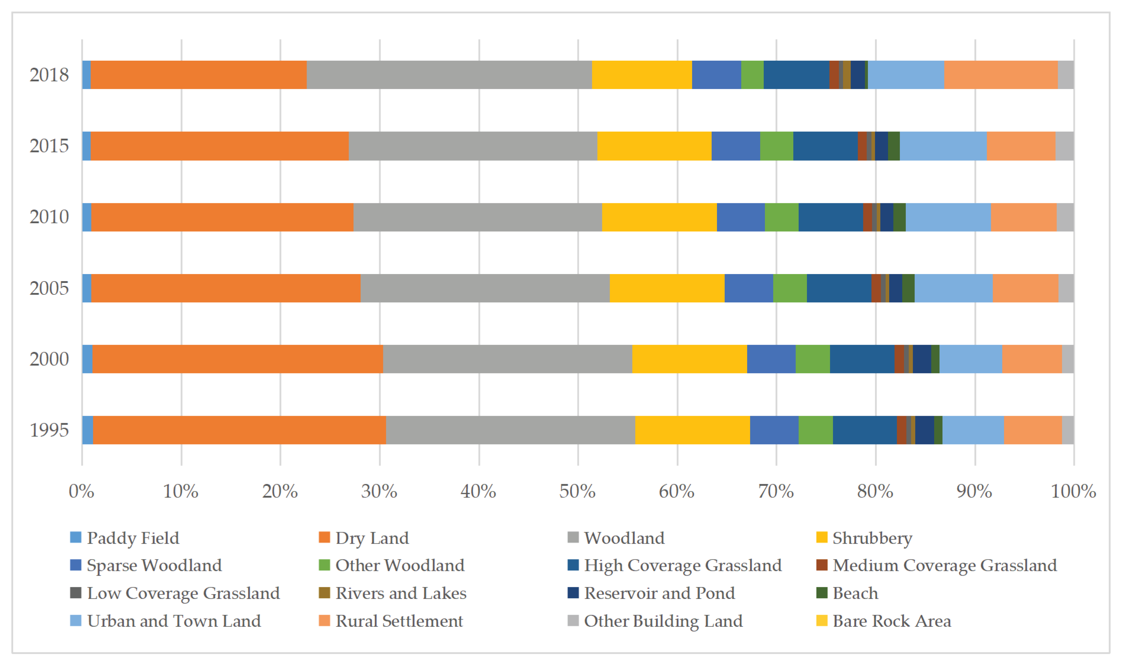
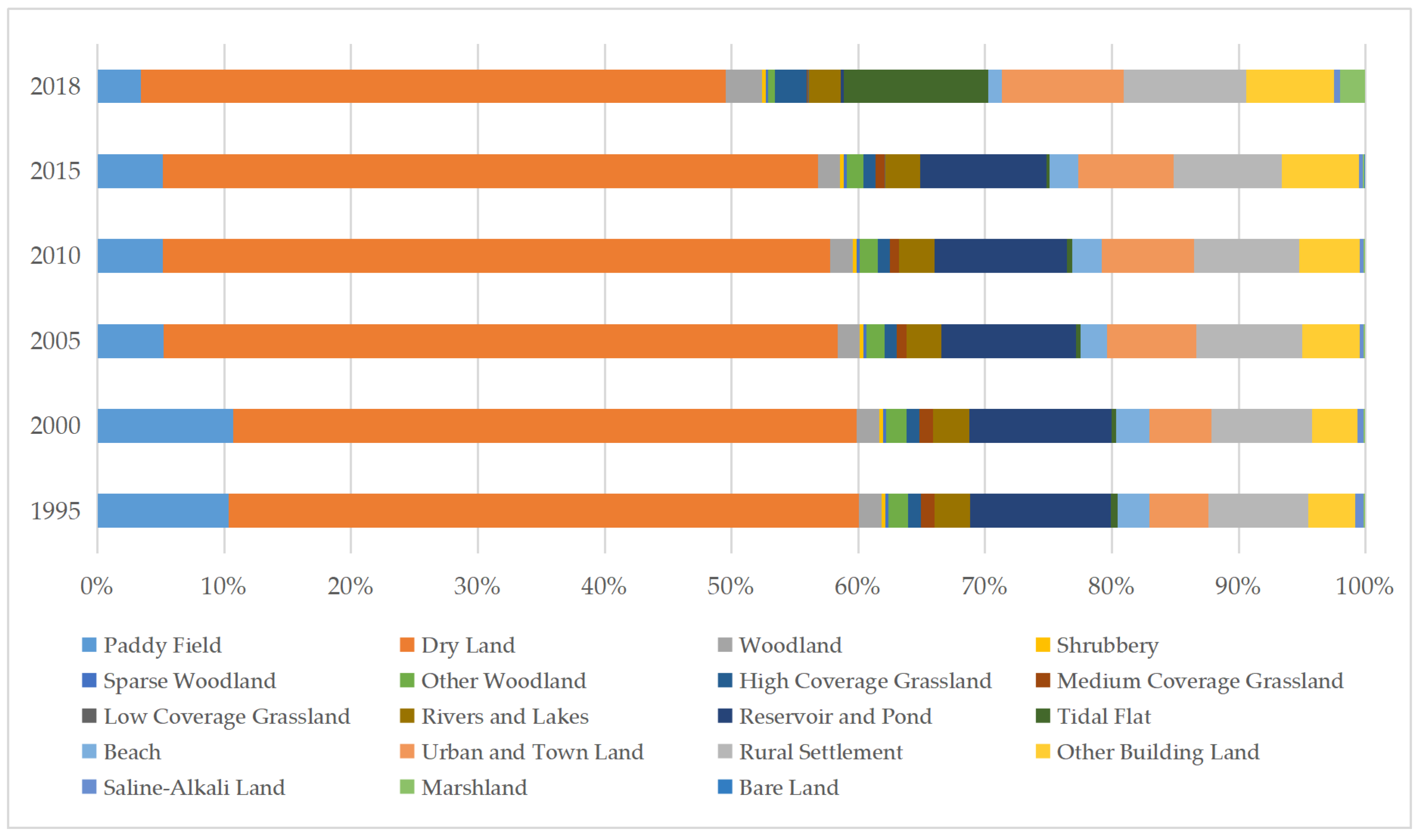
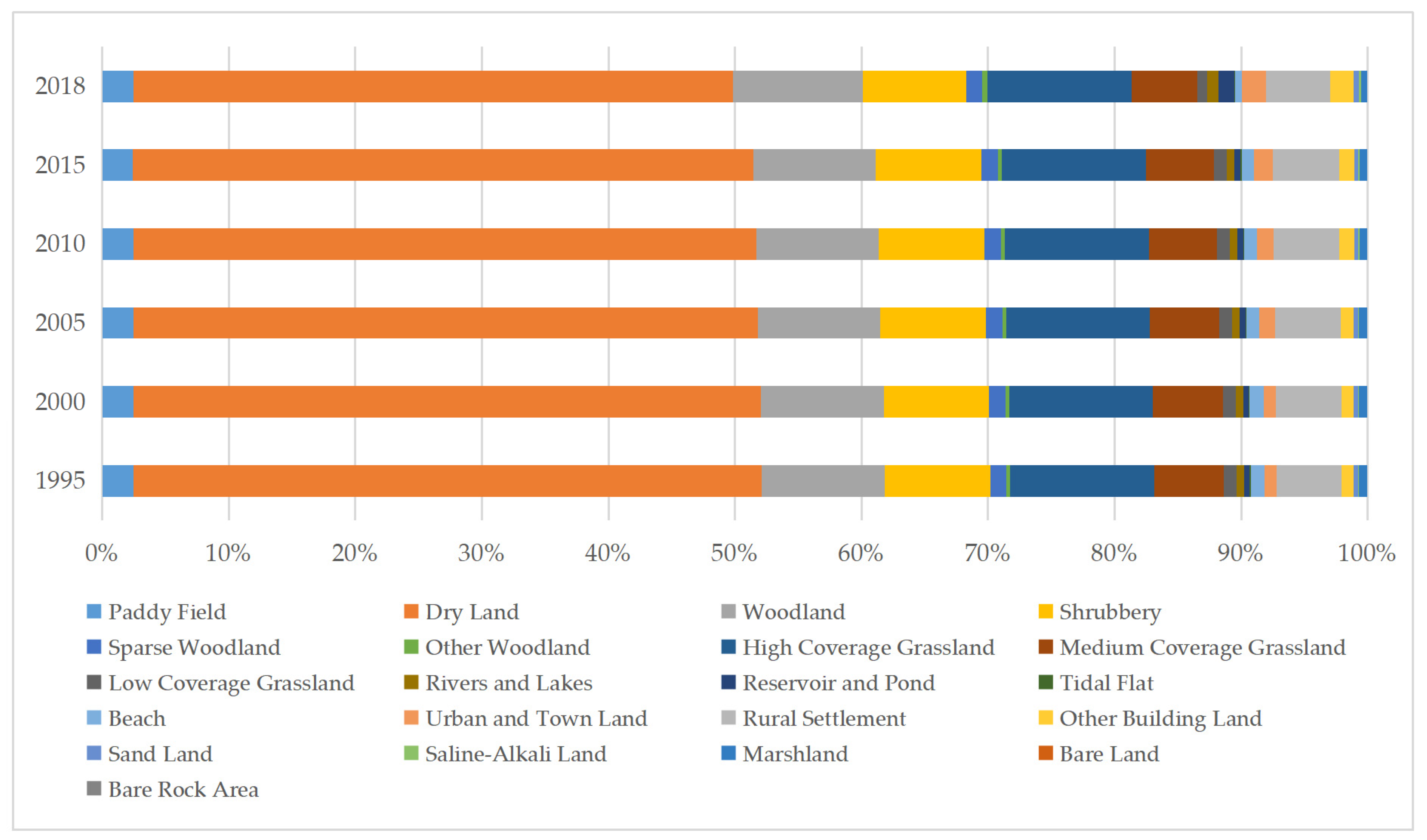
Based on the model and data introduced in Part 2, this paper has calculated the proportion of various land types in the Beijing-Tianjin-Hebei region from 1995 to 2018, as shown in Figure 4, Figure 5 and Figure 6, and

Table A1. The proportion of various land types in Beijing from 1995 to 2018.

	1995	2000	2005	2010	2015	2018
Paddy Field	1.07%	1.04%	0.93%	0.89%	0.85%	0.86%
Dry Land	29.55%	29.31%	27.14%	26.45%	26.01%	21.79%
Woodland	25.10%	25.09%	25.09%	25.06%	25.05%	28.71%
Shrubbery	11.60%	11.59%	11.59%	11.57%	11.55%	10.09%
Sparse Woodland	4.89%	4.89%	4.87%	4.85%	4.85%	4.99%
Other Woodland	3.48%	3.48%	3.45%	3.41%	3.39%	2.24%
High Coverage Grassland	6.43%	6.46%	6.48%	6.46%	6.45%	6.61%
Medium Coverage Grassland	0.96%	0.96%	0.96%	0.94%	0.94%	1.00%
Low Coverage Grassland	0.49%	0.47%	0.45%	0.44%	0.44%	0.42%
Rivers and Lakes	0.41%	0.41%	0.39%	0.40%	0.40%	0.73%
Reservoir and Pond	1.87%	1.85%	1.31%	1.31%	1.29%	1.47%
Beach	0.86%	0.87%	1.26%	1.21%	1.21%	0.29%
Urban and Town Land	6.23%	6.34%	7.88%	8.63%	8.75%	7.68%
Rural Settlement	5.83%	5.97%	6.62%	6.62%	6.91%	11.46%
Other Building Land	1.22%	1.26%	1.57%	1.75%	1.90%	1.65%
Bare Rock Area	0.01%	0.01%	0.01%	0.01%	0.01%	0.01%

,

Table A2. The proportion of various land types in Tianjin from 1995 to 2018.

	1995	2000	2005	2010	2015	2018
Paddy Field	10.35%	10.71%	5.24%	5.18%	5.17%	3.41%
Dry Land	49.66%	49.13%	53.10%	52.61%	51.62%	46.15%
Woodland	1.81%	1.81%	1.77%	1.76%	1.74%	2.85%
Shrubbery	0.31%	0.31%	0.31%	0.31%	0.31%	0.29%
Sparse Woodland	0.22%	0.22%	0.22%	0.22%	0.22%	0.17%
Other Woodland	1.59%	1.60%	1.43%	1.43%	1.36%	0.55%
High Coverage Grassland	1.00%	1.04%	0.98%	0.98%	0.96%	2.50%
Medium Coverage Grassland	1.04%	1.04%	0.72%	0.71%	0.71%	0.07%
Low Coverage Grassland	0.02%	0.02%	0.02%	0.02%	0.03%	0.10%
Rivers and Lakes	2.82%	2.87%	2.77%	2.77%	2.77%	2.50%
Reservoir and Pond	11.10%	11.23%	10.63%	10.45%	9.95%	0.23%
Tidal Flat	0.50%	0.34%	0.34%	0.40%	0.22%	11.45%
Beach	2.53%	2.65%	2.09%	2.33%	2.31%	1.02%
Urban and Town Land	4.66%	4.89%	7.05%	7.29%	7.49%	9.60%
Rural Settlement	7.87%	7.91%	8.33%	8.33%	8.53%	9.72%
Other Building Land	3.67%	3.58%	4.52%	4.75%	6.09%	6.91%
Saline-Alkali Land	0.67%	0.47%	0.34%	0.32%	0.29%	0.45%
Marshland	0.17%	0.17%	0.13%	0.13%	0.13%	1.98%
Bare Land	0.01%	0.01%	0.01%	0.01%	0.10%	0.05%

and

Table A3. The proportion of various land types in Hebei province from 1995 to 2018.

	1995	2000	2005	2010	2015	2018
Paddy Field	2.49%	2.49%	2.46%	2.44%	2.41%	2.49%
Dry Land	49.62%	49.58%	49.37%	49.24%	49.05%	47.37%
Woodland	9.71%	9.67%	9.67%	9.68%	9.67%	10.21%
Shrubbery	8.34%	8.35%	8.34%	8.34%	8.34%	8.19%
Sparse Woodland	1.30%	1.30%	1.29%	1.29%	1.31%	1.27%
Other Woodland	0.30%	0.29%	0.32%	0.32%	0.32%	0.43%
High Coverage Grassland	11.34%	11.35%	11.31%	11.38%	11.37%	11.40%
Medium Coverage Grassland	5.51%	5.50%	5.48%	5.38%	5.38%	5.14%
Low Coverage Grassland	1.04%	1.04%	1.03%	1.02%	1.02%	0.83%
Rivers and Lakes	0.59%	0.59%	0.57%	0.58%	0.58%	0.86%
Reservoir and Pond	0.42%	0.41%	0.48%	0.47%	0.50%	1.25%
Tidal Flat	0.11%	0.10%	0.08%	0.08%	0.07%	0.10%
Beach	1.05%	1.09%	1.03%	1.01%	1.01%	0.51%
Urban and Town Land	0.95%	0.98%	1.22%	1.31%	1.44%	1.91%
Rural Settlement	5.16%	5.18%	5.20%	5.23%	5.26%	5.07%
Other Building Land	0.93%	0.94%	1.05%	1.14%	1.19%	1.86%
Sand Land	0.37%	0.37%	0.35%	0.34%	0.34%	0.43%
Saline-Alkali Land	0.08%	0.08%	0.07%	0.08%	0.08%	0.17%
Marshland	0.64%	0.64%	0.63%	0.62%	0.61%	0.46%
Bare Land	0.02%	0.02%	0.02%	0.02%	0.02%	0.02%
Bare Rock Area	0.03%	0.03%	0.03%	0.03%	0.03%	0.03%

in Appendix A.

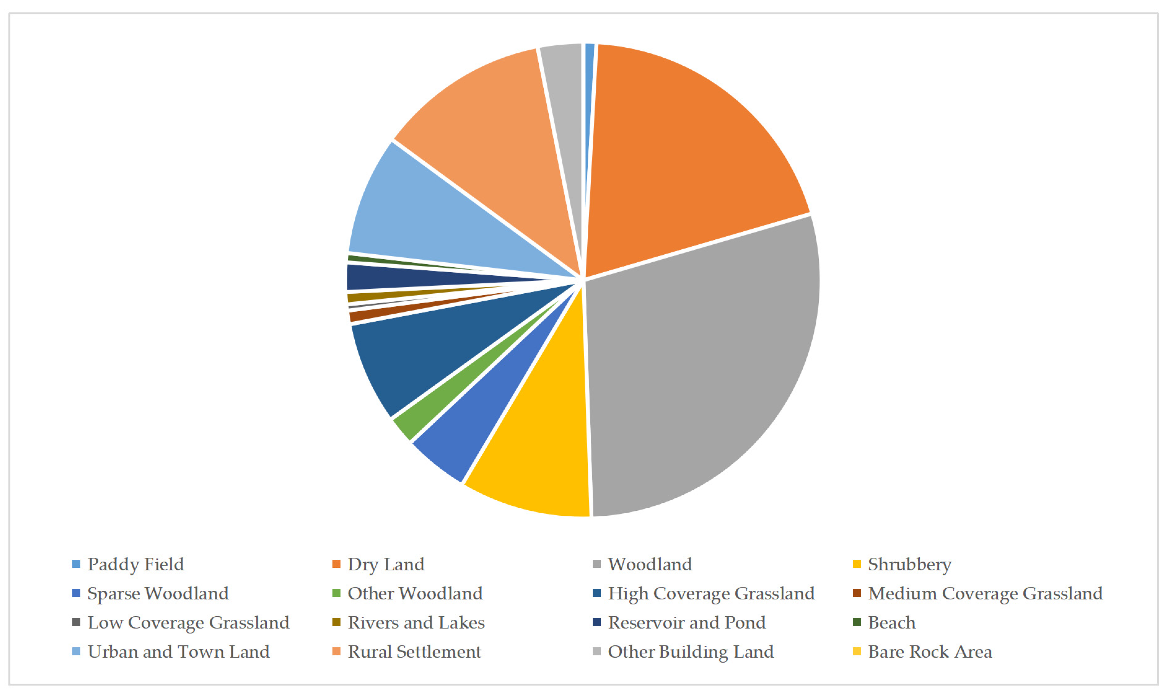
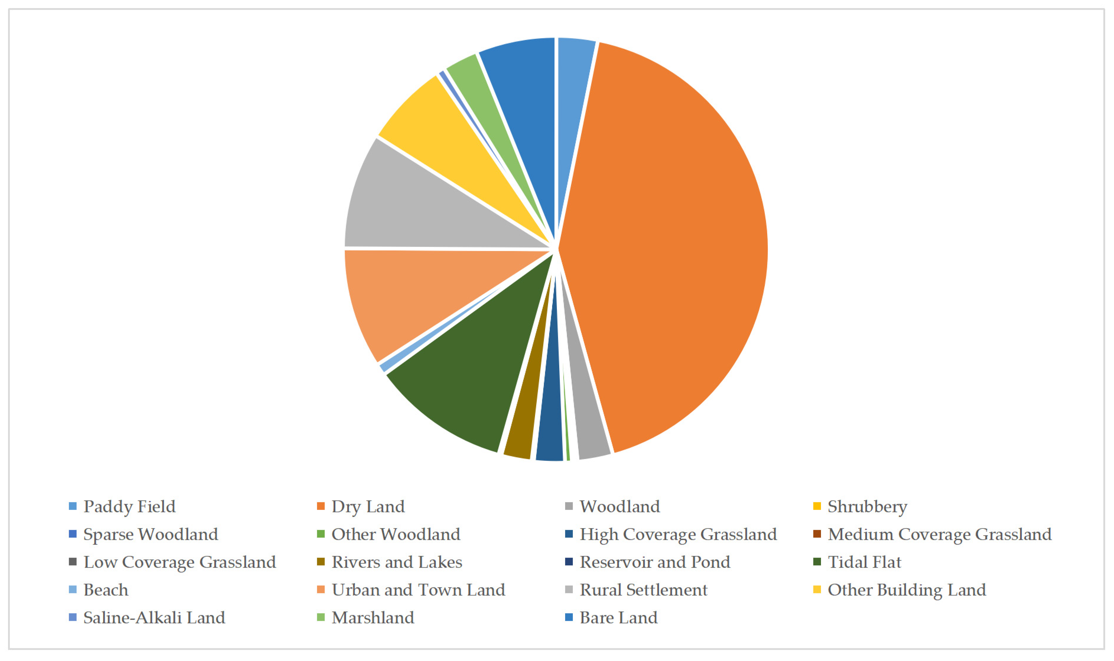
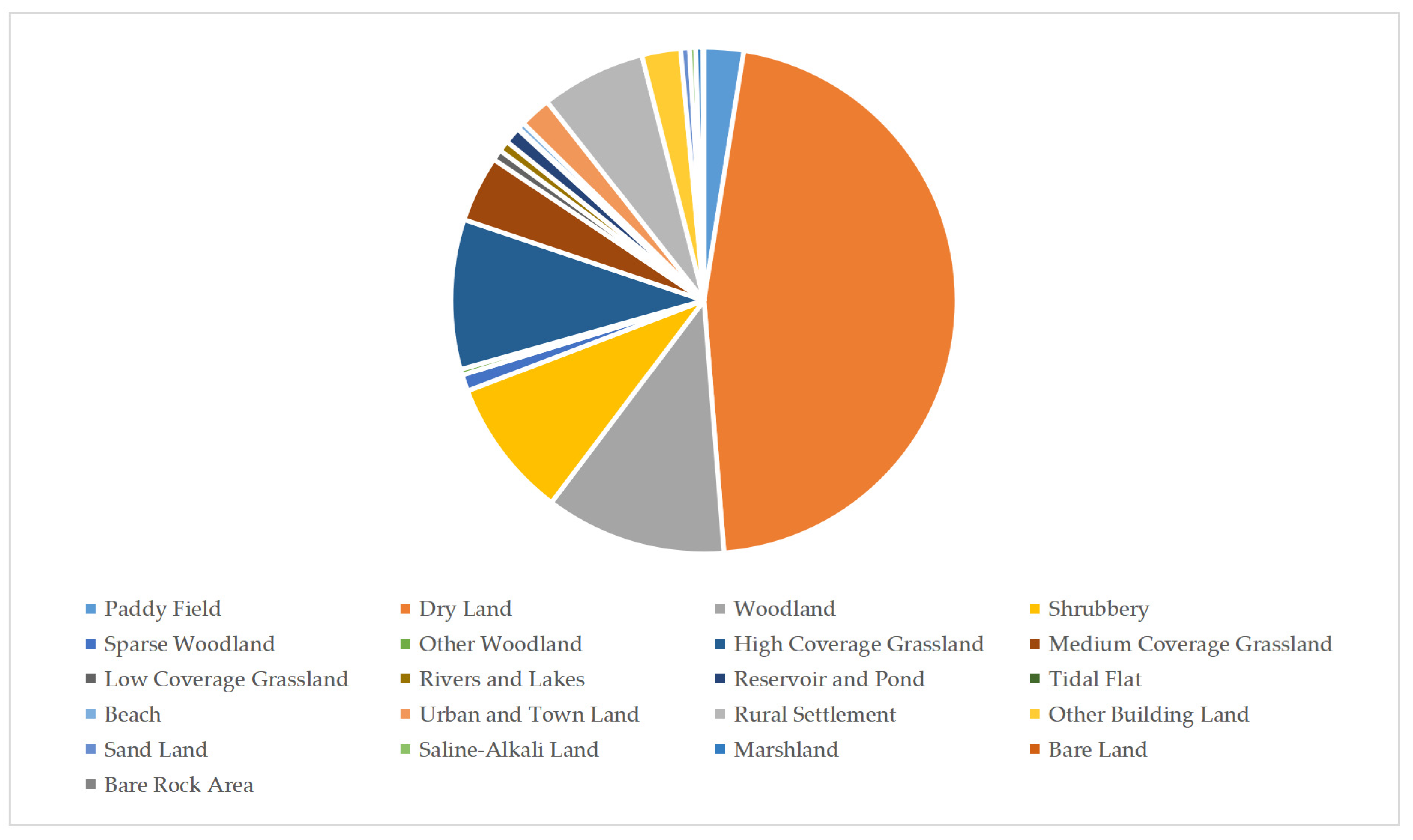
Further, this paper has predicted the proportion of various land types in the Beijing-Tianjin-Hebei region in 2023. The prediction result is shown in Figure 7, Figure 8 and Figure 9, and

Table A4. The predicted proportions of various land types in the Beijing-Tianjin-Hebei region in 2023.

	Beijing	Tianjin	Hebei
Paddy Field	0.88%	3.14%	2.52%
Dry Land	19.61%	42.57%	46.22%
Woodland	28.97%	2.69%	11.55%
Shrubbery	9.07%	0.27%	8.89%
Sparse Woodland	4.48%	0.16%	1.06%
Other Woodland	2.04%	0.52%	0.37%
High Coverage Grassland	6.99%	2.34%	9.56%
Medium Coverage Grassland	0.92%	0.06%	4.24%
Low Coverage Grassland	0.42%	0.10%	0.69%
Rivers and Lakes	0.83%	2.31%	0.70%
Reservoir and Pond	1.99%	0.21%	1.04%
Tidal Flat	/	10.64%	0.08%
Beach	0.63%	0.89%	0.43%
Urban and Town Land	8.25%	9.18%	2.01%
Rural Settlement	11.83%	8.87%	6.69%
Other Building Land	3.08%	6.55%	2.47%
Sand Land	/	/	0.56%
Saline-Alkali Land	/	0.66%	0.39%
Marshland	/	2.73%	0.46%
Bare Land	/	6.11%	0.03%
Bare Rock Area	0.01%	/	0.04%

in Appendix A.

4. Discussion

As the above calculation results show, land resource sustainability in the Beijing-Tianjin-Hebei region is not optimistic. In 1995, dry land took up the largest proportion in Beijing, Tianjin, and Hebei, with a proportion of 29.55%, 49.66%, and 49.62%, respectively. In 2018, the land type that took up the largest proportion in Beijing changed to woodland, accounting for 28.71% of the total land area; while the land type that occupied the largest proportion of land area in Tianjin and Hebei was still dry land, with a proportion of 46.15% and 47.37%, respectively. The area of dry land in these three locations all decreased compared with that of 1995, with Beijing witnessing the largest decline. Due to the continuous development of urban areas, the proportions of residential land and building land have shown an increasing trend in Beijing, Tianjin, and Hebei. However, the large proportion of dry land indicates that there is still much room for land resource utilization within these three locations.

4.1. Beijing

The prediction results show that in 2023, the proportion of woodland in Beijing would increase by 0.26%, compared with that in 2018, and increase by 3.92%, compared with that in 2015—reaching its best level since 1995. Meanwhile, in 2023, the proportion of grasslands (including high-, medium-, and low-coverage grassland) in Beijing would increase by 0.30%, compared with that in 2018, and increase by 0.50%, compared with that in 2015; while the total proportion of rivers, lakes, reservoirs, and ponds would increase by 0.61%, compared with that in 2018, and increase by 1.13%, compared with that in 2015—also reaching its best level since 1995. The increase in the proportions of the above three land types indicates that Beijing has attached importance to ecological environment protection when pursuing socio-economic development. This also indicates that Beijing’s land resources have been well protected.

During the research period of this paper, Beijing has adopted a number of policies and measures to protect the ecological environment and reasonably utilize and develop its land resources. In 2009, Beijing published the “Beijing Master Plan for Land Use (2006–2020)”, establishing the guiding principle of “emphasizing ecological civilization, and promoting reasonable utilization and optimized allocation of land resources” for land use in the next 15 years [52]. This plan has been the mandatory general policy for land use in Beijing since 2009. Governments at all levels in Beijing have strictly adhered to the requirements of it. Taking green space protection and construction as an example, the plan requires the construction of a “three green circles” urban land use pattern in Beijing. That is to build three green ecological areas: (1) The core area of urban greening—the area between the first greenbelt and the second greenbelt around the city; (2) plain farmland ecosphere—a concentrated distribution area of nine planned basic green farmlands in the suburbs; (3) mountain ecological circle—the area around the Yanshan and Taihang Mountains [52].

The calculation results in this paper fully show the effect of the above plan. The proportion of woodland and grassland area in Beijing in 2018 increased significantly compared to 2005—the woodland coverage increased from 45.00% in 2005 to 46.03% in 2018, and the grassland coverage increased from 7.89% in 2005 to 8.03% in 2018. Based on Beijing’s total area of 16,410 square kilometers [38], the woodland and grassland increased by 169.02 square kilometers and 22.97 square kilometers, respectively.

In the above calculation process, the machine learning processes during CNN model application fully considered and reflected the effect of policies on land change. In the data, the color patches of the grey values corresponding to the woodland and grassland types increased significantly. In the algorithm, the CNN model can be understood as each class of features is extracted. For example, the first layer of convolution may extract features of the terrain contours, and the second layer extracts these contour features to acquire the deep-level features, such as which types of land are more likely to change into woodland and grassland during the implementation of the policy. The more abstract the feature, the more convolution operations need to be performed, and the deeper the level. The change in the above policy causes a sudden increase in the change of a certain land type, which can be extracted by the deeper convolution layer to reflect, so that the final forecast result can further reflect the future impact of the policy.

In the actual operation, the convolution layer of the model performs the convolution operation according to the type of color patch. The shallow convolution operation extracts the geographical location where the color patch changes more. The deep convolution operation is based on the shallow layer and combines the features of the shallow operation to extract features—such as the trend of the policy—to fit the effect of it, so that the final prediction result can fully reflect the role of policy.

In 2017, Beijing further formulated the “Guidelines for Beijing Urban and Rural Planning and Land Use Type Classification (Trial)”, which have matches Beijing’s current land type classification in urban and rural planning, as well as land classification standards with the national land standards of China, in order to ensure the reasonable and efficient utilization [53].

These policies have played a positive role in Beijing’s development of land resources and contributed to the protection and restoration of its ecological environment. The proportions of urban woodland and grassland have shown an increasing trend. The proportion of woodland increased from 25.05%, in 2015, to 28.71%, in 2018 (an increase of 3.65%); and among the various types of grasslands, the growth in high coverage grassland is the most prominent—where the proportion of total land area increased from 6.45% to 6.61% (an increase of 0.15%). The increase in the proportions of woodland and high coverage grassland could help reduce the carbon dioxide content in the atmosphere and lessen the greenhouse effect, which also plays a role in air purification and climate adjustment, and helps alleviate the pressure on the environment brought by the continuous development and increasingly concentrated population of Beijing [54,55,56,57]. In addition, the proportion of rivers and lakes, as well as that of reservoirs and ponds, have also increased in Beijing—increasing by 0.34% and 0.18%, respectively, in 2018, compared to figures from 2015.

4.2. Tianjin

During the research period, the land use type in Tianjin was generally stable. Although the area of dry land is still quite large, the proportions of woodland and grassland have both increased while ensuring the development of building lands. In 2018, the proportion of woodland in Tianjin was 2.85%, increasing by 1.04% compared with that in 1995; while the proportion of grassland (including high-, medium-, and low-coverage grassland) was 2.67%, increasing by 0.61% compared with that in 1995.

Since 2010, Tianjin has formulated and implemented a series of land-use-related measures for ecological environment management based on China’s overall policy regarding the construction of ecological civilization. For example, the “Tianjin Master Plan for Land Use (2006–2020)” was published in 2010 [58], and the “Regulations on the Management of Tianjin’s Permanent Ecological Protection Areas” and their revised editions were issued in 2014 [59] and 2019 [60], respectively. Tianjin has made concentrated efforts to solve the remaining issues in the ecological environment generated in the process of urban construction and land development. Tianjin has also taken the lead in the country by designating permanent ecological protection areas through local legislation, including six types of areas (mountains, rivers, reservoirs and lakes, wetlands and salt fields, country parks and urban parks, and forest belts) into the scope of permanent protection. At the same time, Tianjin has further increased its efforts in tree planting and afforestation, and has implemented key national projects, such as the control of sources of sandstorms in Beijing and Tianjin, and the construction of the northwest–north–northeast shelter forest and the coastal shelter forest. According to the statistics in the “Thirteenth Five-Year Plan for Ecological Environmental Protection of Tianjin”, from 2011 to 2015, Tianjin has completed a total forest plantation of 1.554 million mu, promoted afforestation and beautification campaigns, and constructed a few new country parks, including Xiqing, Dongli, Jinnan, and Guangang Country Park of Binhai New Area [61].

In addition, Tianjin has also vigorously implemented construction projects—such as wetland protection and restoration, sandstorm prevention and control, mine management, and small watershed cleansing. Within the research period, Tianjin has constructed two national-level wetland parks, and actively carried out pilot programs on soil erosion control in the plain area. Through afforestation and cultivation measures on the desertified land in the city, Tianjin has effectively controlled land desertification. At the same time, Tianjin has also enhanced soil environment protection by setting up 195 control points all over the city for soil environment quality monitoring, and establishing a city-wide network that monitors the quality of the soil environment [61]. With the help of this monitoring network, Tianjin has carried out a detailed investigation on the status of closed industrial enterprises and their development and utilization of land, thus, providing a scientific basis for the environmental risk assessment of the reuse of contaminated sites.

The above policies have achieved positive results. By 2018, with increasing proportions of woodland and grassland in Tianjin, the proportion of saline-alkali land has also decreased by 0.22% since the beginning period of 1995, which has effectively promoted the efficient use of land resources in Tianjin. The Saline-alkali land is one of the main obstacles affecting the ecological environment of Tianjin. Based on Tianjin’s total area of 11,966 square kilometers [38], it is equivalent to adding 26.33 square kilometers of land for being improved to woodland and grassland, and for urban construction. Therefore, it has played a positive role in improving the air quality and protecting the ecological environment in Tianjin in recent years.

4.3. Hebei

The prediction results of Hebei for 2023 have clearly reflected the ecological and environmental problems brought by the previous highway construction. The area of building land has been expanding day by day, and the area of sand land, saline-alkali land, marshland, bare land and bare rock area has also increased at the same time. In 2018, the total proportion of Hebei’s urban and town land, rural settlement and other building land was 8.84%, which is an increase of 1.80% compared with that of 1995, and is predicted to further increase to 11.17% by 2023. Its total proportion of sand land, saline-alkali land, marshland, bare land and bare rock area is predicted to reach 1.48% by 2023, increasing by 0.34% compared with that of 1995.

Facing the adverse situation, Hebei has also formulated a number of policies to promote proper utilization and protection of land resources. Based on the 1.415 million mu of newly constructed building land during the “Twelfth Five-Year Plan” period, in 2017, Hebei issued the “Thirteenth Five-Year Plan for Land and Resources in Hebei Province”, which calls for strong support to the land needs of new industries and new business forms, as well as an effective guarantee of land resources required by the sustainable socio-economic development of Hebei Province [62]. For this purpose, Hebei Province has planned its land development and construction of ecological civilization as a whole, and prioritized ecological environment protection during land development to prevent excessive development and predatory use of land, and to ensure that the development of land does not exceed the carrying capacity of resources and the environment. At the same time, Hebei Province has also strengthened land-related ecological environmental protection and comprehensive improvement, emphasized source protection and restoration of ecological functions, and promoted reduced development, intensive development and renewable development to continuously advance the construction of an ecological land.

On the other hand, Hebei has also attached great importance to the protection and improvement of its river, lake, reservoir, and pond resources. Hebei has focused on the treatment of water pollution in the water sources of its drinking water, as well as the Haihe River basin, designated key control areas in cities under its jurisdiction, and made concentrated efforts in the pollution rectification and prevention of rivers, lakes, reservoirs and ponds. The above policies have achieved some results. In 2018, the total proportion of rivers, lakes, reservoirs and ponds in Hebei Province reached 2.11%, increasing by 1.10% compared with that of 1995. At the same time, the comprehensive water network management capacity of Hebei has enhanced, and Hebei’s water quality has seen significant improvements.

4.4. Overview of the Whole Region

In summary, the land use situation in the Beijing-Tianjin-Hebei region has not reached the ideal state. By 2018, the proportion of dry land in the entire region is still high, especially in Tianjin and Hebei. Although the dry land in Tianjin dropped from more than 50% in 2005–2015 to 46.15% in 2018, the task of rebuilding dry land is still arduous. While a large area of dry land in this region is related to natural and climatic conditions [63], it is concerning that there is almost no special policy for dry land management in the land use policies in the Beijing-Tianjin-Hebei region—this is also an important reason for the high proportion of dry land there.

Another important trend is that construction land in the region (including Urban and Town Land, Rural Settlement, and Other Building Land) grew rapidly during the study period, and fully matched the level of urbanization and economic development. In 1995, the proportion of construction land in Beijing, Tianjin, and Hebei was 13.28%, 16.20%, and 7.04%, respectively. In 2018, the proportion increased in the three places to 20.79%, 26.23%, and 8.84%. As the capital of China, Beijing has always strictly controlled the rate of population growth and urbanization [64]. Therefore, the growth rate of its construction land is lower than that of Tianjin, and the relative backwardness of Hebei in the Beijing-Tianjin-Hebei region [38] has also been proven in the growth rate of construction land.

Based on the calculation results of 1995–2018, predictions on the land use status of Beijing-Tianjin-Hebei region in 2023 show that the construction land in the area will further increase with economic development. However, if land resources, such as the dry land, are not fully utilized, the proportion of woodland and grassland area may be further reduced. The forecast results for Beijing show that the proportion of woodland and grassland area in 2023 will be 52.89%, which will be 1.17% lower than 2018. Therefore, Beijing, and the entire Beijing-Tianjin-Hebei region, need to further consolidate the achievements of greening and environmental protection, so as to strengthen the rational use of land resources while maintaining sound economic development.

Due to data limitations, there may be some uncertainty in the results of calculations and analysis in this paper—the Chinese Academy of Sciences generally publish them on a 5-year cycle, not every year [37]. Therefore, the calculation and forecast results in this article are based on the time of publication. Considering that the period of land planning and urban construction is relatively long [65], and that China has always been making its development plan on a five-year cycle [66], this uncertainty is only likely to affect the land use analysis for each year in future researches, while not affect the results of this paper.

5. Conclusions

By using an improved CCN model, this paper has analyzed the land use of the Beijing-Tianjin-Hebei region of China from 1995 to 2018, and performed prediction for 2023. The research results show that: (1) There is still much room for improvement in the land use of the Beijing-Tianjin-Hebei region. In 1995, dry land took up the largest proportion of land in these three locations, with a proportion of 29.55%, 49.66%, and 49.62%, respectively. In 2018, the land type that took up the largest proportion in Beijing changed to woodland, accounting for 28.71% of the total land area; while the land type that occupied the largest proportion of land area in Tianjin and Hebei was still dry land, with a proportion of 46.15% and 47.37%, respectively. (2) Beijing’s land resources have been well protected in terms of land use. It is predicted that by 2023, the proportions of its woodland, grassland, and rivers, lakes, reservoirs and ponds would increase by 0.26%, 0.30%, and 0.61%, respectively compared with their proportion in 2018, reaching its best level since 1995. (3) The land use type in Tianjin during the research period was generally stable. In 2018, the proportion of its woodland and grassland had increased by 1.04% and 0.61%, respectively, compared with that of 1995. (4) Many ecological and environmental problems were exposed during the construction of highways in Hebei province. The proportions of its sand land, saline-alkali land, marshland, bare land, and bare rock areas have all increased, and their total proportion is predicted to reach 1.48% by 2023, increasing by 0.34% compared with that of 1995.

In summary, the land use situation in the Beijing-Tianjin-Hebei region has not reached the ideal state. By 2018, the proportion of dry land in the entire region is still high, especially in Tianjin and Hebei. Although the dry land in Tianjin dropped from more than 50% between 2005–2015, to 46.15% in 2018, the task of rebuilding dry land is still arduous. Another important trend is that construction land in the region (including Urban and Town Land, Rural Settlement, and Other Building Land) grew rapidly during the study period, and fully matched the level of urbanization and economic development. Based on the calculation results of 1995–2018, predictions on the land use status of Beijing-Tianjin-Hebei region in 2023 show that the construction land in the area will further increase with economic development. However, if land resources, such as the dry land, are not fully utilized, the proportion of woodland and grassland area may be further reduced.

Based on the above research findings, this paper has proposed the following policy recommendations for the land use in the Beijing-Tianjin-Hebei region:

(1) Attach equal importance to economic development and ecological protection. Take environmental protection and ecological enhancement into consideration when developing land resources for economic construction, and adhered to a strategy of sustainable development. Hebei can learn from the various measures in the land planning of Beijing and Tianjin, such as the measures in the “Guidelines for Beijing Urban and Rural Planning and Land Use Type Classification (Trial)” [53], and the “Regulations on the Management of Tianjin’s Permanent Ecological Protection Areas” [60], in order to match Hebei’s current land type classification in urban and rural planning, as well as land classification standards with the national land standards of China, and ensure the reasonable and efficient utilization.

(2) In the background of Beijing-Tianjin-Hebei integration, these three cities and provinces should coordinate the formulation and implementation of their land resource planning, realize comprehensive development and utilization of land resources in this region. In principle, no new construction land will be arranged, and the conversion of existing construction land into ecological land will be encouraged. However, high-intensity large-scale construction should not be carried out in the stock-excavation area. The total area of construction land will remain basically stable [67].

References

1. World Commission on Environment and Development. Our Common Future; Oxford University Press: Oxford, UK, 1987. [Google Scholar]
2. Yang, W.; Li, L. Energy Efficiency, Ownership Structure, and Sustainable Development: Evidence from China. Sustainability 2017, 9, 912. [Google Scholar] [CrossRef] [Green Version]
3. Jónsson, J.; Davíðsdóttir, B.; Jónsdóttir, E.M.; Kristinsdóttir, S.M.; Ragnarsdóttir, K.V. Soil indicators for sustainable development: A transdisciplinary approach for indicator development using expert stakeholders. Agric. Ecosyst. Environ. 2016, 232, 179–189. [Google Scholar] [CrossRef]
4. Edrisi, S.; Tripathi, V. Managing soil resources for sustainable development. J. Clean. Prod. 2018, 174, 199–200. [Google Scholar] [CrossRef]
5. Asimeh, M.; Nooripoor, M.; Azadi, H.; Van Eetvelde, V.; Sklenička, P.; Witlox, F. Agricultural land use sustainability in Southwest Iran: Improving land leveling using consolidation plans. Land Use Policy 2020, 94, 104555. [Google Scholar] [CrossRef]
6. Yang, W.; Li, L. Efficiency evaluation of industrial waste gas control in China: A study based on data envelopment analysis (DEA) model. J. Clean. Prod. 2018, 179, 1–11. [Google Scholar] [CrossRef]
7. Khantachavana, S.V.; Turvey, C.; Kong, R.; Xia, X. On the transaction values of land use rights in rural China. J. Comp. Econ. 2013, 41, 863–878. [Google Scholar] [CrossRef]
8. Zoomers, A.; Van Noorloos, F.; Otsuki, K.; Steel, G.; Van Westen, G. The Rush for Land in an Urbanizing World: From Land Grabbing Toward Developing Safe, Resilient, and Sustainable Cities and Landscapes. World Dev. 2017, 92, 242–252. [Google Scholar] [CrossRef]
9. Shen, X.; Yang, W.; Sun, S.; Sun, A.S. Analysis of the Impact of China’s Hierarchical Medical System and Online Appointment Diagnosis System on the Sustainable Development of Public Health: A Case Study of Shanghai. Sustainability 2019, 11, 6564. [Google Scholar] [CrossRef] [Green Version]
10. Mertz, O.; Mertens, C.F. Land Sparing and Land Sharing Policies in Developing Countries – Drivers and Linkages to Scientific Debates. World Dev. 2017, 98, 523–535. [Google Scholar] [CrossRef]
11. Reidsma, P.; Feng, S.; Van Loon, M.; Luo, X.; Kang, C.; Lubbers, M.; Kanellopoulos, A.; Wolf, J.; Van Ittersum, M.; Qu, F. Integrated assessment of agricultural land use policies on nutrient pollution and sustainable development in Taihu Basin, China. Environ. Sci. Policy 2012, 18, 66–76. [Google Scholar] [CrossRef]
12. Lee, M.; Brauer, M.; Wong, P.P.Y.; Tang, R.; Tsui, T.H.; Choi, C.; Cheng, W.; Lai, P.-C.; Tian, L.; Thach, T.-Q.; et al. Land use regression modelling of air pollution in high density high rise cities: A case study in Hong Kong. Sci. Total. Environ. 2017, 592, 306–315. [Google Scholar] [CrossRef] [PubMed] [Green Version]
13. Chen, S.; Lin, B.; Li, Y.; Zhou, S. Spatial and temporal changes of soil properties and soil fertility evaluation in a large grain-production area of subtropical plain, China. Geoderma 2020, 357, 113937. [Google Scholar] [CrossRef]
14. Li, Y.; Yang, W.; Shen, X.; Yuan, G.; Wang, J. Water Environment Management and Performance Evaluation in Central China: A Research Based on Comprehensive Evaluation System. Water 2019, 11, 2472. [Google Scholar] [CrossRef] [Green Version]
15. Yang, W.; Li, L. Efficiency Evaluation and Policy Analysis of Industrial Wastewater Control in China. Energies 2017, 10, 1201. [Google Scholar] [CrossRef]
16. Chandregowda, M.H.; Murthy, K.; Bagchi, S. Woody shrubs increase soil microbial functions and multifunctionality in a tropical semi-arid grazing ecosystem. J. Arid. Environ. 2018, 155, 65–72. [Google Scholar] [CrossRef]
17. Velasquez, E.; Lavelle, P. Soil macrofauna as an indicator for evaluating soil based ecosystem services in agricultural landscapes. Acta Oecologica 2019, 100, 103446. [Google Scholar] [CrossRef]
18. Yang, W.; Li, L. Analysis of Total Factor Efficiency of Water Resource and Energy in China: A Study Based on DEA-SBM Model. Sustainability 2017, 9, 1316. [Google Scholar] [CrossRef] [Green Version]
19. Li, L.; Yang, W. Total Factor Efficiency Study on China’s Industrial Coal Input and Wastewater Control with Dual Target Variables. Sustainability 2018, 10, 2121. [Google Scholar] [CrossRef] [Green Version]
20. Lass, A.; Ma, L.; Kontogeorgos, I.; Xueyong, Z.; Li, X.; Karanis, P. Contamination of wastewater with Echinococcus multilocularis – possible implications for drinking water resources in the QTP China. Water Res. 2020, 170, 115334. [Google Scholar] [CrossRef]
21. Yuan, G.; Yang, W. Study on optimization of economic dispatching of electric power system based on Hybrid Intelligent Algorithms (PSO and AFSA). Energy 2019, 183, 926–935. [Google Scholar] [CrossRef]
22. Wang, C.; Wang, Y.; Wang, R.; Zheng, P. Modeling and evaluating land-use/land-cover change for urban planning and sustainability: A case study of Dongying city, China. J. Clean. Prod. 2018, 172, 1529–1534. [Google Scholar] [CrossRef]
23. Li, X.; Qiao, Y.; Zhu, J.; Shi, L.; Wang, Y. The “APEC blue” endeavor: Causal effects of air pollution regulation on air quality in China. J. Clean. Prod. 2017, 168, 1381–1388. [Google Scholar] [CrossRef]
24. Yang, W.; Yuan, G.; Han, J. Is China’s air pollution control policy effective? Evidence from Yangtze River Delta cities. J. Clean. Prod. 2019, 220, 110–133. [Google Scholar] [CrossRef]
25. Shi, H.; Wang, Y.; Huisingh, D.; Wang, J. On moving towards an ecologically sound society: with special focus on preventing future smog crises in China and globally. J. Clean. Prod. 2014, 64, 9–12. [Google Scholar] [CrossRef] [Green Version]
26. Tong, X.; Wang, T.; Chen, Y.; Wang, Y. Towards an inclusive circular economy: Quantifying the spatial flows of e-waste through the informal sector in China. Resour. Conserv. Recycl. 2018, 135, 163–171. [Google Scholar] [CrossRef]
27. Helbich, M.; Yao, Y.; Liu, Y.; Zhang, J.; Liu, P.; Wang, R. Using deep learning to examine street view green and blue spaces and their associations with geriatric depression in Beijing, China. Environ. Int. 2019, 126, 107–117. [Google Scholar] [CrossRef] [PubMed]
28. Wei, Y.M.; Mi, Z.F.; Zhang, H. Progress of integrated assessment models for climate policy. Syst. Eng. Theory Pr. 2013, 33, 1905–1915. [Google Scholar]
29. Gao, H.; Yang, W.; Yang, Y.; Yuan, G. Analysis of the Air Quality and the Effect of Governance Policies in China’s Pearl River Delta, 2015–2018. Atmosphere 2019, 10, 412. [Google Scholar] [CrossRef] [Green Version]
30. Hansen, M.H.; Li, H.; Svarverud, R. Ecological civilization: Interpreting the Chinese past, projecting the global future. Glob. Environ. Chang. 2018, 53, 195–203. [Google Scholar] [CrossRef]
31. Yang, W.; Yang, Y. Research on Air Pollution Control in China: From the Perspective of Quadrilateral Evolutionary Games. Sustainability 2020, 12, 1756. [Google Scholar] [CrossRef] [Green Version]
32. Ash, R.F.; Edmonds, R.L. China’s Land Resources, Environment and Agricultural Production. China Q. 1998, 156, 836. [Google Scholar] [CrossRef]
33. Yang, J.; Lim, K.F.; Hay, I.; Huang, X. Decoding national new area development in China: Toward new land development and politics. Cities 2019, 87, 114–120. [Google Scholar] [CrossRef]
34. Clarke, D.C. Form and function in China’s urban land regime: The irrelevance of “ownership”. Land Use Policy 2018, 79, 902–912. [Google Scholar] [CrossRef]
35. Ge, Y.; Hu, S.; Ren, Z.; Jia, Y.; Wang, J.; Liu, M.; Zhang, D.; Zhao, W.; Luo, Y.; Fu, Y.; et al. Mapping annual land use changes in China’s poverty-stricken areas from 2013 to 2018. Remote. Sens. Environ. 2019, 232, 111285. [Google Scholar] [CrossRef]
36. Batunacun; Wieland, R.; Lakes, T.; Yunfeng, H.; Nendel, C. Identifying drivers of land degradation in Xilingol, China, between 1975 and 2015. Land Use Policy 2019, 83, 543–559. [Google Scholar] [CrossRef]
37. Xu, X.; Liu, J.; Zhang, S.; Li, R.; Yan, C.; Wu, S. The Dataset of China’s Land Use Remote Sensing Mapping System (CNLUCC). Available online: http://www.resdc.cn/DOI/DOI.aspx?DOIid=54 (accessed on 10 March 2020).
38. National Bureau of Statistics of China. China Statistical Yearbook 2018; China Statistic Press: Beijing, China, 2019. [Google Scholar]
39. Zhang, W.; Jin, L.; Song, E.; Xu, X. Removal of impulse noise in color images based on convolutional neural network. Appl. Soft Comput. 2019, 82, 105558. [Google Scholar] [CrossRef]
40. Zhou, D.-X. Theory of deep convolutional neural networks: Downsampling. Neural Networks 2020, 124, 319–327. [Google Scholar] [CrossRef]
41. Witoonchart, P.; Chongstitvatana, P. Application of structured support vector machine backpropagation to a convolutional neural network for human pose estimation. Neural Networks 2017, 92, 39–46. [Google Scholar] [CrossRef]
42. Wu, L.; Wang, Y.; Ge, Z.; Hu, Q.; Li, X. Structured deep hashing with convolutional neural networks for fast person re-identification. Comput. Vis. Image Underst. 2018, 167, 63–73. [Google Scholar] [CrossRef] [Green Version]
43. Sarigul, M.; Ozyildirim, B.; Avci, M.; Sarigul, M. Differential convolutional neural network. Neural Networks 2019, 116, 279–287. [Google Scholar] [CrossRef]
44. Tusar, T.; Gantar, K.; Koblar, V.; Ženko, B.; Filipič, B. A study of overfitting in optimization of a manufacturing quality control procedure. Appl. Soft Comput. 2017, 59, 77–87. [Google Scholar] [CrossRef]
45. Ha, C.; Tran, V.-D.; Van Linh, N.; Than, K.; Cuong, H.-N. Eliminating overfitting of probabilistic topic models on short and noisy text: The role of dropout. Int. J. Approx. Reason. 2019, 112, 85–104. [Google Scholar] [CrossRef]
46. Ronneberger, O.; Fischer, P.; Brox, T. U-Net: Convolutional Networks for Biomedical Image Segmentation. In Proceedings of the Lecture Notes in Computer Science; Springer Science and Business Media LLC: Berlin, Germany, 2015; Volume 9351, pp. 234–241. [Google Scholar]
47. Traore, B.B.; Foguem, B.K.; Tangara, F. Deep convolution neural network for image recognition. Ecol. Informatics 2018, 48, 257–268. [Google Scholar] [CrossRef] [Green Version]
48. Chevtchenko, S.; Vale, R.F.; Macario, V.; Cordeiro, F.R. A convolutional neural network with feature fusion for real-time hand posture recognition. Appl. Soft Comput. 2018, 73, 748–766. [Google Scholar] [CrossRef]
49. Singh, B.; Toshniwal, D.; Allur, S.K. Shunt connection: An intelligent skipping of contiguous blocks for optimizing MobileNet-V2. Neural Networks 2019, 118, 192–203. [Google Scholar] [CrossRef] [PubMed]
50. Fonseca, A.; Cabral, B. Overcoming the No Free Lunch Theorem in Cut-off Algorithms for Fork-Join programs. Parallel Comput. 2018, 76, 42–56. [Google Scholar] [CrossRef]
51. García-Álvarez, D.; Lloyd, C.D.; Van Delden, H.; Olmedo, M.T.C. Thematic resolution influence in spatial analysis. An application to Land Use Cover Change (LUCC) modelling calibration. Comput. Environ. Urban Syst. 2019, 78, 101375. [Google Scholar] [CrossRef]
52. The People’s Government of Beijing Municipality. Beijing Master Plan for Land Use (2006–2020). Available online: http://www.mnr.gov.cn/gk/ghjh/201811/t20181101_2324724.html (accessed on 10 March 2020).
53. The Committee of Municipal Planning and Land Resources Management in Beijing. Guidelines for Beijing Urban and Rural Planning and Land Use Type Classification (Trial). Available online: http://ghzrzyw.beijing.gov.cn/biaozhunguanli/bz/cxgh/202002/P020200220590633337308.pdf (accessed on 10 March 2020).
54. Yuan, G.; Yang, W. Evaluating China’s Air Pollution Control Policy with Extended AQI Indicator System: Example of the Beijing-Tianjin-Hebei Region. Sustainability 2019, 11, 939. [Google Scholar] [CrossRef] [Green Version]
55. Zheng, H.; Shan, Y.; Mi, Z.; Zheng, H.; Ou, J.; Schroeder, H.; Guan, D. How modifications of China’s energy data affect carbon mitigation targets. Energy Policy 2018, 116, 337–343. [Google Scholar] [CrossRef] [Green Version]
56. Shaheen, K.; Shah, Z.; Suo, H.; Liu, M.; Ma, L.; Alam, K.; Gul, A.; Cui, J.; Li, C.; Wang, Y.; et al. Aerosol clustering in an urban environment of Beijing during (2005–2017). Atmospheric Environ. 2019, 213, 534–547. [Google Scholar] [CrossRef]
57. Yang, Y.; Yang, W. Does Whistleblowing Work for Air Pollution Control in China? A Study Based on Three-party Evolutionary Game Model under Incomplete Information. Sustainability 2019, 11, 324. [Google Scholar] [CrossRef] [Green Version]
58. Tianjin Municipal People’s Government. Tianjin Master Plan for Land Use (2006–2020). Available online: http://www.mnr.gov.cn/gk/ghjh/201811/t20181101_2324725.html (accessed on 10 March 2020).
59. Tianjin Municipal People’s Government. Regulations on the Management of Tianjin’s Permanent Ecological Protection Areas. Available online: http://gk.tj.gov.cn/gkml/000125014/201408/t20140808_6662.shtml (accessed on 10 March 2020).
60. Tianjin Municipal People’s Government. Regulations on the Management of Tianjin’s Permanent Ecological Protection Areas (Revised Edition). Available online: http://gk.tj.gov.cn/gkml/000125014/201909/t20190916_84849.shtml (accessed on 10 March 2020).
61. Tianjin Development and Reform Commission. Thirteenth Five-Year Plan for Ecological Environmental Protection of Tianjin. Available online: http://gk.tj.gov.cn/gkml/000125209/201705/t20170510_71716.shtml (accessed on 10 March 2020).
62. Department of Land and Resources of Hebei Province. Thirteenth Five-Year Plan for Land and Resources in Hebei Province. Available online: http://zrzy.hebei.gov.cn/heb/gtxw/xw/styw/101489553614515.html (accessed on 10 March 2020).
63. Zhang, J.; Sun, F.; Liu, W.; Liu, J.; Wang, H. Spatio-temporal patterns of drought evolution over the Beijing-Tianjin-Hebei region, China. J. Geogr. Sci. 2019, 29, 863–876. [Google Scholar] [CrossRef] [Green Version]
64. The State Council of People’s Republic of China. Beijing: Permanent population in the sixth district of the city will drop by 2% to 3% per year. Available online: http://www.gov.cn/xinwen/2016-05/06/content_5070691.htm (accessed on 27 March 2020).
65. Liu, J.; Zhang, Z.; Xu, X.; Kuang, W.; Zhou, W.; Zhang, S.; Li, R.; Yan, C.; Yu, N.; Wu, S.; et al. Spatial patterns and driving forces of land use change in China during the early 21st century. J. Geogr. Sci. 2010, 20, 483–494. [Google Scholar] [CrossRef]
66. Morrison, W. China’s Economic Rise: History, Trends, Challenges, and Implications for the United States; Congressional Research Service: Washington, DC, USA, 2015. [Google Scholar]
67. Ministry of Natural Resources of the People’s Republic of China. The Master Plan of Coordinated Development for Land Use in the Beijing-Tianjin-Hebei Region. Available online: http://www.mnr.gov.cn/dt/td/201605/t20160505_2360192.html (accessed on 10 March 2020).
Figure 1. The Beijing-Tianjin-Hebei region of China.
Sustainability 12 03002 g001
Figure 2. The structure of the convolutional neural network.
Sustainability 12 03002 g002
Figure 3. The flowchart for the methodology in this research.
Sustainability 12 03002 g003
Figure 4. The proportion of various land types in Beijing from 1995 to 2018.
Sustainability 12 03002 g004
Figure 5. The proportion of various land types in Tianjin from 1995 to 2018.
Sustainability 12 03002 g005
Figure 6. The proportion of various land types in Hebei Province from 1995 to 2018.
Sustainability 12 03002 g006
Figure 7. The predicted proportions of various land types in Beijing in 2023.
Sustainability 12 03002 g007
Figure 8. The predicted proportions of various land types in Tianjin in 2023.
Sustainability 12 03002 g008
Figure 9. The predicted proportions of various land types in Hebei province in 2023.
Sustainability 12 03002 g009