Abstract
Traffic congestion has become increasingly prevalent in many urban areas, and researchers are continuously looking into new ways to resolve this pertinent issue. Autonomous vehicles are one of the technologies expected to revolutionize transportation systems. To this very day, there are limited studies focused on the impact of autonomous vehicles in heterogeneous traffic flow in terms of different driving modes (manual and self-driving). Autonomous vehicles in the near future will be running parallel with manual vehicles, and drivers will have different characteristics and attributes. Previous studies that have focused on the impact of autonomous vehicles in these conditions are scarce. This paper proposes a new cellular automata model to address this issue, where different autonomous vehicles (cars and buses) and manual vehicles (cars and buses) are compared in terms of fundamental traffic parameters. Manual cars are further divided into subcategories on the basis of age groups and gender. Each category has its own distinct attributes, which make it different from the others. This is done in order to obtain a simulation as close as possible to a real-world scenario. Furthermore, different lane-changing behavior patterns have been modeled for autonomous and manual vehicles. Subsequently, different scenarios with different compositions are simulated to investigate the impact of autonomous vehicles on traffic flow in heterogeneous conditions. The results suggest that autonomous vehicles can raise the flow rate of any network considerably despite the running heterogeneous traffic flow.
1. Introduction
Traffic congestion is one of the major problems in urban areas, causing significant delays during a daily commute. Mobility, health, and air quality are adversely affected and cause both direct and indirect economic losses. In most cases, road capacity cannot be expanded due to land use, cost, or environmental limitations. Optimizing existing systems through better traffic management and operational strategies and improving the geometric design of roads and highways are among the feasible options to address congestion problems. Traffic in congested road sections is also very complex, as different drivers use different techniques to travel through these sections while interacting with each other.
The automobile industry has provided computerized automation in cars for more than a decade, such as assistive parking systems and adaptive cruise control. However, in the last few years, this technology has taken a significant leap, introducing autonomous driving systems to mainstream consumers. As the research in this field continues, automobiles, as well as technology companies, aim to simulate a completely driverless scenario, where vehicles can drive and navigate themselves on existing roads and interact with the surrounding environment. If successfully implemented, such technologies have the potential to transform the urban transportation network dramatically, as they can be programmed to follow traffic rules, increase the capacity of existing roads by optimizing the use of lanes, react quickly, reduce fuel consumption and emissions. Autonomous vehicles also have the potential to reduce traffic accidents. It is reported, in manual driven vehicles, that over 94% of traffic accidents in the United States in 2018 were a result of human negligence as a primary factor [1]. Furthermore, traffic crashes remain the primary cause of death of Americans between the ages of 15 and 24 [2].
Designing an autonomous vehicle that can maneuver in complex situations is highly challenging. These situations may include approaching small or large objects, reflective roads, snow or ice, and poor weather conditions, among other factors. When a crash is unavoidable, it is essential that autonomous vehicles recognize the severity of all obstacles and act accordingly. It is estimated, with the rate of technological advancements in recent years continuing, that autonomous vehicles will overcome this barrier. Motor vehicle fatality rates may even approach numbers as low as those witnessed in aviation and rail transport [3].
Gender, age, and driving behavior are considered significant factors when analyzing the reasons for road accidents. Road traffic injuries are the leading cause of deaths among children and young adults from 5 to 29 years of age [4]. Young males under the age of 25 are three times more prone to die in traffic accidents than young females. It has been reported by the World Health Organization [4] that a 1% increase in mean speed leads to a 4% increase in fatal crash risk and around a 3% increase in serious crash risk. Chen, Huei-Yang, et al. found that young people from a lower social background are hospitalized twice as often as young people from a higher social background [5]. Chen found that the risk of a fatal accident for young drivers between the ages of 16 and 19 is higher when they carried one or more passengers, due to distractions while driving [6,7]. Young men are more likely to crash than young women [8]. In the first few months of driving, these risks fall rapidly and then decrease slightly over the next 18 months to two years [9]. When the factor was stated to be drug or alcohol use, the risk of serious injury was 3.3 times higher among teen drivers [10]. Younger drivers use their mobile phones more often when driving [11]. Driving while fatigued seems to be a common practice, with younger drivers more severely affected by sleepiness [12]. Autonomous vehicles (AVs) are independent of the aforementioned factors and do not get tired, angry, frustrated, drunk, dizzy, or overconfident [13]. One of the best solutions is the enhancement of drivers, and AVs are well suited to the improvement of traffic efficiency and the reduction of the number of road accidents.
The objective of this study is to outline the governing factors with regard to manual driving, which leads to traffic accidents and a reduced capacity of the existing roads. Furthermore, the literature on the reaction times of both genders, which may affect driving behavior, is also reviewed. Lane-changing behavior, which is specifically difficult to simulate, is also discussed. The main focus of this study is to assess the performance of AVs in heterogeneous traffic conditions on the basis of gender and different age groups.
2. Literature Review
In order to assess the governing factors which affect traffic flow, a rigorous review of the previous work done on field traffic flow and AVs has to be conducted. The recent surge in research of AVs and their respective results, both from simulation and field tests, enables us to better understand the hurdles which need to be overcome in order to present a viable and safe solution for the acceptance of AVs in the coming years.
2.1. Driver Behavior Analysis and Prediction Models for Autonomous Vehicles
Over the past decades, theoretical and computational modeling techniques have been developed to understand and predict driver behavior during free flow and heterogeneous flow traffic conditions [14]. These behavior models predict maneuvers, driver intent, etc., and are integrated with the Advanced Driver Assistance System (ADAS) [15].
Driver behavior is the set of actions taken by the driver in order to increase safety and follow traffic regulations [16]. Automated vehicle driving systems are developed based on the analysis of these behaviors and predictive models. Abundant research is available regarding both types of models in this context. The aforementioned behavior and predictive models have been identified by Mamidi et al. [16]. Prediction of future stops at intersections by using a simple Bayesian network has been developed by Kumagai et al. [17].
These macroscopic and microscopic traffic models have the potential and capability to execute numerous complex tasks simultaneously and minimize driving behavioral errors, thereby improving safety standards and reducing fatal injuries. These must cater to various operational parameters, including vehicle–vehicle interaction and vehicle–roadway interaction, which differs greatly in either scenario of traffic flow. The modeling and recognition of driver behavior have become critical in recent years for understanding intelligence transport systems, human–vehicle systems and smart vehicle systems. To improve the traffic capacity, one of the best solutions is to improve driver behavior, and AVs are very suitable in this context.
2.2. Cellular Automata Models for Traffic Flow Simulation
To understand and predict urban growth, a number of modeling techniques have been developed. The macroscopic traffic flow models are mostly used to explain the flow vs speed vs density relationship. The microscopic traffic models, on the other hand, describe the interaction between individual vehicles. Generally, the microscopic models are the car-following and cellular automata (CA) models. In the past, several car-following models have been developed, such as safety distance models, fuzzy-logit-based models, stimulus-response models and optimal velocity models [18,19,20,21]. Early models for transportation planning used the gravity theory or optimization mathematics. These have now evolved into dynamic models, such as cellular automata (CA) [22].
The dynamic models in CA are discrete in nature, i.e., time advances in discrete steps while space is distributed as course-grained. This is a fundamental difference between other traffic flow models [23]. Most of the other traffic flow models aim to characterize traffic flow simulations with crude microscopic behavior and tend to focus on macroscopic traffic flow trends, which captures up to 1st or 2nd order macroscopic effects of traffic streams. In retrospect, the CA model simulates all the basic phenomena that occur in traffic flow [24,25]. A brief history of CA models has been discussed by Rui Mua and Toshiyuki Yamamoto [26]. A CA model based on a greedy algorithm for traffic control at intersections that used a NetLogo multiagent simulation platform was developed [27]. Based on comfortable driving (CD), a CA model was proposed incorporating impaired drivers’ Radical Features (RF), with respect to desired speed, car-following and braking behavior [28].
CA models are used for urban growth and traffic analysis simulation due to their relative simplicity and intuitiveness, and particularly due to the provision to incorporate spatial and temporal dimensions in computer simulations. These models are popular, as they provide flexible traffic simulations for individual vehicle movement analysis [29]. The fast performance is due to their low accuracy on a microscopic scale. CA models can simulate traffic phenomena, e.g., the transition from free flow to congestion flow, platoon formation, and lane inversion.
2.3. Driving Behavior among Different Genders
In the UK, mainland Europe, the United States, Australia, and many other nations, disparities between men and women in terms of their driving behavior and accident rates have long been studied. Without exception, men have been shown to have a higher rate of accidents in all tests and analyses than women. This gender difference is most apparent in the population aged under 25 but is also visible among older drivers [30,31,32,33,34].
The variations in relation to this gender difference are very important. For example, Chipman et al. (1992) show that men have twice as many crashes as women (per 1000 drivers) [35]. Waller et al. (2001) also noted that, in addition to having a higher number of crashes, men have the first crash in their driving career earlier and are more likely to be held responsible for the accident than women [36]. Norris et al. (2000) and others attribute this higher level of crash-proneness to higher male driving speeds and less consideration for traffic legislation [37]. Further convincing evidence of sexual differences in driving behavior comes from Mizell (1997), who analyzed police and news reports of aggressive driving accidents and found males engaged in such activities much more often than females [38]. Based on the literature review, in this research we have introduced AVs to reduce the traffic accident attributes.
Furthermore, apart from providing enhanced safety measures, AVs also have the potential to adapt according to different traffic conditions, which is also one of the main motivation behind this study.
2.4. Driving Behavior among Different Age Groups
Per mile driven, old age drivers (65+) are 16% more likely to cause accidents and fatality incidents as compared to any other age group, as depicted by David S. et al. [39] and the Federal Highway Administration’s National Household Travel Survey [40]. As most developed nations undergo the process of population aging, issues related to old age road user safety are becoming increasingly important. We can estimate a further increase in the proportion of old age drivers in the general population by 2050, thereby increasing the chance of crashes and fatal accidents on the road [41].
The analysis of traffic accident reports involving senior citizens indicates human errors while merging from yield lanes, changing lanes on highways, or driving across opposite traffic lanes at intersections [42]. When entering in a moving stream of traffic, the driver must choose between numerous complex perceptual and cognitive actions. Driving decisions are highly dependent on vision, hearing, cognition, and psychomotor capabilities, and age-degradation factors are critical. (See [43] for detailed performance and implications related to older adults).
At the other end of the spectrum, younger drivers are also prone to crashes and fatal accidents. Drivers between the ages of 16 and 24 are categorized as young or teen drivers. Lack of brain development is normally associated with young drivers. Studies on young people have shown underdeveloped frontal lobes, which control decision-making and emotions [44]. Some studies have concluded that young drivers are more susceptible to accidents than persons of older age. This may be due to high-speed driving and distraction activities, e.g., mobile phones, car radio, or traffic violations [45]. However, it is pertinent to mention that a direct link between crashes and age-related changes cannot be identified, as the sensory systems of old and young drivers are not dependent on a single sensor, but can be associated with multiple sensory systems. Since AVs do not have such inherent differences in their driving characteristics, the limitations and differences in driving on the basis of gender can be overcome by incorporating automation technology in day-to-day traffic dynamics.
2.5. Differences in Reaction Time among Genders
The response to any type of stimulus is known as reaction time (RT). It may be defined as the time interval between the presentation of an event and the voluntary or involuntary response of the individual [46]. Deviating (rule-breaking) activity rates in men are significantly higher than in women. This is reflected in a higher frequency of traffic violations, including speed limits, traffic restrictions, drunk driving, etc.
In the past decades, the difference in the RT of both sexes has been studied in order to analyze their cognition abilities. Studies have indicated that men are better at performing quantitative and visual presentations of spatial images. On the other hand, women tend to have an increased performance with regard to memories that are explicitly stated or conjured [47,48].
Many studies have concluded that men have faster reaction times than women. The sample size varies from college/university students to middle-aged and older adults [49,50]. However, indecisive results [51], or in some cases contradictory results, have also been obtained [52]. Inconsistencies in different findings over the decades can be due to the difference in sample size, where sample sizes vary across the complete life span. In general, it can be concluded that RT decreases during a younger age and is longer with increasing age in adulthood [53]. The paper attributed shorter RTs to men as compared to women in terms of hormonal effects. Estrogen receptors are responsible for information processing and motor performance, which in turn would affect RT differently in both sexes, especially after puberty. This hypothesis was further investigated by Dominika Dykiert [54]. Stradling and Meadows (1999) conclude that while aggressive male driving generally decreases with age, rates in all age categories are higher than those of females.
2.6. Lane Change Behavior
One of the major problems faced by researchers during the modeling of traffic simulations is the lane-changing behavior of drivers. Lane changing depends upon the interaction between various features of the driving environment, e.g., turning movements, lane closures and the interaction with the general traffic, which makes analytical techniques difficult to simulate.
Two main driving tasks observed in traffic flow are car following and lane changing. Modeling the behavior of the vehicle is relatively straightforward, as it only depends on the speed and the position of the preceding vehicles. Numerous research has been done in the field of car following models in this regard (See [55,56]).
Lane-changing models are more complex, as the decision depends on several factors that may, at times, be in conflict with each other. Investigations into safety concerns have been previously conducted (see [57,58]). Factors such as stress, age, cognitive ability, etc., make lane changing more error-prone than other car maneuvers. For instance, in 1999 alone, in the United States, 539,000 crashes due to two-vehicle lane changes occurred [59]. Other factors to be considered in decision-making when simulating lane-changing models include:
- The physical possibility to change lanes;
- The location of permanent obstructions;
- The presence of transit lines;
- The driver’s intended turning movement;
- The presence of heavy vehicles;
- Speed [60].
The above-discussed model also considers the urgency of lane changing with reference to the distance from the intended turn, gap acceptance and braking behavior. However, these are susceptible to certain assumptions, e.g., the available gap is sufficient to perform the maneuver [61].
However, it is important to acknowledge that, compared to car following models, research on lane changing models is rather limited. Furthermore, it can also be stated that researchers offer an incomplete picture of simulation modeling in most scenarios.
3. Model Development
In the near future, autonomous vehicles will run alongside manual vehicles in real-world conditions, with drivers being able to choose between different features and characteristics. In order to capture the real-world traffic scenarios, we designed the unidirectional flow CA model for a three-lane urban way. In this model, we set up the two classes of vehicles. One is manual and the other is the autonomous vehicle. Then, we have classified these vehicles into cars and buses, so that there are manual cars/buses and autonomous cars/buses. Then, the manual car was further categorized on the basis of gender (male drivers and female drivers).
Furthermore, male driver cars were subdivided on the basis of different age groups. As mentioned before, since people of different ages drive their vehicles with different behavioral characteristics, it is essential to model them meticulously. All these vehicles have different attributes, such as speed, reaction time, delay, size, headway, and lane change action. Figure 1 shows the flowchart of the proposed model.
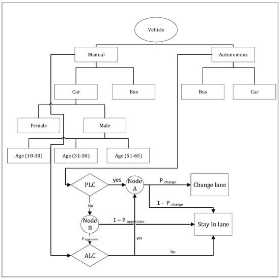
Figure 1.
Flow chart of the model.
We have attempted to explore the impact of autonomous vehicles on traffic flow characteristics and explicitly the influence of autonomous vehicles on traffic flow rates with different types of manual vehicles, which is driven by people of different gender and age. Since the CA model is efficient in capturing complex traffic dynamics, as mentioned earlier, the simulation of different autonomous and manual vehicles in different traffic scenarios is the foundation of this research, as manual and autonomous vehicles will have different traits. In the model, there are different rules which address the specific maneuvers of vehicles. Such rules are described as follows, in the sequence of how the process is modified at each time step:
The position update is defined as:
The deterministic acceleration is defined as:
The deterministic deceleration is defined as:
The minimum safe distance is defined as:
Table 1 shows symbols and abbreviations used in this study.

Table 1.
Symbols and abbreviations.
Where represents the position of the n-th vehicle, represents the current position of the i-th vehicle, represents the speed of the n-th vehicle, is the maximum speed of the vehicle, (t) represents the speed of the n-th vehicle at time instant t, represents the front distance of the vehicle, represents the length of the vehicle, and represent the left and right front distance of the vehicle in the target lane, and represent the left and right back distance of the n-th vehicle in the target lane.
3.1. Lane Change Behavior
The lane change behavior of different drivers that occurs on an urban road is diverse. The lane-changing decision process is modeled as a series of three steps: choosing a lane change, choosing a goal lane, and acknowledging gaps. To capture lane change behavior, we have implemented two types of lane change policies. The first one is the aggressive lane change and the second one is the polite lane change policy for the autonomous and manual vehicle, to simulate real-time traffic maneuvers with different vehicles, which are the basis of this study. We also added a probability factor for the lane-change transition, as in some situations, even if the situation is in their favor, vehicles may not choose to switch lanes. Besides, the front length of vehicles in the target lane should be greater than the minimum safe range (headway) for the lane change. Changing the lane in any direction is appropriate. The first preference is given in the template to switching to the left lane. If the situation is not suitable, however, it is appropriate to change to the right lane rules. If the vehicles are unable to change lane in either direction, they must shift their speed and remain in the same lane. There is another restriction on buses so, that both autonomous buses (ABs) and manual buses (MBs) can travel only on the first and second lanes, and cars can use any lanes to simulate real-world traffic maneuvers. There are different nomenclatures for both the right lane change and the left shift laws.
3.2. Polite Lane Change Policy
MOBIL (Minimizing Overall Braking Induced by changes to the road) is used to tackle the adjustment of the cooperative lane of smart vehicles. MOBIL emulates the lane-changing decision as a trade-off between the motivation of a vehicle planning to change lane, to gain a higher speed, and the courtesy this vehicle will nonetheless show, causing the least possible inconvenience to the adjacent vehicles in the target lane. In polite lane change policy following the MOBIL logic, during lane change, the vehicle will not disturb the speed of the vehicles on the adjacent lane. The following criteria are tested first for any vehicle which will change lanes from the left side. (A) For any n vehicle, by increasing the speed, the vehicle first reaches the minimum safe range. (B) The front range in the target lane shall be verified after hitting the minimum safe distance. (C) Finally, the speed of that n vehicle in the target lane should be higher than that of the rear vehicle in order to change the lane.
Here, represents the vehicle’s maximum speed, and represents the front distance of the vehicle on the driving path. Similar respectful lane change nomenclature refers to the case of the right lane change. If the vehicle does not follow the left-wing shift requirements, the vehicle must test the possibility of changing to the right lane.
There are two additional rules for dealing with the cooperative lane change of two AVs.
3.3. Aggressive Lane Change Policy
The aggressive lane change policy (ALC) represents a collection of lane-changing rules that are more practical than the polite lane change policy (PLC), especially for manual vehicles. Research on manual vehicles’ lane-changing behavior indicates that faster preceding vehicles will allow the following drivers to consider overtaking them in many circumstances [62,63]. Unlike the rules of the polite lane change policy, the vehicle does not have to reach the minimum safe distance by increasing the speed for any n vehicles. We also incorporated the probability factor for violent lane-change movement, as in some situations, even if the situation is in their favor, vehicles may not choose to switch lanes. They can change lanes even though in the driving lane the distance from the previous vehicle is greater than the minimum safe distance. For example, if the front and back gap in the target lane is three cells and the speed is higher than that of the back vehicle in the target lane, the manual vehicle (age: 18–30) will follow the aggressive lane behavior in the target lane. This is similar to what happens with the other vehicles. Therefore, 95% of drivers can only choose to change lanes if the rear spacing on the target lane is greater than the safe distance or if their speed is higher than that of the corresponding vehicles on the target lane [64,65].
Figure 2 represents the lane-changing behavior pattern of a simple case in which a standard manual car is willing to change lane. It will check the conditions of ALC and, if they are met, it will change lane on the basis of an acceptable probability. Figure 3 presents the complete schematic diagram of the proposed model. SF, in Figure 2, stands for minimum front safety distance.
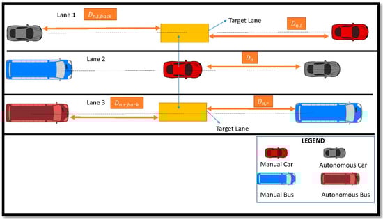
Figure 2.
Lane-changing behavior pattern of a simple case.
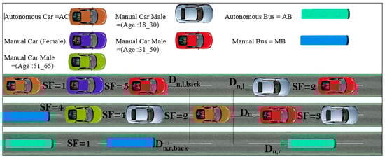
Figure 3.
Schematic diagram of the model.
3.4. Numerical Simulation
The latest CA model was created using MATLAB. Every vehicle is specified by its own class, as mentioned earlier. The class has several attributes, including ID, size, lane travel, distance from back-space, distance from front-space, location, direction, maximum speed, classified according to gender and a further subdivision according to age delay, and type. For simulation tests, as shown in Figure 3, a three-lane freeway stretch without on/off ramps was considered. Each lane is measured by L, and 10,000 m is the total length of the freeway. The size of the cell is 5 m. The size of each car is 1 cell. The bus is twice as long as the car, i.e., the bus covered 2 cells. The maximum speed of the car and the bus is 80 km/h and 60 km/h respectively. Any car’s speed is at one of the five distinct points, 0–4 cells per phase of the time. “0” means that the vehicle is not moving, while “4” means that the vehicle can move through 4 cells in a one-time phase, with a maximum speed of 80 km/h, respectively.
In comparison, every autonomous bus (AB) and manual bus (MB) has a maximum speed of 60 km/h, meaning that it can drive through 3 cells in a second. All autonomous vehicles differ in terms of headway, reaction delay, and lane change maneuvers from their counterparts. We also implanted the possibility of unpredictable braking in all manual vehicles, as the driver is unable to maintain a constant speed.
Due to their lower reaction delay, the minimum safe distance is specified as 1 cell for each autonomous vehicle, while the minimum safe distance for the manual car (age: 18–30), (age: 31–50), and (age: 51–65) is 2, 3, and 4 cells, respectively. On the other hand, the minimum safe distance is 5 cells for the manual vehicle, which is driven by a female. The manual bus has a safe distance of 4 cells. According to AASHTO (American Association of State Highway Officials) [66], the perception reaction time is 2.5 s. Based on this information, we have different sets of the reaction time period, which for the male driver (age: 18–30), (age: 31–50), and (age: 51–65) is 2,3, and 4, respectively, and for the female driver 4 s. Table 2 shows the attributes of different types of vehicles simulated in the model.
Table 2.
Vehicle class.
The minimum distance for the front (previous vehicle) and back (following vehicle) for AC and AB is 2 cells, in furtherance of a shift to the target lane. For the male driver (age: 18–30), the minimum lane change length in the target lane for the front and back is 3 cells. For the male drivers (age: 31–50) and (age: 51–65), the minimum distance for a lane change in the target lane is 4 and 5 cells for the front and back, respectively. For MB, the minimum front and back distance for lane change is 5 cells. For the female, driver according to the reaction time and safe distance, the lane change distance should be more than 5 cells. The vehicles must remain in the same lane if the distance in the target lane is not more than the safe distance. The density (k), average speed and flow rate (q) are determined by the following formula.
Different combinations of vehicles were modeled at varying penetration levels and random brake, PLC, and ALC values. All the scenarios include different penetration rates of autonomous vehicles with the different types of manual vehicles, in order to explicitly highlight their significance in the network. For each case, the simulation was performed with 1000-time steps.
4. Results
Multiple scenarios with different compositions have been simulated for the purposes of the current research. The comparisons made in each scenario are based upon traffic fundamentals diagrams, i.e., speed, density and flow rate. In Scenarios 1 to 3, different compositions of autonomous cars (ACs), manual cars (MCs), ABs, and MBs have been adopted to understand the impact of heterogeneous traffic flow on the overall capacity of the network in the presence of different autonomous vehicles and different manual vehicles. As mentioned before, the manual cars have been further categorized into male and female drivers, and male drivers were further subcategorized based on age groups. In all of these scenarios, the value of PLC and ALC was kept constant at 0.5 to highlight the influence of different gender and age group cars on the overall transportation system in the presence of autonomous vehicles, and to determine whether autonomous vehicles can positively change the network’s capacity. In Scenario 4, the percentage of vehicles was kept constant, with variable values of ALC and PLC. The objective of Scenario 5 is to understand the paramount importance of different lane-changing behaviors in mixed traffic flows. It was emphasized here that in the adopted model the autonomous vehicles can follow both PLC and ALC behaviors, whereas manual vehicles will only follow ALC, irrespective of gender and age. Table 3 lists the detailed compositions of all simulated scenarios in this study.
Table 3.
Scenarios based on different compositions.
4.1. Scenario 1
Figure 4 presents the speed–density relationship of Scenario 1. Figure 5 documents the speed–flow rate relationship of Scenario 1, and Figure 6 denotes the flow rate–density relationship. There are five types of simulation in this scenario. The goal of this arrangement is to assess the performance of the model in which AC runs parallel with MC (different genders and age groups).
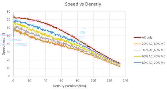
Figure 4.
Speed–Density curve of Scenario 1.
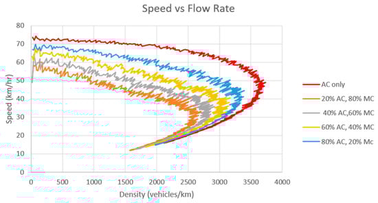
Figure 5.
Speed–Flow Rate curve of Scenario 1.
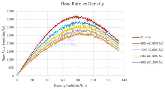
Figure 6.
Flow Rate–Density curve of Scenario 1.
In this setup, the composition is the following: 100% AC, 20% AC + 80% MC, 40% AC + 60% MC, 60% AC + 40% MC, 20% AC + 80% MC with ALC = 0.5 and PLC = 0.5.
4.2. Scenario 2
Figure 7 presents the speed–density relationship of Scenario 2. Figure 8 documents the speed–flow rate relationship of Scenario 2, and Figure 9 denotes the flow rate–density relationship.
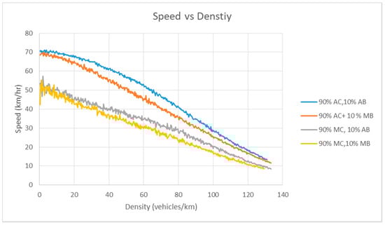
Figure 7.
Speed–Density curve of Scenario 2.
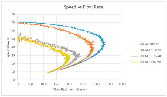
Figure 8.
Speed–Flow Rate curve of Scenario 2.
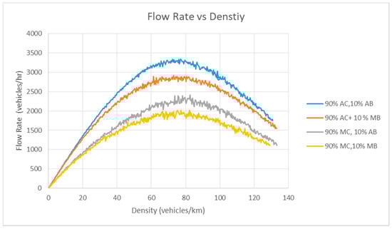
Figure 9.
Flow Rate–Density curve of Scenario 2.
In this setup, the composition is the following: 90% AC + 10% AB, 90% AC + 10% MB, 90% MC + 10% AB, 90% MC + 10% MB with ALC = 0.5 and PLC = 0.5.
The goal of this simulation is to study the impact of buses, including AB and MB, in a heterogeneous traffic flow alongside AC and MC. In real-time traffic, buses also have a significant capacity on the road due to their large size and difficulties in maneuverability.
4.3. Scenario 3
Figure 10 presents the speed–density relationship in Scenario 3. Figure 11 documents the speed–flow rate relationship of Scenario 3, and Figure 12 denotes the flow rate–density relationship.
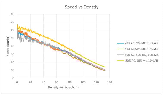
Figure 10.
Speed–Density curve of Scenario 3.
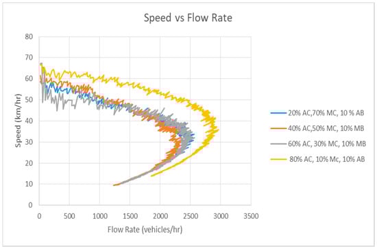
Figure 11.
Speed–Flow Rate curve of Scenario 3.
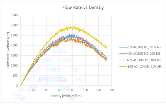
Figure 12.
Flow Rate–Density curve of Scenario 3.
In this setup, the composition is the following: 20% AC + 70% MC + 10% AB, 40% AC + 50% MC + 10% MB, 60% AC + 30% MC + 10% MB, 80% AC + 10% MC + 10% AB with ALC = 0.5 and PLC = 0.5.
The objective of this simulation is to study the impact of buses, including AB and MB, in the presence of MC. In the near future, AC and AB will have to run concurrently with MC in different proportions.
4.4. Scenario 4
Figure 13 presents the speed–density relationship of Scenario 4. Figure 14 documents the speed–flow rate relationship of scenario 4, and Figure 15 denotes the flow rate–density relationship.
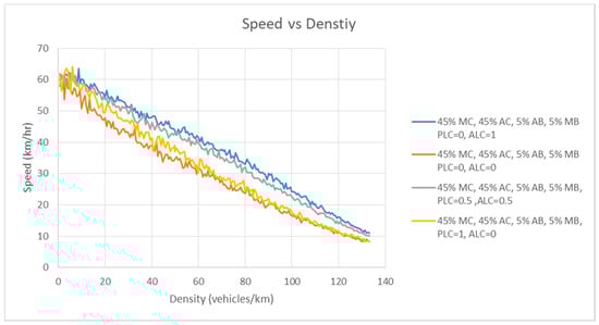
Figure 13.
Speed–Density curve of Scenario 4.
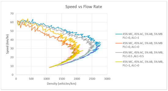
Figure 14.
Speed–Flow Rate curve of Scenario 4.
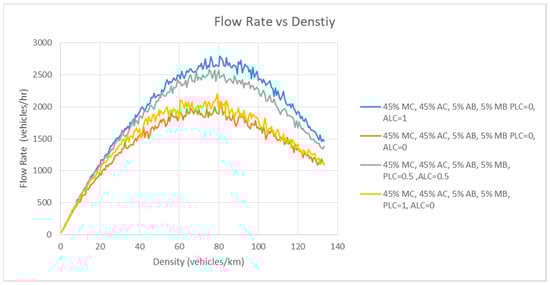
Figure 15.
Flow Rate–Density curve of Scenario 4.
In this setup, the composition is the following: 45% MC + 45% AC + 5% AB + 5% MB with different values of ALC = 0,0.5 and 0.1, and PLC = 0, 0.5 and 0.1.
There are four different types of simulation in this setup. The goal of this simulation is to study the impact of the varying level of lane-changing behavior in the model.
5. Discussions
The major conclusions of each scenario are described in Table 4:
Table 4.
Major Conclusion.
As per the results and discussions of this study, it is imperative to consider the potential strategies before the deployment of autonomous vehicles at a large scale, as merely including them randomly is not a guarantee that the traffic flow rate will improve considerably. The modeling of junctions and merging of access points under heterogeneous conditions, including autonomous vehicles and different drivers, can also provide an insight into the best optimal scenario to get the most out of automation technology. Currently, this study assumes a deterministic influx of vehicles. Stochastic modeling of different heterogeneous scenarios can be modeled to assess the performance of autonomous vehicles and their potential impact on the traffic flow rate.
6. Conclusions
In this paper, we have investigated the heterogeneity in traffic by comparing different modes of autonomous vehicles (autonomous cars and autonomous buses) and manual vehicles (manual cars and manual buses). Manual cars were then further divided into two categories, based on gender. The male drivers were further subdivided based on different age groups, i.e., young, adult, and old. A new cellular automata model was developed to include the unique characteristics and attributes of different drivers and vehicles by simulating real-time traffic scenarios. Moreover, two different lane-changing behavior methodologies were adopted, i.e., aggressive lane-changing behavior and polite lane-changing behavior. In each scenario, different arrangements were set up to study the concept of heterogeneity in different conditions. Another assumption incorporated in the model was that manual vehicles would follow only aggressive lane-changing behavior and autonomous vehicles can follow both polite and aggressive lane-changing behavior.
The main findings of this study can be summarized as follows:
Currently, in real-time traffic, heterogeneous traffic is further divided based on genders and age groups. All of these groups have different characteristics, response time, and actions, depending upon their cognitive functionalities. This drawback can be eliminated by incorporating autonomous vehicles in the daily traffic volume. With the help of this newly developed cellular automata model, the impact of autonomous vehicles in these mixed traffic flows is highlighted. With the increase of the penetration rate of autonomous vehicles, the traffic flow rate can be increased considerably, irrespective of age or gender differences. The mere inclusion of only 20% of autonomous vehicles can increase the overall traffic flow rate.
When both manual vehicles and autonomous vehicles are allowed to change lanes aggressively, the capacity of the network increases substantially. In contrast, when autonomous vehicles follow a polite lane-changing behavior, the flow rate is similar to the case when none of the vehicles are allowed to change lanes. Thus, polite lane change has a negligible impact on the flow rate.
Autonomous vehicles have the potential to increase the capacity of roads, as reported in previous studies, but none of the studies have tried to include the concept of heterogeneity based on gender and age groups in their traffic flow models. This novel study has attempted to cover this drawback by simulating different scenarios. This work can be further extended by studying the impact of heterogenous traffic and autonomous vehicles on a city-wide level, through traffic assignments, and on signalized and unsignalized junctions.
Author Contributions
M.T. and F.A.K. proposed the methodology, prepared wrote the model; H.N., H.Y., X.Q. wrote the Introduction and Literature Review; M.T. and F.A.K. performed the simulations, analyzed and wrote the results and conclusions; S.M.A.R., T.W. and H.L. provided valuable opinions during the manuscript writing. All authors have read and agreed to the published version of the manuscript.
Funding
This research was funded by the “Research on Transportation Strategy for a Powerful Nation” (2017ZD07), the major consulting project of the Chinese Academy of Engineering (No. 2017ZD07).
Conflicts of Interest
The authors declare no conflict of interest.
References
- Office of Highway Policy Information. Public Data for Highway Statistics; Office of Highway Policy Information: Washington, DC, USA, 2017.
- Center for Disease Control. Injury Prevention and Control: Data and Statistics; Center for Disease Control: Atlanta, GA, USA, 2011.
- Hayes, B. Leaving the driving to it. Am. Sci. 2011, 99, 362–366. [Google Scholar] [CrossRef]
- World Health Organization. Global Status Report on Road Safety. 2018. Available online: https://www.who.int/violence_injury_prevention/road_safety_status/2018/en/ (accessed on 17 June 2018).
- Chen, H.Y.; Ivers, R.; Martiniuk, A.; Boufous, S.; Senserrick, T.; Woodward, M.; Stevenson, M.; Norton, R. Socioeconomic status and risk of car crash injury, independent of place of residence and driving exposure: Results from the DRIVE Study. J. Epidemiol. Community Health 2010, 64, 998–1003. [Google Scholar] [CrossRef] [PubMed]
- Chen, L.-H. Teenager Driver Crash Risk: The Effect of Passengers; Johns Hopkins University: Baltimore, MD, USA, 1999. [Google Scholar]
- Preusser, D.F.; Ferguson, S.A.; Williams, A.F. The effect of teenage passengers on the fatal crash risk of teenage drivers. Accid. Anal. Prev. 1998, 30, 217–222. [Google Scholar] [CrossRef]
- Elvik, R. Why some road safety problems are more difficult to solve than others. Accid. Anal. Prev. 2010, 42, 1089–1096. [Google Scholar] [CrossRef] [PubMed]
- McCartt, A.T.; Shabanova, V.I.; Leaf, W.A. Driving experience, crashes and traffic citations of teenage beginning drivers. Accid. Anal. Prev. 2003, 35, 311–320. [Google Scholar] [CrossRef]
- Vachal, K.; Faculty, R.; Malchose, D. What can we learn about North Dakota’s youngest drivers from their crashes? Accid. Anal. Prev. 2009, 41, 617–623. [Google Scholar] [CrossRef]
- Walsh, S.P.; White, K.M.; Hyde, M.; Watson, B. Dialling and driving: Factors influencing intentions to use a mobile phone while driving. Accid. Anal. Prev. 2008, 40, 1893–1900. [Google Scholar] [CrossRef]
- Harbeck, E.; Glendon, I. How reinforcement sensitivity and perceived risk influence young drivers’ reported engagement in risky driving behaviors. Accid. Anal. Prev. 2013, 54, 73–80. [Google Scholar] [CrossRef]
- Hancock, P. Are Autonomous Cars Really Safer than Human Drivers? Available online: https://www.scientificamerican.com/article/are-autonomous-cars-really-safer-than-human-drivers/ (accessed on 3 February 2018).
- University of Idaho. Traffic Flow Theory, Types of Traffic Flows. August 2003. Available online: http://www.webpages.uidaho.edu/niatt_labmanual/chapters/trafficflowtheory/theoryandconcepts/TypesOfTrafficFlow.htm (accessed on 6 April 2020).
- AbuAli, N.; Abou-Zeid, H. Driver behavior modeling: Developments and future directions. Int. J. Veh. Technol. 2016, 2016, 6952791. [Google Scholar] [CrossRef]
- Mamidi Kiran Kumar, V.K.P. Driver behavior analysis and prediction models. Int. J. Comput. Sci. Inf. Technol. 2015, 6, 3328–3333. [Google Scholar]
- Kumagai, T.; Sakaguchi, Y.; Okuwa, M.; Akamatsu, M. Prediction of driving behavior through probabilistic inference. In Proceedings of the 8th International Conference Engineering Applications of Neural Networks, Malaga, Spain, 8–10 September 2003. [Google Scholar]
- Gazis, D.C.; Herman, R.; Rothery, R.W. Nonlinear follow-the-leader models of traffic flow. Oper. Res. 1961, 9, 545–567. [Google Scholar] [CrossRef]
- Jin, S.; Wang, D.; Huang, Z.-Y.; Tao, P. Visual angle model for car-following theory. Phys. A Stat. Mech. Appl. 2011, 390, 1931–1940. [Google Scholar] [CrossRef]
- Jin, S.; Wang, D.-H.; Yang, X.-R. Non-lane-based car-following model with visual angle information. Transp. Res. Rec. 2011, 2249, 7–14. [Google Scholar] [CrossRef]
- Jin, S.; Wang, D.; Xu, C.; Huang, Z.-Y. Staggered car-following induced by lateral separation effects in traffic flow. Phys. Lett. A 2012, 376, 153–157. [Google Scholar] [CrossRef]
- Berling-Wolff, S.; Wu, J. Modeling urban landscape dynamics: A review. Ecol. Res. 2004, 19, 119–129. [Google Scholar] [CrossRef]
- Sven Maerivoet, B.D.M. Cellular automata models of road traffic. Phys. Rep. 2005, 419, 1–64. [Google Scholar] [CrossRef]
- Barlovic, R.J.E.; Froese, K.; Knospe, W.; Neubat, L.; Schreckenberg, M.; Wahle, J. Online Traffic Simulation with Cellular Automata. In Traffic and Mobility: Simulation-Economics-Environment, Institut für Kraftfahrwesen; RWTH Aachen: Duisburg, Germany, 1999; pp. 117–134. [Google Scholar]
- Chowdhury, D.A. Schadschneider, Statistical physics of vehicular traffic and some related systems. Phys. Rep. 2000, 329, 199–329. [Google Scholar] [CrossRef]
- Mu, R.; Yamamoto, T. An Analysis on Mixed Traffic Flow of Conventional Passenger Cars and Microcars Using a Cellular Automata Model. In Proceedings of the 8th International Conference on Traffic and Transportation Studies, Changsha, China, 1–3 August 2012. [Google Scholar]
- Wu, W.; Liu, Y.; Xu, Y.; Wei, Q.; Zhang, Y. Traffic Control models based on cellular automata for at-grade intersections in autonomous vehicle environment. J. Sens. 2017, 2017, 9436054. [Google Scholar] [CrossRef]
- Qu, X.; Yang, M.; Yang, F.; Ran, B.; Li, L. An Improved Single-Lane Cellular Automaton Model considering Driver’s Radical Feature. J. Adv. Transp. 2018, 2018, 3791820. [Google Scholar] [CrossRef]
- Gao, Y.; Zhou, Q.; Chai, C.; Wong, Y.D. Safety impact of right-turn waiting area at signalized junctions conditioned on driver’s decision-making based on fuzzy cellular automata. Accid. Anal. Prev. 2019, 123, 341–349. [Google Scholar] [CrossRef]
- Evans, L. Traffic Safety and the Driver; Science Serving Society; Van Nostrand Reinhold: New York, NY, USA, 1991. [Google Scholar]
- McKenna, F.P.; Waylen, A.; Burkes, M. Male and Female Drivers: How Different are They? TRB: Washington, DC, USA, 1998. [Google Scholar]
- Waylen, A.; McKenna, F. Cradle Attitudes-Grave Consequences-The Development of Gender Differences in Risky Attitudes and Behaviour in Road Use; TRB: Washington, DC, USA, 2002. [Google Scholar]
- Parker, D.; West, R.; Stradling, S.; Manstead, A. Behavioural characteristics and involvement in different types of traffic accident. Accid. Anal. Prev. 1995, 27, 571–581. [Google Scholar] [CrossRef]
- Lancaster, R.; Ward, R. The Contribution of Individual Factors to Driving Behaviour: Implications for Managing Workrelated Road Safety; Report No. 20; Health and Safety Executive: London, UK, 2002. [Google Scholar]
- Chipman, M.L.; MacGregor, C.G.; Smiley, A.M.; Lee-Gosselin, M. Time vs. distance as measures of exposure in driving surveys. Accid. Anal. Prev. 1992, 24, 679–684. [Google Scholar] [CrossRef]
- Waller, P.F.; Elliott, M.R.; Shope, J.T.; Raghunathan, T.E.; Little, R.J. Changes in young adult offense and crash patterns over time. Accid. Anal. Prev. 2001, 33, 117–128. [Google Scholar] [CrossRef]
- Norris, F.H.; Matthews, B.; Riad, J.K. Characterological, situational, and behavioral risk factors for motor vehicle accidents: A prospective examination. Accid. Anal. Prev. 2000, 32, 505–515. [Google Scholar] [CrossRef]
- Mizell, L.; Joint, M.; Connell, D. Aggressive Driving: Three Studies; TRB: Washington, DC, USA, 1997. [Google Scholar]
- Loughran, D.; Seabury, S.; Zakaras, L. What Risks Do Older Drivers Pose to Traffic Safety? RAND Corporation: Santa Monica, CA, USA, 2007. [Google Scholar]
- Federal Highway Administration. National Household Travel Survey; Federal Highway Administration: Washington, DC, USA, 2001.
- Tefft, B.C. Risks older drivers pose to themselves and to other road users. J. Saf. Res. 2008, 39, 577–582. [Google Scholar] [CrossRef]
- Staplin, L.; Lococo, K.H.; Martell, C.; Stutts, J. Taxonomy of Older Driver Behaviors and Crash Risk; National Highway Traffic Safety Administration: Washington, DC, USA, 2012.
- Fisk, D.; Charness, N.; Czaja, S.J.; Rogers, W.A.; Sharit, J. Designing for Older Adults: Principles and Creative Human Factors Approaches, 2nd ed.; CRC Press: Boca Raton, FL, USA, 2009. [Google Scholar]
- Ivers, R.; Senserrick, T.; Boufous, S.; Stevenson, M.; Chen, H.Y.; Woodward, M.; Norton, R. Novice drivers’ risky driving behavior, risk perception, and crash risk: findings from the DRIVE study. Am. J. Public Health 2009, 99, 1638–1644. [Google Scholar] [CrossRef]
- Ali, E.K.; El-Badawy, S.; Shawaly, E.A. Young drivers behaviour and its influence on traffic accidents. J. Traff. Logist. Eng. 2014, 2, 45–51. [Google Scholar] [CrossRef]
- Duke-Elder, S. Francisus cornelis donders. Br. J. Ophthalmol. 1959, 8, 43–65. [Google Scholar]
- Halpern, D.F. Sex Differences in Cognitive Abilities; Erlbaum: Hillsdale, NJ, USA, 1992. [Google Scholar]
- Herlitz, A.; Love´n, J. Sex differences in cognitive functions. Acta Psychol. Sin. 2009, 41, 1081–1090. [Google Scholar]
- Reed, T.; Vernon, P.A.; Johnson, A.M. Sex difference in brain nerve conduction velocity in normal humans. Neuropsychologia 2004, 42, 1709–1714. [Google Scholar] [CrossRef]
- Lahtela, K.; Niemi, P.; Kuusela, V. Adult visual choice-reaction time, age, sex and preparedness: A test of Welford’s problem in a large population sample. Scand. J. Psychol. 1985, 26, 357–362. [Google Scholar] [CrossRef] [PubMed]
- Bunce, D.; Tzur, M.; Ramchurn, A.; Gain, F.; Bond, F.W. Mental health and cognitive function in adults aged 18 to 92 years. J. Geronto. Ser. B Psychol. Sci. 2008, 63, 67–74. [Google Scholar] [CrossRef] [PubMed]
- Fairweather, H.; Hutt, S.J. Sex differences in a perceptual-motor skill in children. In Gender Differences: Their Ontogeny and Significance; Churchill Livingstone: Edinburgh, UK, 1972; pp. 159–175. [Google Scholar]
- Deary, I.J.; Der, G. Reaction time, age and cognitive ability: Longitudinal findings from age 16 to 63 years in representative population samples. Aging Neurosci. Cogn. 2005, 12, 187–215. [Google Scholar] [CrossRef]
- Dykiert, D.; Der, G.; Starr, J.M.; Deary, I.J. Sex Differences in reaction time mean and intraindividual variability across the life Span. Dev. Psychol. 2012, 48, 1262–1276. [Google Scholar] [CrossRef]
- Gazis, D.C.; Herman, R.; Rothery, R.W. Non-linear follow the leader models of traffic flow. Oper. Res. 1961, 9, 545–567. [Google Scholar] [CrossRef]
- Newell, G.F. Non-linear effects in the dynamics of car following. Oper. Res. 1961, 9, 209–229. [Google Scholar] [CrossRef]
- Van Winsum, W.; De Waard, D.; Brookhuis, K. Lane change manoeuvres and safety margins. Transp. Res. Transp. Res. 1999, 2, 139–149. [Google Scholar] [CrossRef]
- Zheng, Z.; Ahn, S.; Monsere, C.M. Impact of traffic oscillations on freeway crash occurrences. Accid. Anal. Prev. 2010, 42, 626–636. [Google Scholar] [CrossRef]
- Sen, B.; Smith, J.D.; Najm, W.G. Analysis of Lane Change Crashes; John, A., Ed.; Volpe National Transportation Systems Center: Cambridge, MA, USA, 2003.
- Gipps, P.G. A model for the stucture of lane chaning models. Transp. Res. B 1986, 20, 403–414. [Google Scholar] [CrossRef]
- Hidas, P. Modelling lane changing and merging in microscopic traffic simulation. Transp. Res. Part C 2002, 10, 351–371. [Google Scholar] [CrossRef]
- George Oketch, T. New modeling approach for mixed-traffic streams with nonmotorized vehicles. Transp. Res. Rec. 2000, 1705, 61–69. [Google Scholar] [CrossRef]
- Lee, S.E.; Olsen, E.C.; Wierwille, W.W. A Comprehensive Examination of Naturalistic Lane-Changes; National Highway Traffic Safety Administration: Washington, DC, USA, 2004.
- Kim, S.-W.; Liu, W. Cooperative autonomous driving: A mirror neuron inspired intention awareness and cooperative perception approach. IEEE Intell. Transp. Syst. Mag. 2016, 8, 23–32. [Google Scholar] [CrossRef]
- Fei, L.; Zhu, H.; Han, X. Analysis of traffic congestion induced by the work zone. Phys. A Stat. Mech. Appl. 2016, 450, 497–505. [Google Scholar] [CrossRef]
- Highway, A.A.O.S.; Officials, T. A Policy on Geometric Design of Highways and Streets; American Association of State Highway Offical Transportation: Washington, DC, USA, 2011. [Google Scholar]
© 2020 by the authors. Licensee MDPI, Basel, Switzerland. This article is an open access article distributed under the terms and conditions of the Creative Commons Attribution (CC BY) license (http://creativecommons.org/licenses/by/4.0/).