1. Introduction
In the early 1970s, with the link between gold and US dollars being severed and the collapse of the pegged exchange rate regime, a new monetary system, the floating exchange rate regime, arose. Nevertheless, exchange rates were not entirely determined by the market during the transitional period, while regular foreign exchange interventions (FXIs) occurred in a number of countries. FXIs are generally motivated by several factors, one of which is coordination with corresponding trade policies. South Korea is a typical export-oriented economy that relies heavily on exports to drive its economic growth. However, every coin has two sides. A relatively weaker Korean won contributes positively to exports and a current account surplus but may also lead to a wide spectrum of retaliatory actions, such as non-tariff barriers or anti-dumping duties, launched by the importing partner. As such, the Bank of Korea (BOK) makes interventions to adjust the exchange rate to targeted levels as needed.
On 2 July 1997, Thailand declared implementation of the floating exchange rate system instead of the fixed one, which incurred a financial crisis throughout Southeast Asia, including Thailand, Indonesia, South Korea and so forth. The Asian foreign exchange crisis not only put a damper on many Southeast Asian economies but also depleted a significant portion of their foreign reserves. In particular, South Korean’s incapability of defending against external shocks was thoroughly exposed amid crisis as it is a chaebol-dominated economic structure with excessive foreign borrowings. Worse still, the Korean won’s exchange rate has long been deviated from long-term equilibrium under a managed floating exchange rate system. Namely, maintaining overvaluation of the Korean won accelerated the collapse of the economy. Against that backdrop, the South Korean government was compelled to liberalize the financial market and capital flows in return for receiving IMF loans and foreign aid. Since then, the government has been plagued by a dilemma of how to address the growing disparity between domestic assets and foreign assets and between medium-/long-term and short-term capital while maintaining a highly open capital market. Given that the aforementioned imbalances would inevitably elicit vulnerability and high volatility in the domestic currency, the monetary authority is supposed to steer intervention appropriately. The aim is to strengthen the won’s ability to shield the economy from external shocks. On the flip side, capricious fluctuations in the market can be mapped into the defensive behaviors of market participants. For instance, manufacturers are inclined to pass on “fear of future uncertainties” to consumers through price hikes, which then signal inflationary pressure. For this reason, there is a broad consensus that the exchange rate can serve as a barometer for inflation.
Not until the crisis broke out in 1997 did the South Korean government quit espousing a ‘high debts, low reserves’ tenet. In the meantime, the foreign exchange reserves were about to be dried up. The economic malaise raised awareness of the importance of accumulating reserves. Thereafter, in an effort to ameliorate the liquidity of balance of payment (BOP), the South Korean government, over an extended period, accelerated the opening-up of capital (financial) accounts and loosened restrictions on foreign capital inflows. The accumulation of foreign exchange reserves, on the one hand, is known as an effective buffer and, on the other hand, has been criticized for its holding costs (e.g., opportunity costs and costs of sterilization) and potential risks (e.g., inflation and depreciation of dollarized assets). Therefore, the intermediate target has recently shifted towards dollar liquidity. All participants and transactions are under few restraints in a market with high liquidity. Central banks can become involved in intervention whenever a unilateral aberrant trend in the exchange rate emerges. For instance, the Korean monetary authority attempted to secure high dollar liquidity through swap market during the 2008 global financial crisis. In addition to direct intervention channels such as spot market, forward market as well as swap market, indirect intervention tools—anticipatory guidance—were also employed to prevent speculation.
It is believed that the higher the elasticity of capital flows relative to interest rate changes is under a floating exchange rate system, the more obvious the effect of the non-sterilized intervention. In the wake of a sharp increase in money supply, overall price levels will eventually be driven up. Hence, the BOK has been implementing sterilized intervention in a bid to guarantee the effectiveness of the independent monetary policy. In other words, the BOK should adjust the won’s exchange rate based on the premise that interest rate remains unchanged, and the real interest rates as a basic measure to intervene in forex have been low, leaving little room to utilize. Moreover, the BOK resorts to choking off excessive demand for money by issuing Monetary Stabilization Bonds (MSBs) through its open market operations (OMO). Paradoxically, raising bond yields (lowering bond prices) gives rise to higher market interest rates followed by net capital inflows due to interest rate spreads. This then stimulates the BOK to go on to the next sterilized intervention. In practice, the efficacy of sterilized intervention remains disputed both empirically and theoretically, which is one of the motivations of our study. In addition, it is undeniable that the magnitude of intervention and the degree of substitutability between domestic and foreign financial assets play a vital role.
Simply put, the central banks meddle in forex with the following multifaceted considerations: (i) In the financial sector, stabilizing the market portends that the macroeconomy performance is, to a large degree, immune to risks potentially aroused by the fluctuation of the capital (financial) account. (ii) Regarding the substantial economy, particularly in emerging market economies (EMEs), moderate depreciation of the domestic currency facilitates product competitiveness, further improving exports and their current accounts. (iii) Given the interaction mechanism between the exchange rate and the interest rate, monetary authorities are likely to embark on intervention amid rising concerns over inflation.
In this study, we design a threshold vector autoregression (TVAR) model to estimate the impact of intervention in Korean forex on multiple macroeconomic indicators under various regimes and shocks. Most relevant studies fail to give sufficient consideration to specifying the heterogeneity of foreign reserve shocks. Therefore, we cast doubt on whether the responses of the current account, capital (financial) account, exchange rate volatility, short-term interest rate and long-term interest rate are homogenous under different histories, directions or magnitudes of external shocks. The outstanding contribution of this paper is to investigate the impulse responses related to external foreign reserve shocks. We do this by unfolding each of the related endogenous variables. In diverse circumstances, these variables vary to a greater or lesser degree from their corresponding functions. These findings have yet to be extrapolated to other small open economies in future studies.
The remainder of this paper is organized as follows:
Section 2 provides a literature review,
Section 3 presents the data and model specification, and
Section 4 unveils the empirical results, followed by concluding remarks in
Section 5.
2. Literature Review
The price of a country’s currency, seen as a commodity, is essentially determined by the relationship between supply and demand in the forex market. The fluctuations of the exchange rate exercise great influence on macroeconomic operation [
1] and the implementation of monetary policy [
2,
3]. From the micro perspective, both enterprises and individuals are more likely to succumb to the risks under a floating exchange rate regime than under a fixed regime since production and consumption behaviors tend to change accordingly when dealing with uncertainty [
4]. Under a dirty float (managed float regime) the central bank, one of the key participants, will occasionally be obliged to intervene in the forex market. This occurs when there are deviations from target zones or when there is drastic short-term volatility. However, there has long been controversy over many aspects of such interventions, including motivation, channels [
5], efficacy [
6], costs and the impacts on an array of macroeconomic indices.
First, what are the driving factors that cause central banks to engage in FXI? [
7] clarify that numerous EMEs took financial stability as their first priority after the financial crisis because their capital flows were subject to untenable volatility. [
8] comprehensively uncovers that there are two reasons motivating the BOK to intervene: first, to dampen excessive exchange rate volatility and, second, to address the shortage of foreign reserves (especially during a crisis) and keep dollar liquidity.
Subsequently, regarding the channels and efficacy of interventions, [
9] illustrate that the signaling channel through which the People’s Bank of China (PBOC) carries out intervention is weak and not as effective as an actual intervention. A plausible reason is that official statements are often seen as a neutral stance in the intervention. [
10] gives a detailed theoretical derivation to confirm that verbal intervention in EMEs is futile if the central banks frequently make an attempt to ‘cry wolf’ (see also [
11]).In contrast, [
12] reveals that the verbal interventions released by the Swiss National Bank (SNB) are capable of curbing the future volatility of the franc against the euro, thus achieving the desired level due to the credibility of the SNB. With respect to the portfolio balance channel, when endogeneity is taken into account, [
13] demonstrates that a massive intervention for many EMEs is believed to be effective in neutralizing appreciation pressures on domestic currency derived from capital inflows. [
14] employs the tick data of several Latin American countries to draw the conclusion that the first intervention within a day is conducive to mitigating initial exchange rate fluctuations to a lesser extent than subsequent fluctuations (see also [
15]). To cope with the aftermath of the global financial crisis, [
16] investigates several dominant economies in Southeast and East Asia. They disclose that ‘leaning-against-the-wind’ intervention is an advisable countermeasure over the short haul but not a panacea. A long-term strategy is to establish joint intervention mechanisms externally and put into practice macroprudential policy internally. [
17] empirically sheds light on the influence of market uncertainty, which is a necessary prerequisite for looking into the efficacy of intervention. Their findings point to market uncertainty having an inverse proportional relationship to the effectiveness of intervention. This is because other participants aside from central banks, i.e., speculators and arbitragers, have little influence on the trends in uncertain markets.
Nonetheless, it is of particular note that central banks differ considerably in their responses to diversified shocks, which is referred to as asymmetric policy preference. [
18] captures this phenomenon by studying some EMEs in Asia. They show evidence that the central banks took an aggressive stance against upward pressures in sharp contrast with their sluggish attitude towards depreciation. Similarly, [
19] point out that PBOC acted regularly in the forex after the financial crisis to carry out asymmetric interventions in Chinese yuan owing to a ‘fear of appreciation’. On the other hand, identical intervention seems to trigger asymmetric consequences. [
20] discusses the impact of FXI on interbank exchange rates in Peru and documents that intervention is a relatively effective instrument to lower rather than boost exchange rates. [
21] advocates that asymmetric effects accompany interventions in advanced economies, such as Japan and the USA. Its empirical results reflect that, in the case of misalignment between the Japanese yen and US dollar, intervention results in greater volatility if the exchange rate returns are susceptible to adverse shocks rather than to favorable innovation. In a case study of India, [
22] provides solid evidence that the effects of the Reserve Bank of India (RBI)’s intervention are asymmetric—more effective if exchange rate is lying beyond either the upper or lower bound—by employing a nonlinear model (three-regime threshold VAR model).
Recently, an increasing number of researchers have paid close attention to the costs and other relevant issues since actual interventions entail expenses regardless of their motivation or effectiveness. [
23] shows that both the marginal and total ex-ante average costs of intervention for EMEs are approximately 1.8 times the average costs for advanced economies in each quartile. Additionally, there is a contrast in median marginal cost between light interveners and heavy interveners in terms of ex-post costs, accounting for 10.13% and 3.44% of GDP, respectively. However, the total expenses show no significant difference. [
24] conduct empirical analysis with an extensive panel dataset, suggesting that intervention is lucrative for advanced economies, while EMEs have to take into consideration affordability before intervention.
Last, considering the influence of FXI on the macroeconomy, [
25,
26] show that current account imbalances largely emanate from the accumulation of foreign exchange reserves and foreign assets in EMEs. Specifically, each dollar of intervention yields as much as an equivalent increase in the current account balance, and this far outweighs previous estimations. By designing a GARCH (1,1) model, [
27] outlines that the intervention performed by the RBI effectively attenuates the volatility in the Indian forex. Moreover, [
28] stresses that the exchange rate volatility of domestic currency in Peru is alleviated after a substantial dollar-based intervention, which is in accordance with previous studies. A meta-analysis corroborates that the central banks in EMEs are overwhelmingly superior to those in advanced economies in terms of resources that increase the tendency toward intervention. Therefore, they are more liable to achieve predetermined goals, for instance, keeping the volatility and exchange rates within a reasonable range [
29].
3. Data and Model Specification
In this section, we will analyze the responses of Korea’s current account, capital (financial) account and interest rate to shocks in foreign reserves by employing the following threshold VAR (TVAR) model:
where y
t-d is the threshold variable at delay lag d. I(·) is an indicator function that takes the value of 1 if the threshold variable y
t-d is greater than the threshold γ and 0 otherwise. A
1 and A
2 are the lag polynomial matrices, while ε
t are the structural disturbances. The model can be rewritten as follows:
Y
t denotes the vector of endogenous variables and consists of 5 endogenous variables, which are foreign reserves
reservet, current account
cat, capital (financial) account
kat, exchange rate volatility
fxt and interest rate
irt. We look into the effects of the changes in Korea’s foreign reserves on the changes in short-term interest rate
shortratet and long-term interest rate
longratet, which are the 1-day call rate and the 3-year government bond interest rate in this paper. The data sample is a monthly data sample from 2001M1 to 2017M5.
When estimating the TVAR model, we first need to ensure that all of the data series used are stationary. Thus, we employed the augmented Dicker–Fuller test for the unit root test, and the results are presented in
Table 1. The descriptive statistics of all variables used in this paper are shown in
Table 2. We then use the reserves, current account, capital (financial) account and exchange rate volatility variables and the first-difference form of interest rate in our TVAR model. The endogenous variables of each model can be written as follows:
4. Empirical Results
4.1. Estimation Results
In both Models 1 and 2, we set the exchange rate volatility as the threshold variable and analyze the differences in the responses to the other variables in the model for foreign reserve shocks in different regimes.
Table 3 presents the estimated threshold values of the models proposed in this study. When using exchange rate volatility as the threshold variable, the threshold values are estimated to be 0.9606% and 0.7694% for Model 1 and Model 2, respectively. These results indicate two regimes: the regime of high exchange rate volatility, which includes exchange rate volatility values above 0.9606% (or 0.7694% in the case of Model 2), and the regime of low exchange rate volatility, which includes values lower than 0.9606% (or 0.7694%).
Table 4,
Table 5 and
Table 6 report the estimation results Model 1 for current account, capital account and short-term interest rate, respectively. We have also reported both linear and threshold VAR Model estimation results. For Model 1, we can observe that in all cases, the coefficients of the lagged reserves do not have significant effect on the above-said macroeconomic variable.
Similarly, we have also displayed the estimation results of Model 2 for both linear and threshold VAR Models in
Table 7,
Table 8 and
Table 9. In this case, we have seen that the lagged variable of reserves has significantly positive effect on capital account in the high regime of exchange rate volatility. Yet beyond that, the coefficients of lagged reserves in other cases have been reported insignificant.
4.2. Generalized Impulse Responses
The possibility of endogenous regime-switching in the nonlinear VAR model makes the computation of the impulse response function more complicated in this model than in the linear VAR model. The endogenous regime-switching mentioned here refers to the case in which the shocks initially affect the system in one regime and then switch to another regime. Therefore, we address this problem by computing the generalized impulse response function (GIRF) proposed by [
30]. The GIRF allows us to consider the history of the shock (the regime that the system is initially in), the direction of the shock (whether it is a positive or negative shock) and the magnitude of the shock (whether it is a small shock, which is set to be 1 SD, or a large shock, which is set to be 2 SD). In addition, GIRFs are not affected by the ordering of endogenous variables; thus, the ordering of the variables in the system is no longer a concern.
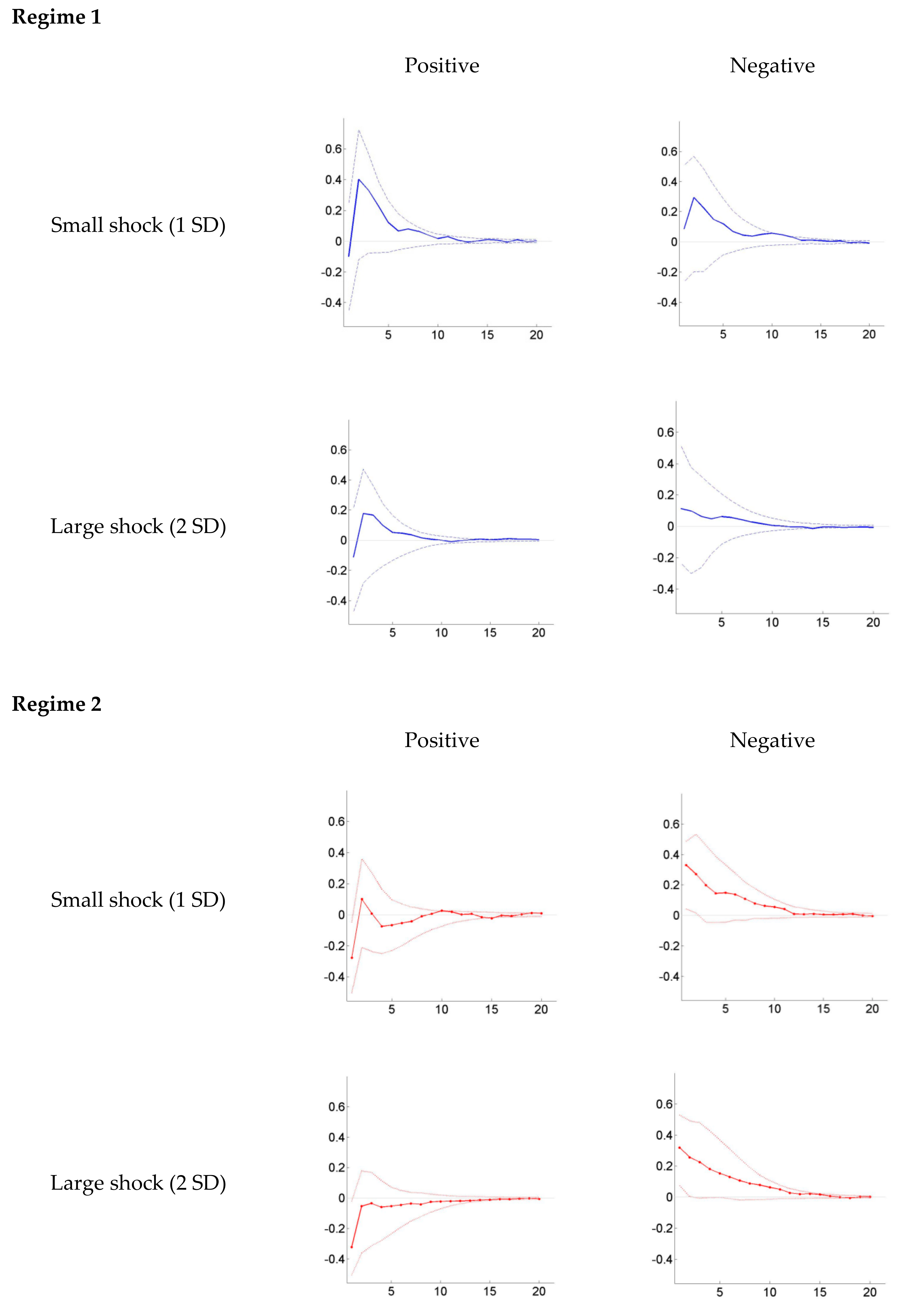
Figure 1,
Figure 2,
Figure 3 and
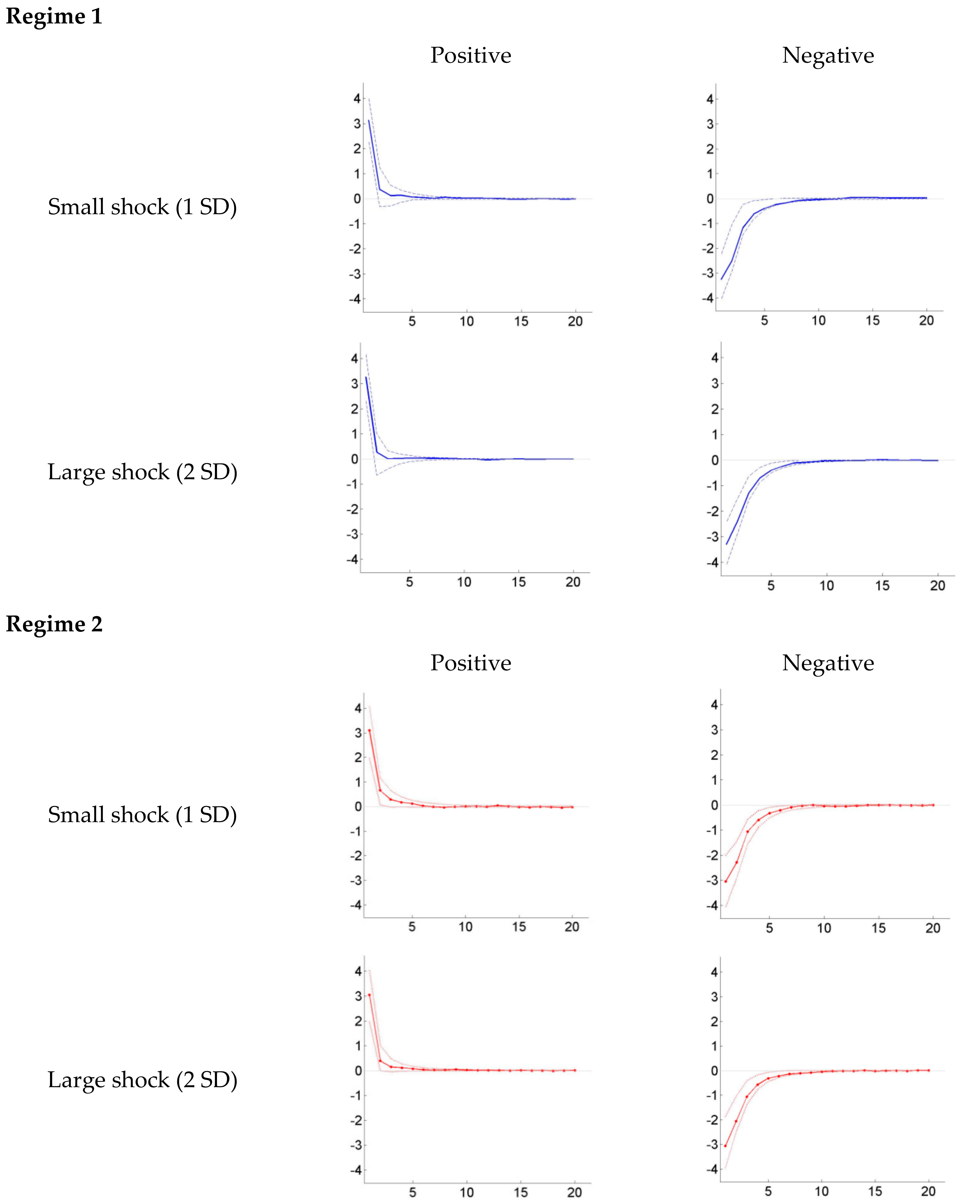
Figure 4 show the impulse responses of the current account, capital (financial) account, exchange rate volatility and short-term interest rate (Model 1) to the reserve shocks, dependent on whether the system is initially in the low regime or high regime, using exchange rate volatility as a threshold variable. The responses of these variables to four types of reserve shocks, which are a positive one-standard-deviation shock, a negative one-standard-deviation shock, a positive two-standard-deviation shock, and a negative two-standard-deviation shock, are presented. All generalized IRFs are scaled to correspond to one-standard-deviation (+1 SD or –1 SD) shocks to facilitate the comparison of impulse response functions. The values of these generalized impulse responses are summarized in the
Appendix A.
The current account shows no significant responses to positive and negative changes in reserves in Regime 1, which is the regime of low exchange rate volatility. However, when the system is initially in a high exchange rate volatility regime, an increase (decrease) in foreign reserves leads to a decrease (increase) in Korea’s current account. Specifically, the ratio of the current account to GDP declines (rises) by 0.3–0.35 pp in response to +1 SD (−1 SD) reserve-to-GDP shocks, regardless of the magnitude of the shocks. These responses, however, are only significant for a period of 1 to 2 months.
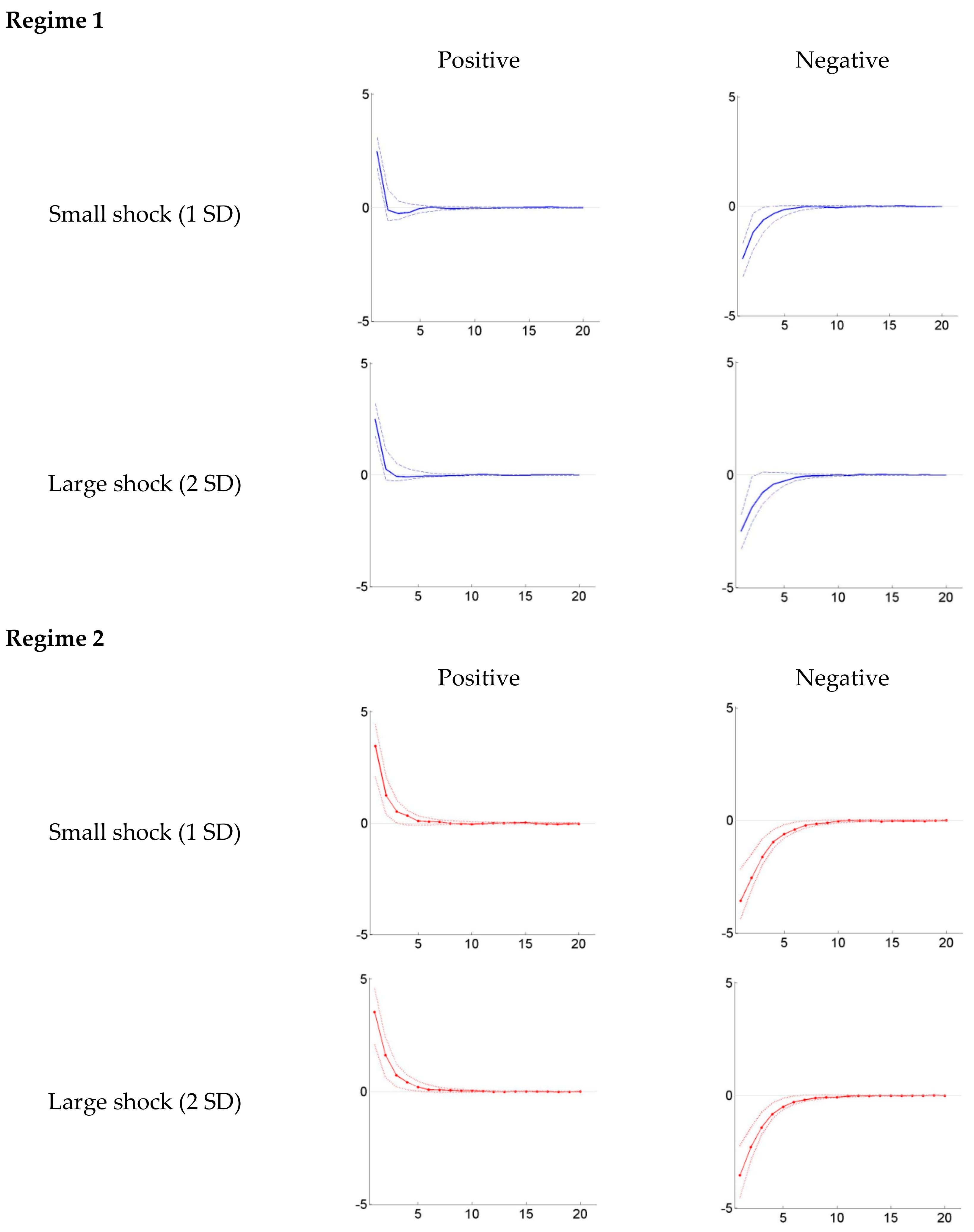
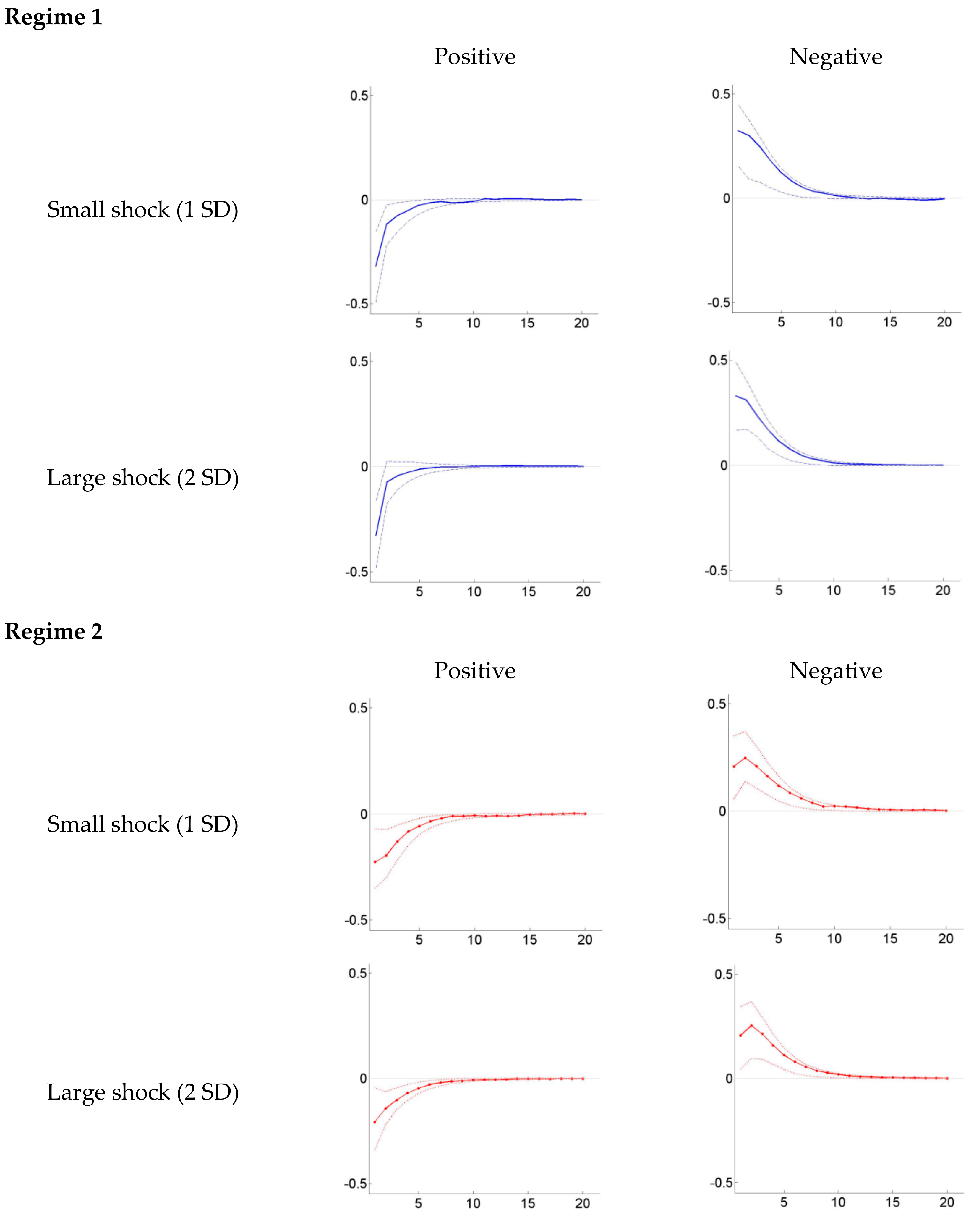
The capital (financial) account, on the other hand, is positively (negatively) affected by a positive (negative) shock to the ratio of reserves to GDP. We also observe asymmetries in the responses of the capital (financial) account depending on the regime the system is initially in. In Regime 1, a +1 SD (-1 SD) reserve shock is followed by a rise (fall) of approximately 2.5 pp in the ratio of the capital (financial) account to GDP. The capital (financial) account’s responses are stronger, at the 3.5–4 pp level, when the system is in the high exchange rate volatility regime. Furthermore, these responses last longer, remaining 5–7 months after the shocks.
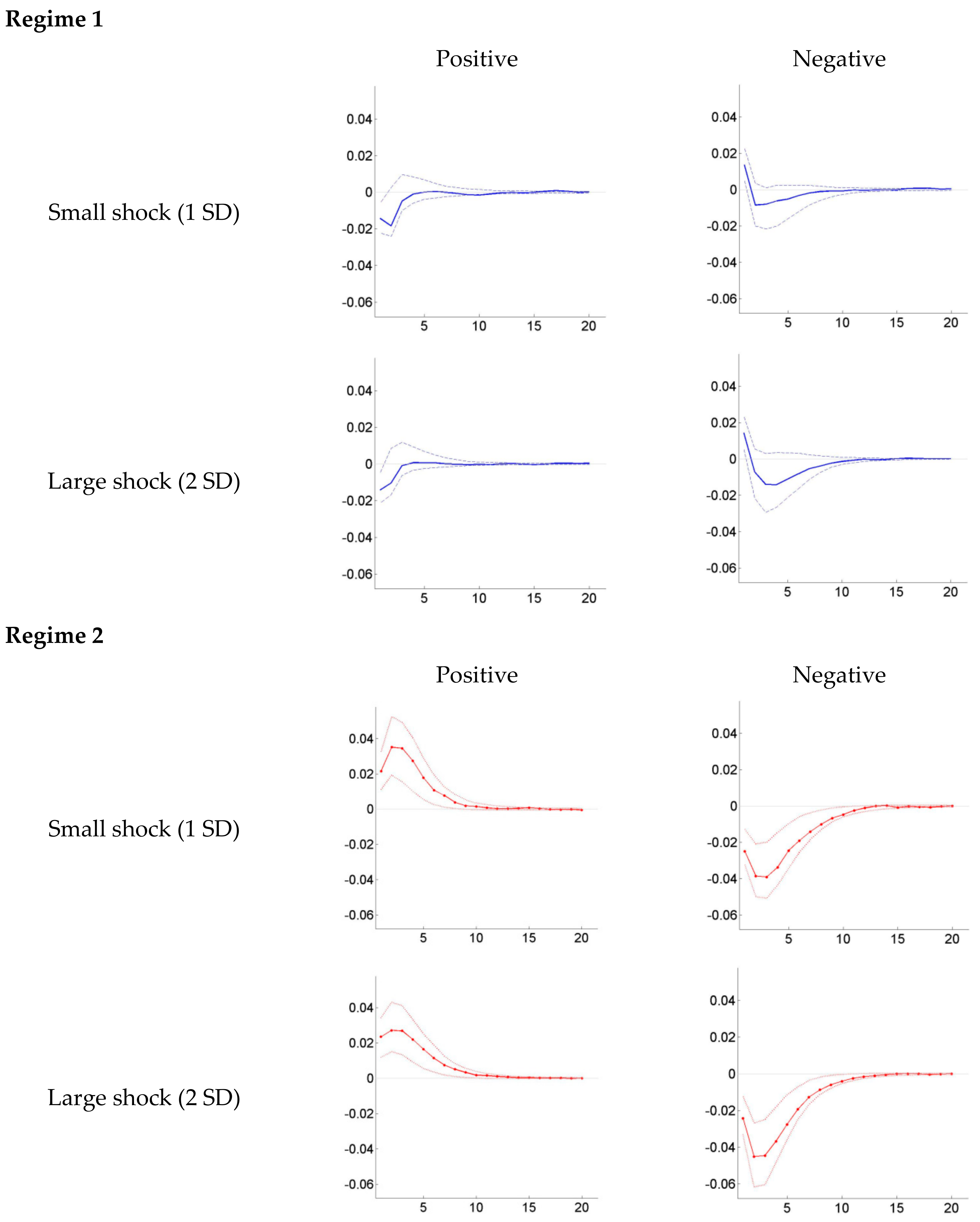
The exchange rate volatility is observed to significantly decrease (increase) by approximately 0.35 pp in response to a positive (negative) shock to the ratio of reserves to GDP when the system is in the high exchange rate volatility regime, while it is nonsignificant in the low regime.
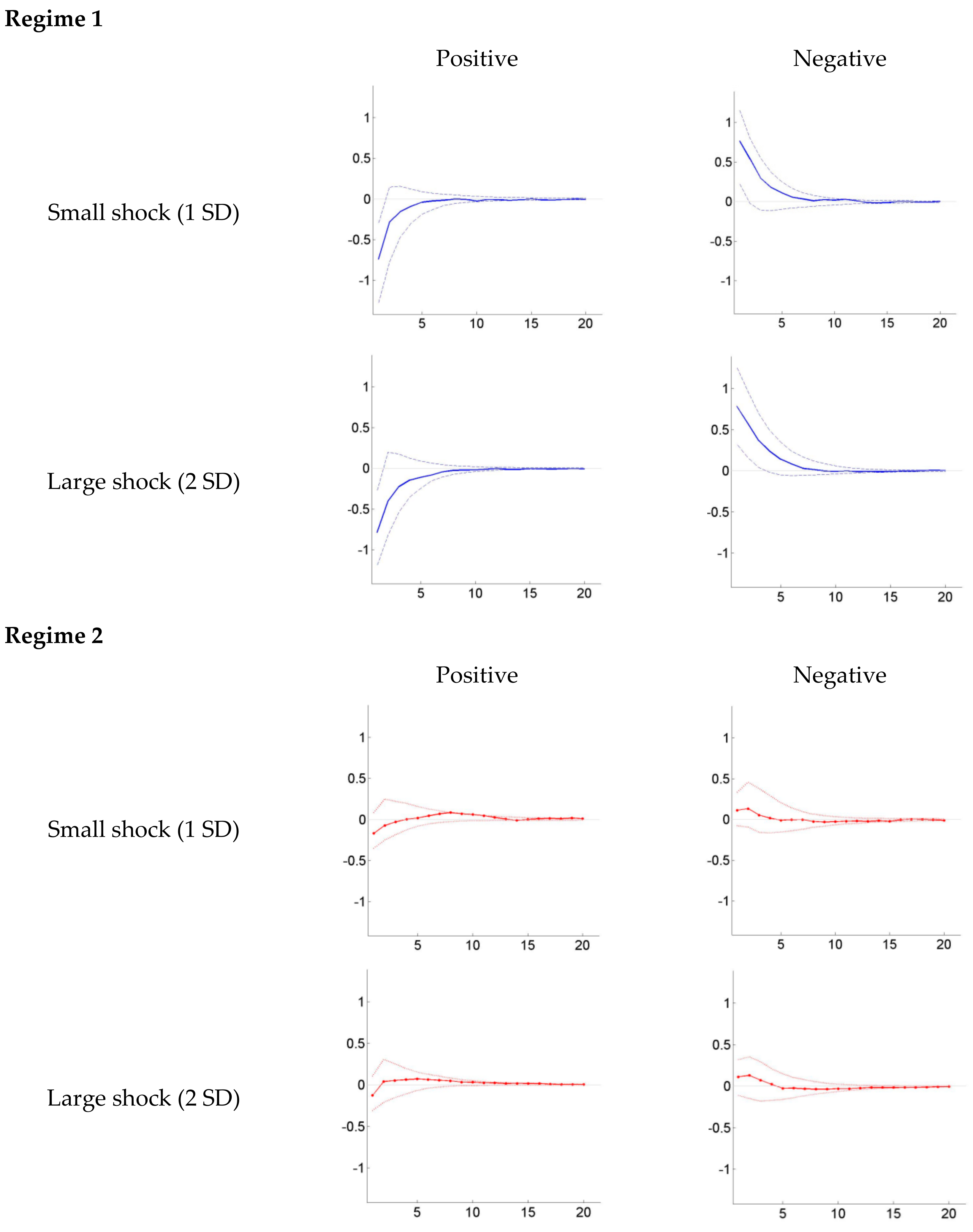
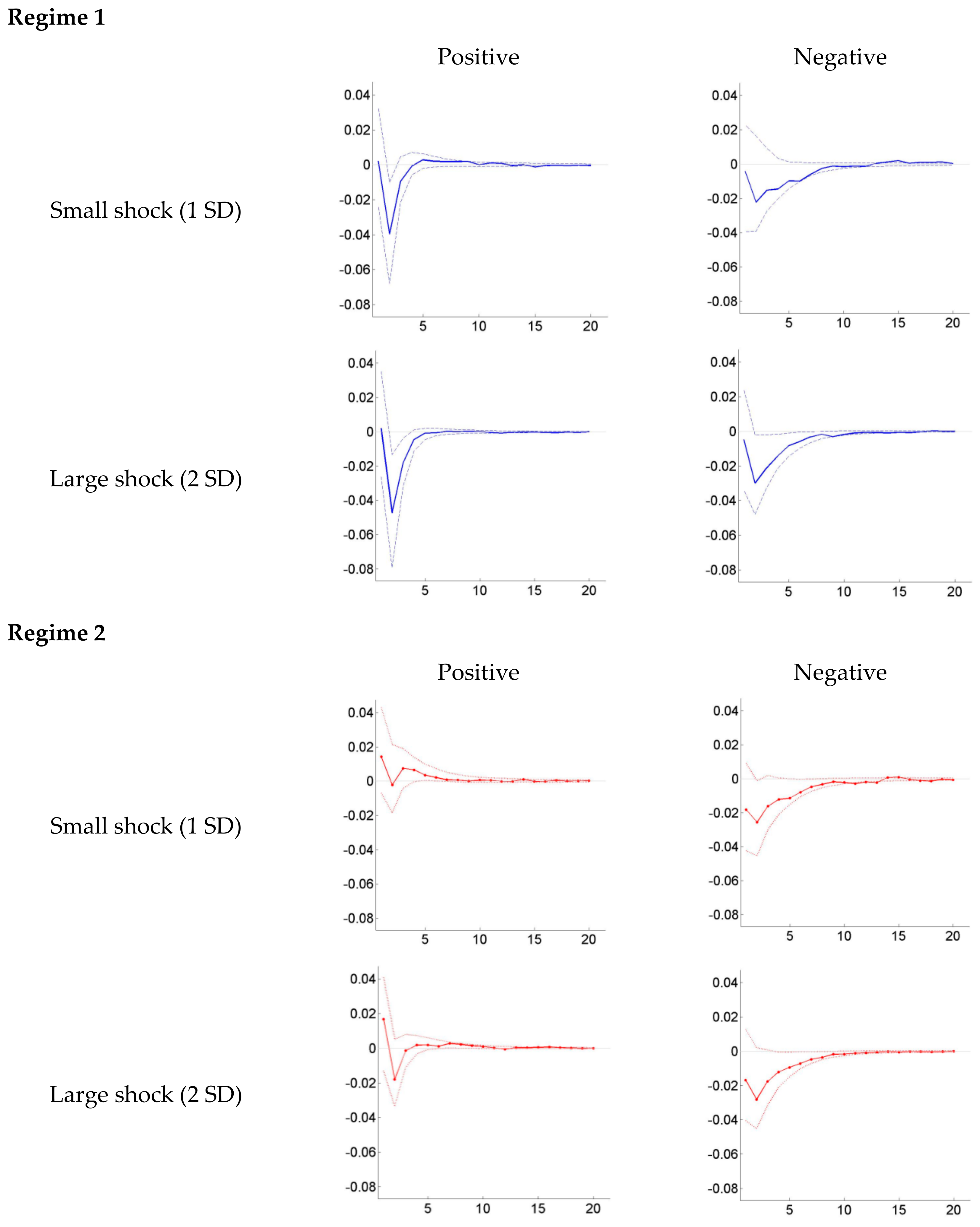
The responses of the short-term interest rate are more significant when the system is in the high exchange rate volatility regime. When analyzing the responses to the different types of shocks, Korea’s call rate is observed to respond differently according to the magnitude of the shocks. A positive (negative) one-standard-deviation reserve-to-GDP shock leads to a rise (fall) of 0.01 pp in the short-term interest rate. However, when the size of shock is adjusted to two standard deviations, the interest rate’s response to a negative shock is almost two times stronger than its response to a positive shock.
In Model 2 using the long-term interest rate, the current account’s responses to reserve shocks appear to be more significant when the system is initially in a regime with low exchange rate volatility. The ratio of the current account to GDP decreases (increases) by approximately 0.7 pp in response to a +1 SD (−1 SD) shock in Korea’s foreign reserves. Moreover, the reactions of the current account in the high regime are seen to be nonsignificant.
The responses of the capital (financial) account are consistent with Model 1’s results in general. However, we can see the symmetry of the capital (financial) account’s responses to the reserve shocks in this model, regardless of the regime the system is initially in or the direction and magnitude of the shocks.
The exchange rate volatility is observed to significantly respond to the shocks in foreign reserves in both the high and low exchange rate volatility regimes. A decrease (increase) of 0.2–0.3 pp in exchange rate volatility is recorded in the first month after the shock and lasts until the 7th month.
However, unlike the short-term interest rate, Korea’s long-term interest rate does not seem to be significantly affected by changes in foreign reserves. In both regimes, the 3-year government bond interest rate hardly shows any sign of a significant response, which is also fairly understandable, as the changes in reserve holdings are usually regarded to affect the short-term interest rate rather than the long-term interest rate.
5. Conclusions
Because South Korea is a small open economy, foreign trade makes up a large share of its GDP, which implies that the stability of the exchange rate is beneficial to safeguarding macroeconomic operations. In addition, to coincide with its domestic monetary policy or to contain abnormal fluctuations in the domestic exchange rate, the Bank of Korea (BOK) frequently intervenes in the forex. While the effects of intervention cannot be lumped together, we proceed with the empirical analysis based on a threshold vector autoregression (TVAR) model. TVAR is a feasible approach for classifying exchange rate volatility into high and low regimes by estimating threshold values. Under each regime, both the direction and the magnitude of the intervention are further taken into account. They shed light on the impact of foreign exchange intervention on various macroeconomic indicators in diverse circumstances.
Summarizing the results of model one intervention, under the low volatility regime, it had an effect on the capital (financial) account and the short-term interest rate, the former positively correlated and the latter negatively correlated with the direction of the shock. Albeit to varying degrees, all variables are subject to the influence of intervention under the high-volatility regime. It is noteworthy that the short-term interest rate is positively correlated with the initial status of the intervention, and the significant responses last longer in the high-volatility regime than in the low-volatility regime. Additionally, the responses of the capital (financial) account to reserve shocks vary across the regimes in terms of magnitude. For model 2, in comparison with the low-volatility regime, the responses of the current account to reserve shocks are no longer significant under the high-volatility regime. Taken together, we shed light on the fact that there are asymmetric effects of intervention. This provides a theoretical foundation for further application to other aspects of FXIs, such as timing, frequency, scale and method.


