Article

Developing a Forecasting Model for Real Estate Auction Prices Using Artificial Intelligence

1
Graduate Program in Investment Information Engineering, Yonsei University, Seoul 03722, Korea
2
Department of Industrial Engineering, Yonsei University, Seoul 03722, Korea
3
Department of Business Administration, Sejong University, Seoul 05006, Korea
*
Author to whom correspondence should be addressed.
Sustainability 2020, 12(7), 2899; https://doi.org/10.3390/su12072899
Submission received: 2 March 2020 / Revised: 31 March 2020 / Accepted: 2 April 2020 / Published: 5 April 2020

Abstract

:
The real estate auction market has become increasingly important in the financial, economic and investment fields, but few artificial intelligence-based studies have attempted to forecast the auction prices of real estate. The purpose of this study is to develop forecasting models of real estate auction prices using artificial intelligence and statistical methodologies. The forecasting models are developed through a regression model, an artificial neural network and a genetic algorithm. For empirical analysis, we use Seoul apartment auction data from 2013 to 2017 to predict the auction prices and compare the forecasting accuracy of the models. The genetic algorithm model has the best performance, and effective regional segmentation based on the auction appraisal price improves the predictive accuracy.

1. Introduction

In the past, the real estate industry was not recognized as an advanced industrial category. However, as a result of the informatization of the real estate industry and the linkage with financial markets, markets in financial investment instruments, such as real estate funds, Real Estate Investment Trusts (REITs) and Non-Performing Loans (NPL), have become active. Accordingly, many experts view the real estate industry as a financial field that is being explored more actively than in the past using artificial intelligence methods. A special feature of the real estate industry, the real estate auction market has played a key role in the industry’s development. Borrowers, lenders and investors are deeply involved in the real estate auction market, and the importance of the real estate auction process is increasing in the areas of finance and investment.
From January 2001 to December 2017, approximately 6.6 million real estate auctions were held in Korea nationwide, and the number of successful auctions, i.e., the number of sales, reached 2 million, while the average auction sale price rate was more than 71% of the appraisal value. Among regional markets, Seoul and the Gyeonggi province are the most active markets. The average auction sale price rate and the number of bidders in both markets are higher than the respective figures for the nationwide market. Especially looking at the apartment transaction market in Seoul, 692,397 private auctions, as well as 9435 institutional auctions, have been traded from January 2013 to December 2017. In this study, we use the data of the institutional apartment auction, which accounts for a high proportion of the total auctions in Seoul from January 2013 to December 2017. The data in the real estate auction industry are well-organized, enabling various in-depth analyses.
Considering both the real estate auction market and the capital market, the importance of related studies can be recognized. A real estate fund, which is a combination of real estate and finance, is structured to enable cooperation of many institutional participants, such as financial institutions, asset management companies and real estate management companies. This fund is a successful representative model that brought real estate to advanced financial markets; as of 2017, real estate fund assets amounted to more than 118 trillion Korean won, having grown by approximately 20% year-on-year. In other words, the real estate fund market has been expanding consistently with the growth of the capital market. For a more accurate investment in and management of this market, it is clear that there is a need for more studies of real estate using advanced techniques of data analysis and forecasting.
In this paper, we develop a forecasting model for real estate auction prices to provide forward looking auction market investors with useful information for future auction price prediction. We perform empirical analysis using artificial intelligence techniques with Korean auction market data. A recent study by Kang et al. [1] performed a chaos analysis of real estate auction sale price in Korean auction markets and confirmed that real estate auction sale price data has a deterministic structure. Therefore, it is worthwhile to develop forecasting models for real estate auction prices using various methodologies. Based on the result of Kang et al. [1], we construct forecasting models for real estate auction sale prices using artificial intelligence and a traditional statistical method; subsequently, we compare the predictive accuracy of models to identify the best model and optimization method. The artificial intelligence methods include a genetic algorithm (GA) and an artificial neural network (ANN); a statistical method of regression analysis is also used. This study is the first to consider forecasting the prices of individual real estate items using artificial intelligence methods.
The GA model is found to have the best performance. We also find that effective regional segmentation based on the auction appraisal price plays a key role in increasing the predictive accuracy of a forecasting model. These results offer valuable implications to forward looking investors at real estate auction markets, as well as managers of real estate funds. They are able to make more efficient investment strategies by using our GA model, which results in sustained economic benefits to the related stakeholder of real estate auction markets and the national economy. In this sense, the model developed in this study plays a role in sustaining economic growth.
The remainder of this paper is organized as follows. A literature review is presented in Section 2. The details of the model architecture are described in Section 3. In Section 4, the empirical analysis and results are presented. Finally, Section 5 presents the study’s conclusions.

2. Literature Review

There are several previous studies related to real estate forecasting using artificial intelligence, mostly with ANN and statistical analysis. Stevenson et al. [2] examined residential sale mechanisms from an appraisal perspective and empirically tests for differences in the valuation process for auctioned and private treaty sales. They tested the hypothesis that agents use different criteria in preparing the guide prices for auctioned housing, with an element of underpricing in order to aid in the marketing of the property and found agents do adjust valuations for auctions to attract additional potential bidders. In the 1990s, mass appraisal studies of real estate, especially residential property, have been performed using ANN [3,4,5,6,7,8]. Worzala et al. [9] applied neural network technology to real estate appraisal and compared the performance of two ANN models in estimating the sales price of residential properties with a traditional multiple regression model. They were concerned about the consistency and repeatability of results and the “black box” nature of neural networks in general. Results of the study did not support previous findings that ANNs are a superior tool for appraisal analysis. Nghiep and Al [10] predicted housing values using multiple regression analysis (MRA) and ANN, and compared the predictive power of models. The researchers showed that ANN performed better than MRA when a moderate to large data sample size was used. Limsombunchao [11] analyzed two models, the hedonic price model and ANN, for housing price prediction using a randomly selected sample of 200 houses in Christchurch, New Zealand. Factors, including house size, age and type, the number of bedrooms, bathrooms, garages, and amenities around the house, as well as geographical location, were considered in the study; the result showed the potential power of ANN to predict housing prices. McCluskey et al. [12] examined the comparative performance of an ANN and several multiple regression models in terms of their predictive accuracy in the mass appraisal industry. They found that a non-linear regression model had higher predictive accuracy than the ANN and the output of the ANN was not sufficiently transparent to provide an unambiguous appraisal model. McCluskey et al. [13] assessed a number of geostatistical approaches relative to an ANN model and the traditional linear hedonic pricing model for mass appraisal valuation. They found that ANNs outperformed the traditional multiple regression models and approached the performance of spatially weighted regression models. However, ANNs retain a “black box” architecture that limits their usefulness to practitioners in the field. A relatively recent study by Núñez Tabales et al. [14] insisted on the use of ANN if there were enough statistical information and an extensive set of data spanning years. The authors considered exogenous variables and factors, such as buildings located nearby and surroundings of a house. Zhou et al. [15] tried to improve existing ANN-based prediction models and finally presented several suggestions for a mass appraisal of real estate in China.
In addition to ANN-based studies, there are several previous studies of real estate prediction using GA. Ahn et al. [16] used ridge regression with GA (GA-Ridge) to enhance real estate appraisal forecasting. The researchers performed an experimental study of the Korean real estate market and verified that GA-Ridge was effective in forecasting real estate appraisals. Del Giudice et al. [17] used GA to interpret the relationship between real estate rental prices and geographical locations of houses, and compared the results of GA and MRA to verify the potential forecasting power of GA.
Only a small number of similar studies of the Korean real estate industry have been performed. Han [18] attempted to construct a forecasting model for real estate appraisal price using GA ridge regression and compared the model to ANN and multiple regression. The study is meaningful in that it forecast a time series index related to the Korean real estate industry with a macroeconomic indicator and tried to use artificial intelligence methodologies. Kwon [19] researched a nonlinear macroeconomic time series forecasting model and is one of the empirical studies that forecast real estate prices. Unlike the past real estate forecasting models based on macroeconomic indicator data, this study designed an artificial housing market and applied GA with agent-based modeling (ABM). Chung [20] tried to construct a forecasting model for the apartment price index using ANN. The model forecast time series using the real estate price index and macroeconomic data, but had a limitation because it included a small number of variables.

3. Model Architecture

The purpose of this study is to develop forecasting models for the auction sale price. For this purpose, GA, ANN and a regression model are used (see Figure 1). In particular, this study focuses on forecasting prices of individual real estate auction items. To estimate these individual prices, sufficient data needs to be collected to construct forecasting models effectively. In addition, aspects, such as how to subdivide the analysis area (the area of Seoul in this paper) are very important.

3.1. Data Selection

The data for this study covers real estate auction cases of apartments in Seoul for the preceding five years. The data are collected from real estate auction information companies, banks, statistical offices and other related organizations. To remove insignificant factors that may pose obstacles to experiments, the results of previous studies regarding the key factors of real estate auctions are considered before an empirical study. As the format and scale of collected data vary, a standardization process is also required. The training set for constructing models and a separate testing set are assigned approximately 70% and 30%, respectively, of the entire size of data.

3.2. Grouping Process

In this step, several grouping processes for data are applied, and forecasting models are constructed for each group independently to compare the results. Theoretically, the performance will improve if the similarity within a group increases and that between groups decreases. The Seoul area is divided into 25 boroughs, which is the most segmented separation. Afterwards, grouping criteria according to the 2020 Seoul City Basic Plan are applied based on administrative and residential areas. The plan divides Seoul into five zones: The urban zone, and southeast, northeast, southwest and northwest zones (see Table 1). Finally, another model is constructed using clustering based on auction appraisal prices. Based on the average auction appraisal price of each borough, all 25 boroughs are classified into several groups using the cluster analysis [21,22,23,24]. This process can be effective for improving model performance because auction appraisal price is one of the most important factors associated with a real estate auction. In other words, the classification based on auction appraisal price can increase homogeneity within groups and heterogeneity between groups [25,26,27].

3.3. Regression Model

A linear regression model determines the characteristics and relationship between independent variables and a dependent variable. A simple linear regression model incorporates one independent variable, while a multiple linear regression model incorporates multiple independent variables [28,29,30]. The linear regression analysis estimates the following linear equation that describes a plane that passes closest to each data point on a scatter plot.
Y n = a 1 x 1 + a 2 x 2 + + a p x p + ε n
This equation incorporates p independent variables. From this equation, a 1 ,   , a p , coefficients of independent variables x 1 ,   , x p , are estimated to forecast y n given independent variables x 1 ,   , x p . In this paper, the forecast value is the auction sale price, and the independent variables are selected from the real estate auction procedure and macroeconomic data. In the process of estimating the coefficients, the sum of squared errors (SSE) for a linear equation is minimized; this approach is called the method of least squares [31,32,33].

3.4. Artificial Neural Network

ANN is a technique that reproduces humans’ intelligent activities [34,35,36]. An ANN model capable of expressing nonlinear relations has attracted attention as an approach to overcoming the limitations of the traditional statistical methodologies that express forecasting models through linear combinations of independent variables. The model mimics human brain cells and does not assume any linear distribution of probabilities or variables. Therefore, ANNs can be used for more varieties of data than can be traditional statistical methods [37,38,39].
An ANN consists of nodes and weights. A collection of nodes with similar properties is called a layer; typically, there are three types of layers: Input, hidden and output [34,35,36,37,38,39]. The input layer consists of input nodes that accept input values of data. The hidden layer consists of hidden nodes; each node of the hidden layer accepts output values of the previous layer as input values. The output layer consists of output nodes that represent the final output values of the network. The nodes of different layers are connected by their respective weights that are multiplied when output values of nodes are passed to other nodes. Every node of the network computes the output values by applying an activation function to input values. There are various activation functions, and we use the following sigmoid function;
f ( x ) = 1 1 exp ( x )
There are various ANN architectures, but the multi-layer perceptron is the most efficient. Multi-layer perceptron is a neural network with one or more hidden layers between the input layer and output layer. In the input layer, input data is received from the outside of the system and transmitted to the system. The hidden layer located inside the system takes input values, processes them, and generates the results. The output layer calculates the system value based on the input value and the current system state (see Figure 2). In this paper, we use the multi-layer perceptron with two hidden layers.

3.5. Genetic Algorithm

GA is an optimization methodology presented by Holland [40,41]. To search for the optimized solution, a GA uses the principles of Darwinian evolution that consists of crossover, selection and mutation [42,43]. Before searching for the optimal solution, the method represents the solutions as a binary data structure called a chromosome, and a set of chromosomes is called a population. Then, by implementing the algorithm, the fitness values of solutions increase until the specifically designated conditions are satisfied. The fitness value is calculated by the fitness function initially established to illustrate the goal of the problem. The entire process of a GA searching for the optimal solution is shown in Figure 3.
Selection is the operation of selecting two parent solutions that are more appropriate than others to determine the composition of the offspring generation based on the survival principle of the natural system. In general, chromosomes are selected with probability proportional to their fitness or from top to bottom in descending order of fitness ranking. One should choose the solution with the higher fitness. As the process of selection is repeated, it is expected that inferior solutions will be reduced, and superior solutions will survive through the generations.
Crossover is a representative operation of a GA. Crossover is a method for generating a new offspring through mixing genes in the parent chromosomes. Generally, two parent chromosomes are cut by the number of specific points, and the cut parts are exchanged with each other. In the uniform crossover, genes at randomly selected positions of one parent are exchanged with those of another parent. Using various crossover methods, the good genetic information of chromosomes of the previous generation can be preserved, and more optimized chromosomes than those observed in the past can be searched for simultaneously.
The mutation is a way to construct a new direction for finding a solution using the birth of a totally new offspring (chromosome). Crossover can bind genes in a good direction; however, it is difficult to introduce new genes that are not from parental traits. Mutation can create new chromosomes that are better than those observed in the past by randomly replacing a certain value of genes in chromosomes that already exist. However, due to randomness, crossover implies a risk of producing inferior chromosomes. By repeating these processes until the specified requirements are satisfied, the generation progresses, and the fitness of chromosomes (solutions) is improved.
In this paper, GA is used to search for the optimized values of a regression model that predicts the real estate auction price after a period of time [44,45]. The GA stops when a number of generations have all evolved. The larger the population and generation, the greater the likelihood that a globally optimized solution will be obtained, but the complexity of finding optimal variables will increase exponentially. Therefore, the empirical analysis is usually carried out using a reasonable stopping condition in the process of finding an optimal solution. In this paper, the optimization process ends when the average population fitness does not improve, or the surviving chromosomes do not change after 20,000 iterations. The main parameters of the GA, such as population size, crossover rate, and mutation rate, are set to 50, 0.5, and 0.05, respectively, which are commonly used default settings. The optimized values serve as regression coefficients. The objective function of the algorithm for this model is shown by (3).
Objective   Function = 1 n i = 1 n | F i Z i Z i |
where F I represents the forecast values, and I is the real-world value of i-th property.

4. Empirical Analysis

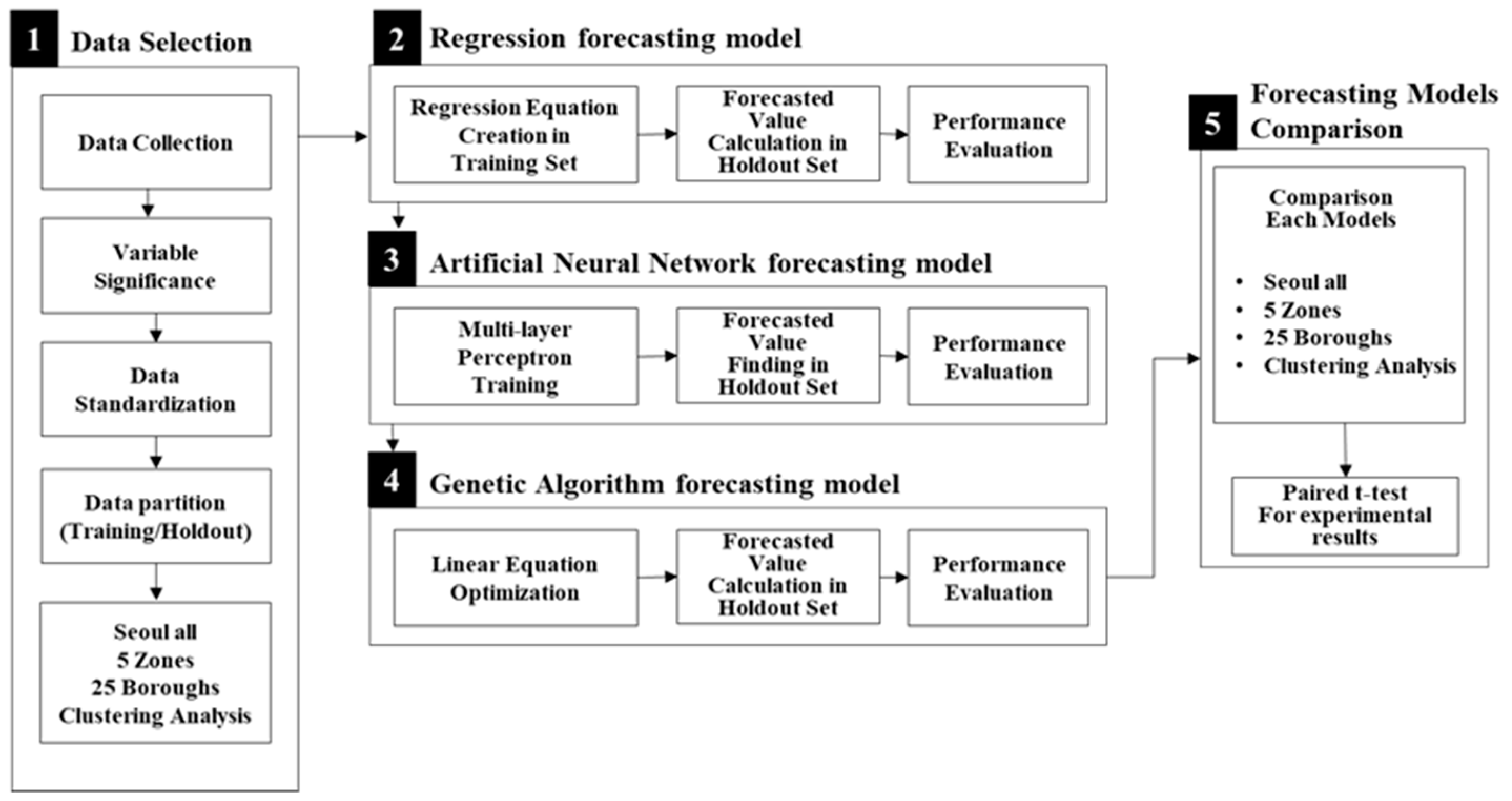
4.1. Data and Methodology

In this study, the auction data collected from the GG Auction Co., Ltd., Infocare Auction Co., Ltd., Bank of Korea, Kookmin Bank, Statistics Korea (KOSTAT) and Korea Exchange (KRX) were used for the empirical study. The number of data points is 9435, and the sample period of data is from January 1, 2013, to December 31, 2017. The data covers all the apartment auction items in Seoul for over five years. The reason for analyzing the Seoul area is that apartment prices in Seoul are more standardized than those in other areas.
Many previous studies of the Korean real estate industry have been limited to time series analysis of real estate prices and indices. In contrast, this study focuses on forecasting the individual prices of real estate auction items. Therefore, it is necessary to reduce the volatility of the value to be forecasted by using large amounts of data and appropriate variables. The variables affecting the real estate auction price are approximately divided into three categories: Auction characteristics, the physical properties of the real estate, and macroeconomic variables (See Table 2).
The variables classified as auction characteristics include appraisal price, average auction sales price rate, average number of bidders, number of bids, number of views, auction period, and auction index. These variables are considered important in this study because a real estate auction is the only system based on the laws of Korea, and hence, the auction characteristics inevitably have a significant impact on the auction price.
The variables classified as physical properties include exclusive area, land area, land portion, unpaid management fee, tenant, lien, priority lease, legal superficies, fractional right auction, dependent right, special right, school distance, bus stop, and subway distance. In addition, some of these the variables are classified as macroeconomic data, as shown in Table 2.
Real estate has strong individual characteristics depending on the physical, legal and economic values that differentiate properties of real estate in the same area. Therefore, the variables listed in Table 2 can be key factors that determine the prices of real estate. The detailed descriptions of all used variables and their source are shown in Table 3.
Before conducting the experiment, standardization is needed because the type and scale of collected data vary. Standardization is the process of adjusting the values of each variable to a range from 0 to 1. This type of data preprocessing is known to be efficient for model construction and forecasting [46,47]. In this study, the min-max standardization method is used, as defined by Equation (4). To derive the forecast values, this formula is rearranged, as shown in Equation (5).
Standardization value = (Real value − Min) / (Max − Min)
Forecast value = Forecast ratio × (Max − Min) + Min
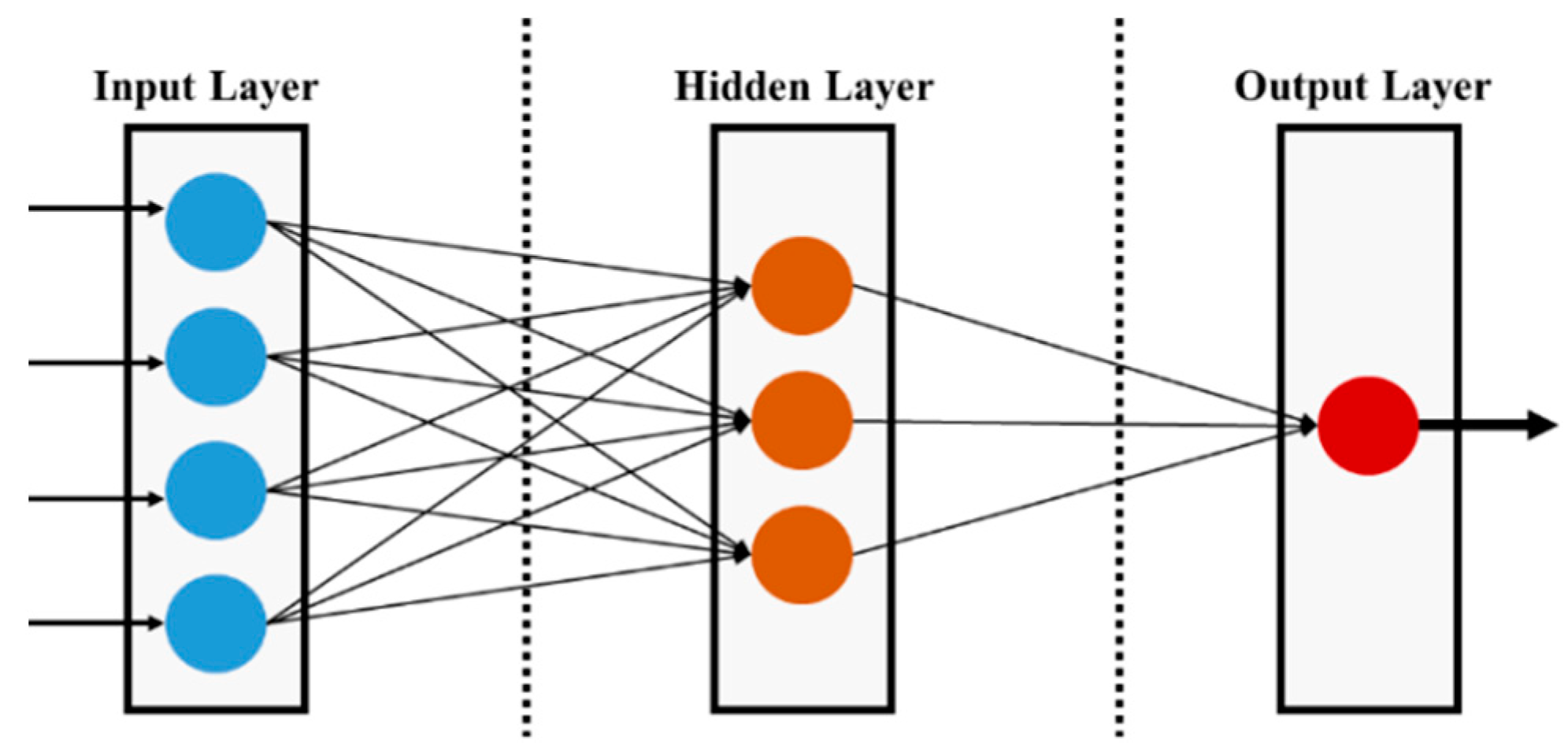
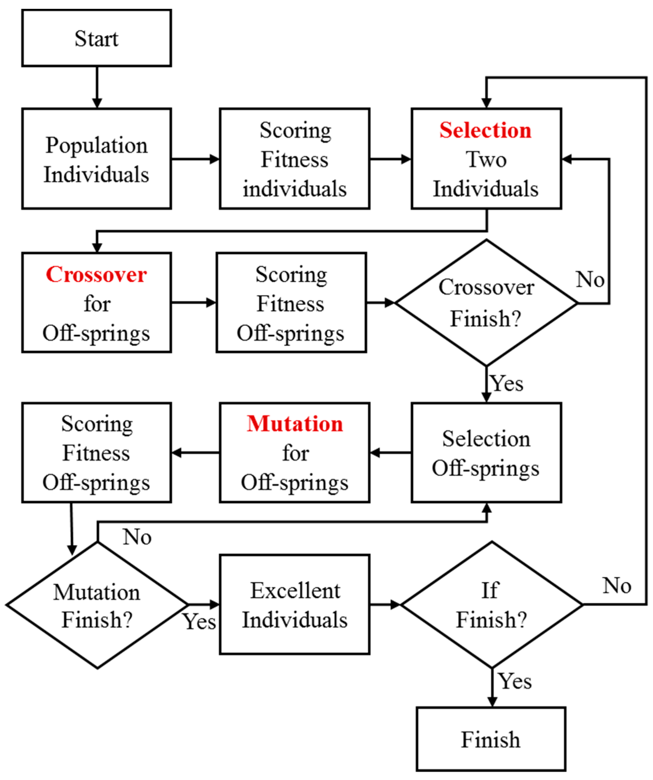
To develop a multiple regression model, all variables are included in the model. In the case of the ANN model, there are two hidden layers and 60 hidden nodes in each layer. The sigmoid function is adopted as the activation function because we want to forecast values between 0 and 1. Finally, coefficients in the linear regression model are optimized. For a GA model construction, the number of trials, population size, crossover rate, and mutation rate is set to 20,000, 50, 0.5 and 0.05, respectively.
The performance of models is measured by the mean absolute percentage error (MAPE), and root mean square error (RMSE) calculated by Equations (6) and (7), respectively.
M A P E = 1 n i = 1 n | P i F i P i |
R M S E = i = 1 n ( P i F i ) 2 n
where P i and F i are, respectively, the real-world and forecast auction sale prices of i-th real estate, and the number of auction items is n. Without the grouping process, the training and holdout sets are composed of 6568 and 2867 auction cases, respectively. They are randomly chosen from all auction cases in Seoul.

4.2. Empirical Results

Table 4 shows the results of the proposed forecasting models using data without the grouping process. The results in Table 4 show that the GA model (MAPE is 8.86 and RMSE is 0.006) has the best performance on the holdout set among the three models.
To measure how close the forecast values are to market values, the average forecast of auction sale price rate is compared to the average of market auction sale price rate. The auction sale price rate means the ratio of the auction sale price to the auction appraisal price, calculated by Equation (8).
A u c t i o n   s a l e   p r i c e   r a t e = A u c t i o n   s a l e   p r i c e A u c t i o n   a p p r a i s a l   P r i c e ,
As the auction appraisal price is fixed, the forecast price is sufficiently close to the market price if the average forecast of auction sale price rate is similar to that of market auction sale price rate. Table 5 reports the average of market auction sale price rates and the average forecast of auction sale price rate obtained using regression, ANN and GA models. As shown in Table 5, the annual average forecast of auction sale price rates from the GA model is approximately estimated to be 83% in 2013, 87% in 2014, 93% in 2015, 93% in 2016, and 97% in 2017. These results are very close to the annual average of market auction sale price rates. In addition, the average value of the forecast auction sale price rate resulting from the GA model (0.9040) is observed to be closer than the respective values of other models to that of market auction sale price rate (0.9306).
In the next step, several grouping processes are performed to improve forecasting performance. At first, grouping according to five zones based on the 2020 Seoul City Basic Plan is used. The five zones consist of urban, southeast, northeast, southwest and northwest zones. The number of auction cases in each zone is 475 in the urban zone, 2143 in the southeast zone, 3113 in the northeast zone, 2771 in the southwest zone, and 933 in the northwest zone. The ratio of the training and holdout sets is the same as in the previous experiment. Table 6 reports the MAPE and RMSE of the proposed forecasting models applied to the holdout set with the grouping process based on five zones.
The results in Table 6 show that the MAPE and RMSE of the GA model are the lowest among the values of the three forecasting models in all five zones of Seoul. The average values of MAPE and RMSE of the GA model for five zones are 8.31 and 0.0047, respectively. This result implies an improvement over the previous experimental results without the grouping process. Note that the values of MAPE and RMSE of the GA model applied to the holdout set without the grouping process are 8.86 and 0.0060, respectively (see Table 4).
Table 7 reports the averages of market auction sale price rate and of forecast auction sale price rate obtained using regression, ANN and GA models for five zones. The GA model shows the best performance, i.e., the average auction sale price rate obtained with the GA model is the closest to that of market auction sale price rates in all five zones.
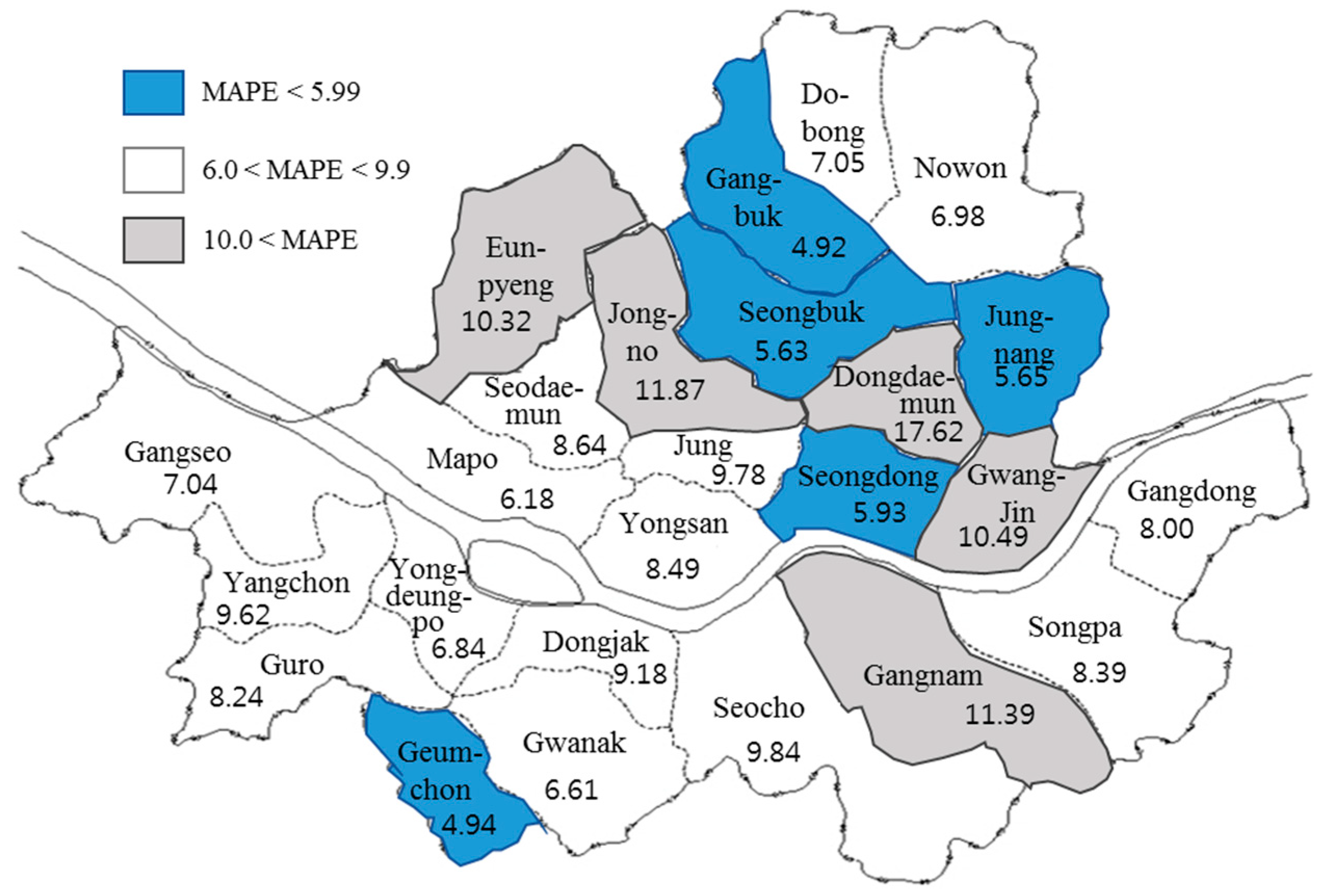
To group data more specifically, we perform the analysis for each of 25 boroughs independently. The forecasting errors in each borough for all three models are shown in Table 8. The GA model shows the lowest MAPE in all boroughs, whereas, the regression and the ANN model show lower values of RMSE than those of the GA model in some boroughs. On average, the GA model shows the best performance among three models with the lowest average values of MAPE (8.70) and RMSE (0.0040). Figure 3 shows the MAPE values of the GA model in 25 boroughs. In Figure 4, no regularity and homogeneity of MAPE are observed for boroughs. For instance, the GA model has a high forecasting power in Seongdong-gu (MAPE is 5.93) and a relatively poor forecasting power (MAPE is 17.62) in nearby Dongdaemun-gu. This result indicates that the auction market in each borough of Seoul has its unique characteristics.
Finally, the 25 boroughs of the Seoul area are grouped based on the auction appraisal price to reflect characteristics of the auction market. In this experiment, only the GA model is constructed because the GA algorithm is superior to others, as shown by both previous experimental results. The 25 boroughs are grouped into 3 to 6 groups in the descending order of the auction appraisal price, i.e., zone 1 is the group with the highest average auction appraisal price. The GA models are constructed for each group independently. Table 9 shows the segmentation of boroughs based on the auction appraisal price. The forecasting results of a GA model for every zone are reported in Table 10. The average MAPE (RMSE) in Table 10 indicates that the GA model with the six-group clustering based on auction appraisal price shows the best performance among other segmentation methods. The average MAPE (7.83) of the GA model with the six-group clustering based on auction appraisal price in Table 10 is observed to be superior to that based on 25 individual boroughs (8.70) in Table 8. This result implies that clustering based on appraisal price and constructing the GA forecasting models for each cluster improves the average performance. Accordingly, auction appraisal price is likely to play a more significant role in increasing homogeneity within a group of auction cases than that of locations of real estate. It is also noted that the MAPE and RMSE for zones classified as having lower auction appraisal prices are lower than those for zones classified as having higher auction appraisal prices in all segmentation methods. In other words, the lower the auction appraisal price is, the better the performance of the GA model is.
As the final step, we perform the paired t-test of the forecast values of all models to verify results from our experiments using various grouping processes. Table 11 shows p-values of the paired t-test for three forecasting models without a grouping process. The results indicate significant differences in performance by all pairs of models [16,30,48]. Similarly, the paired t-test for models with grouping based on five zones is performed. Results in Table 12 show that all zones except the northwest zone have significant p-values, implying a better performance of the GA model than that of other models. When we construct models with grouping based on 25 boroughs, results of the paired t-test are inconsistent. As shown in Table 13, the performance of models is not observed to be significantly different in some boroughs, whereas, significant differences are observed in other boroughs. Although the average performance of the GA model appears to be the best in Table 8, the grouping process based on 25 boroughs does not seem to improve the performance of the GA model in some groups.
As shown by our experimental results, the grouping process based on the auction appraisal price improves performance of forecasting models. In particular, classification into six zones shows the best performance. To verify the improvement of model performance by grouping based on auction appraisal price, we perform the paired t-test for the GA model with grouping data based on auction appraisal price and five zones of the 2020 Seoul Basic City Plan. Table 14 reports the results of this paired t-test. The p-values in Table 14 show that the forecasting ability of the GA models with grouping into 4, 5 and 6 zones based on auction appraisal price is significantly different from that with grouping based on five zones of the 2020 Seoul Basic City Plan. These results imply that the price-based variable is a more significant factor in improving the GA model performance than are variables related to administrative and living areas.

5. Conclusions

In this paper, we present three forecasting models for real estate auction sale price using artificial intelligence and statistical methodologies: A regression model and ANN and GA models. Our empirical study shows that the GA model has the best performance. In addition, three grouping processes are applied to improve the performance of the GA models. The GA model with grouping based on auction appraisal price is more efficient than all other forecasting models constructed in this paper. These empirical results imply that appropriate criteria for the grouping process play a key role in increasing the predictive accuracy of a forecasting model. They also offer valuable implications to forward looking investors at real estate auction markets, as well as managers of real estate funds.
Real estate industry has become an essential part of today’s financial markets. Nowadays, a number of researchers and practitioners have explored the real estate field using statistical and artificial intelligence techniques. To offer a comprehensive view of the auction markets, which is an influential sector of real estate industry, this study develops forecasting models to predict future prices of individual real estate auction items. To our best knowledge, this is the first study on using data of individual apartment auction prices to develop forecasting models for real estate auction prices. Real estate fund managers are able to make more efficient investment strategies by using our GA model. It contributes to the investment efficiency of the real estate auction markets and helps to achieve efficient financial markets. In addition, it helps to achieve sustained economic benefits to the related stakeholder of real estate auction markets. In this sense, the model developed in this paper plays a role in sustaining economic growth.
This study has potential limitations. The model developed in this study is based on the data of apartment auction markets in Seoul during the sample period. As such, the empirical results are limited to apartment auction markets in Seoul traded in a specific time period. Based on the idea of our model, future research can be enriched by developing a model that can be utilized for other real estate sectors. More improvement of forecasting ability and wider use of the models are expected with more diverse data. The study could also be extended by researching the key factors of the grouping process to improve model performance.

Author Contributions

Formal analysis, data curation, resources, funding acquisition, J.K.; conceptualization, methodology, project administration, K.J.O.; validation, investigation, writing—review and editing, H.S.L.; writing—original draft preparation, visualization, software, H.J.L. and S.H.J.; All authors have read and agreed to the published version of the manuscript.

Funding

This work is supported by GG Investment Management Co., LTD.

Conflicts of Interest

Authors declare no conflict of interest.

References

  1. Kang, J.; Kim, J.; Lee, H.J.; Oh, K.J. Chaos analysis of real estate auction sale price rate time series. J. Korean Data Inf. Sci. Soc. 2017, 28, 371–381. [Google Scholar]
  2. Stevenson, S.; Young, J.; Gurdgiev, C. A comparison of the appraisal process for auction and private treaty residential sales. J. Hous. Econ. 2010, 19, 145–154. [Google Scholar] [CrossRef]
  3. Do, A.Q.; Grudnitski, G. A neural network approach to residential property appraisal. Real Estate Apprais. 1992, 58, 38–45. [Google Scholar]
  4. Kathmann, R.M. Neural networks for the mass appraisal of real estate. Comput. Environ. Urban Syst. 1993, 17, 373–384. [Google Scholar] [CrossRef]
  5. Rossini, P. Artificial neural networks versus multiple regression in the valuation of residential property. Aust. Land Econ. Rev. 1997, 3, 1–12. [Google Scholar]
  6. Rossini, P. Improving the results of artificial neural network models for residential valuation. In Proceedings of the Fourth Annual Pacific-Rim Real Estate Society Conference, Perth, Australia, 19–21 January 1998. [Google Scholar]
  7. Rossini, P. Accuracy issues for automated and artificial intelligent residential valuation systems. In Proceedings of the International Real Estate Society Conference, Athens, Greece, 19 January 1999. [Google Scholar]
  8. Tay, D.P.; Ho, D.K. Artificial intelligence and the mass appraisal of residential apartments. J. Prop. Valuat. Invest. 1992, 10, 525–540. [Google Scholar] [CrossRef]
  9. Worzala, E.; Lenk, M.; Silva, A. An exploration of neural networks and its application to real estate valuation. J. Real Estate Res. 1995, 10, 185–201. [Google Scholar]
  10. Nghiep, N.; Al, C. Predicting housing value: A comparison of multiple regression analysis and artificial neural networks. J. Real Estate Res. 2001, 22, 313–336. [Google Scholar]
  11. Limsombunchai, V. House price prediction: Hedonic price model vs. In artificial neural network. In Proceedings of the New Zealand Agricultural and Resource Economics Society Conference, Blenheim, New Zealand, 25–26 June 2004. [Google Scholar]
  12. McCluskey, W.J.; Davis, P.T.; Haran, M.; McCord, M.; McIlhatton, D. The potential of artificial neural networks in mass appraisal: The case revisited. J. Financ. Manag. Prop. Constr. 2012, 17, 274–292. [Google Scholar] [CrossRef]
  13. McCluskey, W.J.; McCord, M.; Davis, P.T.; Haran, M.; McIlhatton, D. Prediction accuracy in mass appraisal: A comparison of modern approaches. J. Prop. Res. 2013, 30, 239–265. [Google Scholar] [CrossRef]
  14. Núñez Tabales, J.M.; Caridad y Ocerin, J.M.; Rey Carmona, F.J. Artificial neural networks for predicting real estate prices. Revista De Metodos Cuantitativos Para La Economía Y La Empresa 2013, 15, 29–44. [Google Scholar]
  15. Zhou, G.; Ji, Y.; Chen, X.; Zhang, F. Artificial Neural Networks and the Mass Appraisal of Real Estate. Int. J. Online Eng. (iJOE) 2018, 14, 180–187. [Google Scholar] [CrossRef] [Green Version]
  16. Ahn, J.J.; Byun, H.W.; Oh, K.J.; Kim, T.Y. Using ridge regression with genetic algorithm to enhance real estate appraisal forecasting. Expert Syst. Appl. 2012, 39, 8369–8379. [Google Scholar] [CrossRef]
  17. Del Giudice, V.; De Paola, P.; Forte, F. Using genetic algorithms for real estate appraisals. Buildings 2017, 7, 31. [Google Scholar] [CrossRef] [Green Version]
  18. Han, Y.C. Using Genetic Algorithm to develop Ridge regression for Real Estate Forecasting. Master’s Thesis, Yonsei University, Seoul, Korea, 2008. [Google Scholar]
  19. Kwon, B.C. An Empirical Study of a Nonlinear Forecasting Model for Macroeconomic Time Series. Ph.D. Thesis, Seoul National University of Science and Technology, Seoul, Korea, 2014. [Google Scholar]
  20. Chung, W.G.; Lee, S.Y. A Study on the Forecasting of the Apartment Price Index Using Artificial Neural Networks. Hous. Stud. Rev. 2007, 15, 39–64. [Google Scholar]
  21. Cheong, D.; Kim, Y.M.; Byun, H.W.; Oh, K.J.; Kim, T.Y. Using genetic algorithm to support clustering-based portfolio optimization by investor information. Appl. Soft Comput. 2017, 61, 593–602. [Google Scholar] [CrossRef]
  22. Hruschka, E.R.; Ebecken, N.F. A genetic algorithm for cluster analysis. Intell. Data Anal. 2003, 7, 15–25. [Google Scholar] [CrossRef]
  23. Nanda, S.R.; Mahanty, B.; Tiwari, M.K. Clustering Indian stock market data for portfolio management. Expert Syst. Appl. 2010, 37, 8793–8798. [Google Scholar] [CrossRef]
  24. Tola, V.; Lillo, F.; Gallegati, M.; Mantegna, R.N. Cluster analysis for portfolio optimization. J. Econ. Dyn. Control 2008, 32, 235–258. [Google Scholar] [CrossRef] [Green Version]
  25. Bansal, A.; Sharma, M.; Goel, S. Improved k-mean clustering algorithm for prediction analysis using classification technique in data mining. Int. J. Comput. Appl. 2017, 157, 0975–8887. [Google Scholar] [CrossRef]
  26. Chakraborty, S.; Nagwani, N.K.; Dey, L. Weather Forecasting using Incremental K-Means clustering. arXiv 2014, arXiv:1406.4756. [Google Scholar]
  27. Zang, Y.; Jiang, T.; Lu, Y.; He, Y.; Tian, L. Regional homogeneity approach to fMRI data analysis. Neuroimage 2004, 22, 394–400. [Google Scholar] [CrossRef] [PubMed]
  28. Karakus, M.; Tutmez, B. Fuzzy and multiple regression modelling for evaluation of intact rock strength based on point load, Schmidt hammer and sonic velocity. Rock Mech. Rock Eng. 2006, 39, 45–57. [Google Scholar] [CrossRef]
  29. Singh, R.; Umrao, R.K.; Ahmad, M.; Ansari, M.K.; Sharma, L.K.; Singh, T.N. Prediction of geomechanical parameters using soft computing and multiple regression approach. Measurement 2017, 99, 108–119. [Google Scholar] [CrossRef]
  30. Yilmaz, I.; Kaynar, O. Multiple regression, ANN (RBF, MLP) and ANFIS models for prediction of swell potential of clayey soils. Expert Syst. Appl. 2011, 38, 5958–5966. [Google Scholar] [CrossRef]
  31. Cornell, J.A.; Berger, R.D. Factors that influence the value of the coefficient of determination in simple linear and nonlinear regression models. Phytopathology 1987, 77, 63–70. [Google Scholar] [CrossRef]
  32. Morrison, D.F. Multivariate analysis of variance. Encycl. Biostat. 2005, 5, 245–276. [Google Scholar]
  33. Myers, R.H.; Myers, R.H. Classical and Modern Regression with Applications; Duxbury Press: Belmont, CA, USA, 1990; Volume 2. [Google Scholar]
  34. Dreiseitl, S.; Ohno-Machado, L. Logistic regression and artificial neural network classification models: A methodology review. J. Biomed. Inform. 2002, 35, 352–359. [Google Scholar] [CrossRef] [Green Version]
  35. Gardner, M.W.; Dorling, S.R. Artificial neural networks (the multilayer perceptron)—a review of applications in the atmospheric sciences. Atmos. Environ. 1998, 32, 2627–2636. [Google Scholar] [CrossRef]
  36. Park, D.C.; El-Sharkawi, M.A.; Marks, R.J.; Atlas, L.E.; Damborg, M.J. Electric load forecasting using an artificial neural network. IEEE Trans. Power Syst. 1991, 6, 442–449. [Google Scholar] [CrossRef] [Green Version]
  37. Gorr, W.L.; Nagin, D.; Szczypula, J. Comparative study of artificial neural network and statistical models for predicting student grade point averages. Int. J. Forecast. 1994, 10, 17–34. [Google Scholar] [CrossRef]
  38. Tu, J.V. Advantages and disadvantages of using artificial neural networks versus logistic regression for predicting medical outcomes. J. Clin. Epidemiol. 1996, 49, 1225–1231. [Google Scholar] [CrossRef]
  39. Zhang, G.; Patuwo, B.E.; Hu, M.Y. Forecasting with artificial neural networks: The state of the art. Int. J. Forecast. 1998, 14, 35–62. [Google Scholar] [CrossRef]
  40. Goldberg, D.E.; Holland, J.H. Genetic algorithms and machine learning. Mach. Learn. 1988, 3, 95–99. [Google Scholar] [CrossRef]
  41. Holland, J.H. Genetic algorithms. Sci. Am. 1992, 267, 66–73. [Google Scholar] [CrossRef]
  42. Kim, Y.; Ahn, W.; Oh, K.J.; Enke, D. An intelligent hybrid trading system for discovering trading rules for the futures market using rough sets and genetic algorithms. Appl. Soft Comput. 2017, 55, 127–140. [Google Scholar] [CrossRef]
  43. Weile, D.S.; Michielssen, E. Genetic algorithm optimization applied to electromagnetics: A review. IEEE Trans. Antennas Propag. 1997, 45, 343–353. [Google Scholar] [CrossRef]
  44. Liu, S.; Tai, H.; Ding, Q.; Li, D.; Xu, L.; Wei, Y. A hybrid approach of support vector regression with genetic algorithm optimization for aquaculture water quality prediction. Math. Comput. Model. 2013, 58, 458–465. [Google Scholar] [CrossRef]
  45. Wu, C.H.; Tzeng, G.H.; Lin, R.H. A Novel hybrid genetic algorithm for kernel function and parameter optimization in support vector regression. Expert Syst. Appl. 2009, 36, 4725–4735. [Google Scholar] [CrossRef]
  46. Patro, S.; Sahoo, P.P.; Panda, I.; Sahu, K.K. Technical analysis on financial forecasting. arXiv 2015, arXiv:1503.03011. [Google Scholar]
  47. Patro, S.; Sahu, K.K. Normalization: A preprocessing stage. arXiv 2015, arXiv:1503.06462. [Google Scholar] [CrossRef]
  48. Rosner, B. A generalization of the paired t-test. Appl. Stat. 1982, 31, 9–13. [Google Scholar] [CrossRef]
Figure 1. Model architecture.
Sustainability 12 02899 g001
Figure 2. Multi-layer perceptron structure.
Sustainability 12 02899 g002
Figure 3. Genetic algorithm process.
Sustainability 12 02899 g003
Figure 4. MAPE comparison of the GA model in 25 boroughs of Seoul.
Sustainability 12 02899 g004
Table 1. Twenty-five boroughs and five zones of the Seoul area based on the 2020 Seoul City Basic Plan.
Name of ZoneBoroughs
Urban zoneJung-gu, Jongno-gu, Yongsan-gu
Southeast zoneGangnam-gu, Seocho-gu, Songpa-gu, Gangdong-gu
Northeast zoneGangbuk-gu, Dobong-gu, Nowon-gu, Jungnang-gu, Gwangjin-gu, Seongdong-gu, Dongdaemun-gu, Seongbuk-gu
Southwest zoneGangseo-gu, Yangcheon-gu, Guro-gu, Gwanak-gu, Yeongdeungpo-gu, Dongjak-gu, Geumcheon-gu
Northwest zoneEunpyeong-gu, Seodaemun-gu, Mapo-gu
Table 2. Data and variables selection.
DataReal estate auction data
Usage/AreaAll apartments in Seoul
PeriodJanuary 1, 2013–December 31, 2017
Quantity9435 cases
Dependent variable (1)Auction sale price
Independent
variables (33)
Auction data (7)Appraisal price, average auction sales price rate, average number of bidders, number of bids, number of views, auction period, auction index
Physical data (14)Exclusive area, land area, land portion, nonpayment of management fee, number of tenants, lien, priority lease, legal superficies, portion right auction, dependent right, special right, school distance, bus stop, subway distance
Macroeconomic data (12)Consumer price index, bill default rate, interest rate, leading economic index, stock index (construction), consumer sentiment index (Real estate), apartment (APT) sales index, APT lease index, APT sales trend index, APT lease trend index, APT buyer priority index, APT lease demand–supply index
SourcesGG Auction Co., Ltd., Infocare Auction Co., Ltd., Korea Bank, Kookmin Bank, Statistics Korea (KOSTAT) and Korea Exchange (KRX)
Table 3. Variables description.
VariablesSource of VariablesDescription
Auction sales priceGG Auction Co., Ltd.The highest bid price in an auction
Appraisal priceGG Auction Co., Ltd.Appraised value of auctioned real estate
Average auction sales price rateGG Auction Co., Ltd.The average annual auction sale price of apartments in the same area
Average bidder numberGG Auction Co., Ltd.The average number of bidders participating in similar real estate auctions over a year
Bid open numberGG Auction Co., Ltd.The auction did not succeed, and the property being auctioned was scheduled to be auctioned again
View numberGG Auction Co., Ltd.The number of people who searched for real estate at an auction website
Auction periodGG Auction Co., Ltd.The number of days from the auction start day to the auction sale day
Auction index (APT sale price rate)Inforcare Auction Co., Ltd.Index of auction sale price change rate at the time of auction sale day
Exclusive areaGG Auction Co., Ltd.Private and exclusive area of apartment
Land areaGG Auction Co., Ltd.Land area owned by the apartment
Land portionGG Auction Co., Ltd.Apartment’s ratio of private area to total apartment area
Nonpayment of management feeGG Auction Co., Ltd.Unpaid management costs
TenantGG Auction Co., Ltd.Number of tenants in the apartment
LienGG Auction Co., Ltd.Number of claims on the property requiring satisfaction of outstanding obligations
Priority leaseGG Auction Co., Ltd.Number of tenants having priority over mortgages
Legal superficiesGG Auction Co., Ltd.Number of rights to own properties on the land of another person
Fractional right auctionGG Auction Co., Ltd.Number of auctions for a part, but not the entirety of the apartment
Dependent rightGG Auction Co., Ltd.Number of dependent occupancy rights during the contract period
Special rightGG Auction Co., Ltd.Number of special rights, such as liens, legal superficies, dependent rights, etc.
School distanceGG Auction Co., Ltd.Distance to a school from the apartment
Bus stopGG Auction Co., Ltd.Distance to a bus stop from the apartment
Subway distanceGG Auction Co., Ltd.Distance to subway from the apartment
Consumer price indexNational Statistical OfficePrice index of fluctuations of goods and services purchased by consumers, equal to 100 for 2010
Bill default rateKorea BankThe percentage of bankruptcy bills, due to insufficient funds during a certain period
Interest rateKorea BankMonthly standard interest rate determined by the Bank of Korea
Leading economic indexNational Statistical OfficeForecasting indicators of near-term economic trends
Stock index(construction)Korea Stock ExchangeKorea stock exchange index for construction industries
Consumer sentiment index (Real estate)National Statistical OfficeIndex of the real estate market consumer behavior change and perception level
APT sales indexKB BankIndex of a measure of the relative rate of change in the residential sale price
APT lease indexKB BankIndex of a measure of the relative rate of change in the residential lease price
APT sales trend indexKB BankTrend index of the proportions of “active” and “slack” sales
APT lease trend indexKB BankTrend index of the proportions of “active” and “slack” leases
APT buyer priority indexKB BankTrend index of the proportions of “buyer advantage” and “seller advantage” sales
APT lease demand–supply indexKB BankTrend index of the proportions of “landlord advantage” and “tenant advantage” leases
Table 4. Forecasting errors of the training set and the holdout set.
AreaMethodologyPartitionMAPERMSE
SeoulGATraining Set8.140.0109
Holdout Set8.860.0060
ANNTraining Set20.380.0074
Holdout Set23.880.0067
RegressionTraining Set16.740.0074
Holdout Set18.680.0061
Table 5. Comparison of auction sale price rate by model and year.
20132014201520162017Average
Market value0.81640.87650.92840.94400.97340.9306
GA0.82770.86650.92960.93190.96450.9040
ANN0.84450.92191.07531.05001.25961.0302
Regression0.83020.90521.03861.02461.13630.9870
Table 6. Comparison of forecasting models in five zones of Seoul.
AreaPerformance MetricGAANNRegression
Urban zone (n = 133)MAPE8.2715.8912.34
RMSE0.00490.00860.0054
Southeast zone (n = 652)MAPE9.7413.8117.09
RMSE0.00850.00880.0090
Northeast zone (n = 957)MAPE7.4118.9517.09
RMSE0.00420.00430.0045
Southwest zone (n = 829)MAPE7.9519.7317.81
RMSE0.00360.00540.0044
Northwest zone (n = 296)MAPE8.2010.0913.63
RMSE0.00260.00280.0150
Average (n = 2867)MAPE8.3315.6915.59
RMSE0.00480.00600.0077
Table 7. Comparison of auction sale price rate for five zones by model and year.
20132014201520162017Average
UrbanMarket Value0.77800.81040.86810.87880.88690.8444
GA0.80050.80870.86840.88420.99420.8712
ANN0.79230.88810.93140.86411.07700.9106
Regression0.78930.81330.88440.94740.92540.8720
SoutheastMarket Value0.82310.87610.94450.95611.00950.9219
GA0.83070.85630.94410.97020.97360.9150
ANN0.85630.90650.95971.02811.04860.9598
Regression0.72000.80091.00061.08741.15590.9530
NortheastMarket Value0.81780.88170.95450.97430.96190.9180
GA0.82350.87080.96890.97120.95570.9180
ANN0.84480.86981.05101.02061.20480.9982
Regression0.85010.88041.05771.04431.12230.9910
SouthwestMarket Value0.81480.88540.91110.91160.98540.9017
GA0.82620.87390.91810.90200.97310.8987
ANN0.82480.92541.03350.94221.11220.9676
Regression0.83080.91011.02640.96761.02920.9528
NorthwestMarket Value0.81190.87230.89710.93820.97590.8991
GA0.83500.86100.88210.90480.96270.8891
ANN0.85060.88320.90010.93050.98050.9090
Regression0.83100.85530.62690.93321.03720.8567
Table 8. Comparison of forecasting models in 25 individual boroughs of Seoul.
DistrictPerformance metricGAANNRegression
Gangnam-gu (n = 201)MAPE11.3913.9414.65
RMSE0.01150.01240.0111
Gangdong-gu (n = 133)MAPE8.0010.189.89
RMSE0.00390.00360.0035
Gangbuk-gu (n = 45)MAPE4.926.796.12
RMSE0.00120.00140.0013
Gangseo-gu (n = 172)MAPE7.0410.0220.86
RMSE0.00240.00230.0040
Gwanak-gu (n = 85)MAPE6.6125.7011.54
RMSE0.00210.00640.0030
Gwangjin-gu (n = 64)MAPE10.4919.7217.39
RMSE0.00710.01030.0114
Guro-gu (n = 127)MAPE8.2414.7211.55
RMSE0.00160.00250.0016
Geumcheon-gu (n = 52)MAPE4.93410.455.50
RMSE0.00120.00200.0013
Nowon-gu (n = 304)MAPE6.9815.1816.68
RMSE0.00180.00280.0035
Dobong-gu (n = 159)MAPE7.057.219.13
RMSE0.00140.00140.0014
Dongdaemun-gu (n = 96)MAPE17.6227.3019.17
RMSE0.00180.00250.0018
Dongjak-gu (n = 86)MAPE9.1811.8311.69
RMSE0.00300.00350.0030
Mapo-gu (n = 103)MAPE6.188.356.99
RMSE0.00290.00320.0031
Seodaemun-gu (n = 69)MAPE8.6410.1412.72
RMSE0.00210.00250.0028
Seocho-gu (n = 130)MAPE9.8413.0611.80
RMSE0.00910.00790.0079
Seongdong-gu (n = 78)MAPE5.9318.9618.01
RMSE0.00630.01240.0162
Seongbuk-gu (n = 116)MAPE5.6316.075.75
RMSE0.00170.00640.0016
Songpa-gu (n = 188)MAPE8.3919.029.56
RMSE0.00640.01500.0056
Yangcheon-gu (n = 186)MAPE9.6218.0514.09
RMSE0.00500.00460.0045
Yeongdeungpo-gu (n = 121)MAPE6.849.627.26
RMSE0.00600.00490.0051
Yongsan-gu (n = 85)MAPE8.4912.6313.50
RMSE0.00540.00740.0064
Eunpyeong-gu (n = 124)MAPE10.3210.6117.88
RMSE0.00260.00290.0175
Jongno-gu (n = 18)MAPE11.8728.6516.64
RMSE0.00310.00830.0049
Jung-gu (n = 30)MAPE9.7817.9312.29
RMSE0.00390.00640.0041
Jungnang-gu (n = 95)MAPE5.658.0311.89
RMSE0.00130.00180.0024
Average (n = 2867)MAPE8.3914.5712.50
RMSE0.00380.00540.0052
Table 9. Segmentation of boroughs by auction appraisal price.
Number of GroupsLabelThe Boroughs Belonging to The Zone
3Zone 1Gangnam, Seocho, Yongsan, Songpa, Gwangjin, Jongno, Jung, Yeongdeungpo
Zone 2Yangcheon, Mapo, Seongdong, Dongjak, Gangdong, Gwanak, Dongdaemun, Gangseo
Zone 3Seongbuk, Seodaemun, Eunpyeong, Guro, Jungnang, Gangbuk, Nowon, Geumcheon, Dobong
4Zone 1Gangnam, Seocho, Yongsan, Songpa, Gwangjin, Jongno, Jung
Zone 2Yeongdeungpo, Yangcheon, Mapo, Seongdong, Dongjak, Gangdong
Zone 3Gwanak, Dongdaemun, Gangseo, Seongbuk, Seodaemun, Eunpyeong
Zone 4Guro, Jungnang, Gangbuk, Nowon, Geumcheon, Dobong
5Zone 1Gangnam, Seocho, Yongsan, Songpa, Gwangjin
Zone 2Jongno, Jung, Yeongdeungpo, Yangcheon, Mapo
Zone 3Seongdong, Dongjak, Gangdong, Gwanak, Dongdaemun
Zone 4Gangseo, Seongbuk, Seodaemun, Eunpyeong, Guro
Zone 5Jungnang, Gangbuk, Nowon, Geumcheon, Dobong
6Zone 1Gangnam, Seocho, Yongsan, Songpa
Zone 2Gwangjin, Jongno, Jung, Yeongdeungpo
Zone 3Yangcheon, Mapo, Seongdong, Dongjak
Zone 4Gangdong, Gwanak, Dongdaemun, Gangseo
Zone 5Seongbuk, Seodaemun, Eunpyeong, Guro
Zone 6Jungnang, Gangbuk, Nowon, Geumcheon, Dobong
Table 10. GA model performance with grouping based on auction appraisal price.
SegmentationArea Average MAPE (RMSE)MAPERMSE
Auction Appraisal PriceZone 18.40 (0.0048)9.430.0086
Zone 28.880.0040
Zone 36.880.0017
Zone 17.94 (0.0042)9.720.0087
Zone 27.900.0044
Zone 37.360.0023
Zone 46.760.0015
Zone 18.16 (0.0042)9.840.0089
Zone 27.830.0042
Zone 39.220.0041
Zone 47.020.0021
Zone 56.910.0015
Zone 17.83 (0.0042)9.660.0087
Zone 28.060.0060
Zone 38.400.0045
Zone 47.080.0030
Zone 56.860.0019
Zone 66.910.0015
Table 11. p-values of the paired t-test for three models without grouping.
Area GAANNRegression
Whole of Seoul (n = 2867)GA-0.000 *0.000 *
ANN--0.000 *
* refers to the significance at the 5% level.
Table 12. p-values of the paired t-test for three models with grouping based on five zones.
Area GAANNRegression
Urban zone (n = 133)GA-0.000 *0.005 *
ANN--0.006 *
Southeast zone (n = 652)GA-0.001*0.000 *
ANN--0.004 *
Northeast zone (n = 957)GA-0.000 *0.000 *
ANN--0.118
Southwest zone (n = 829)GA-0.000*0.000 *
ANN--0.001 *
Northwest zone (n = 296)GA-0.0940.325
ANN--0.447
* refers to the significance at the 5% level.
Table 13. p-values of the paired t-test for three models with grouping based on 25 boroughs.
AreaComparison TargetGAANNRegression
Gangnam-gu (n = 201)GA-0.019 *0.183
ANN--0.126
Gangdong-gu (n = 133)GA-0.6350.827
ANN--0.808
Gangbuk-gu (n = 45)GA-0.2330.218
ANN--0.728
Gangseo-gu (n = 172)GA-0.2200.000 *
ANN--0.000 *
Gwanak-gu (n = 85)GA-0.000 *0.000 *
ANN--0.000 *
Gwangjin-gu (n = 64)GA-0.012 *0.010 *
ANN--0.983
Guro-gu (n = 127)GA-0.000 *0.195
ANN--0.000 *
Geumcheon-gu (n = 52)GA-0.000 *0.319
ANN--0.000 *
Nowon-gu (n = 304)GA-0.000 *0.000 *
ANN--0.001 *
Dobong-gu (n = 370)GA-0.4310.005 *
ANN--0.448
Dongdaemun-gu (n = 96)GA-0.002 *0.527
ANN--0.002 *
Dongjak-gu (n = 86)GA-0.1440.457
ANN--0.207
Mapo-gu (n = 103)GA-0.0870.204
ANN--0.259
Seodaemun-gu (n = 69)GA-0.4720.109
ANN--0.286
Seocho-gu (n = 130)GA-0.7920.894
ANN--0.680
Seongdong-gu (n = 78)GA-0.000 *0.029 *
ANN--1.000
Seongbuk-gu (n = 116)GA-0.000 *0.757
ANN--0.000 *
Songpa-gu (n = 188)GA-0.000 *0.686
ANN--0.000 *
Yangcheon-gu (n = 186)GA-0.1790.151
ANN--0.564
Yeongdeungpo-gu (n = 121)GA-0.5440.052
ANN--0.086
Yongsan-gu (n = 85)GA-0.014 *0.020 *
ANN--0.628
Eunpyeong-gu (n = 124)GA-0.1840.326
ANN--0.402
Jongno-gu (n = 18)GA-0.000 *0.034 *
ANN--0.000 *
Jung-gu (n = 30)GA-0.038 *0.874
ANN--0.017 *
Jungnang-gu (n = 95)GA-0.000 *0.000 *
ANN--0.001 *
* refers to the significance at the 5% level.
Table 14. p-values of the paired t-test for a GA model with five zones and auction appraisal price grouping.
SegmentationArea p-Value
Auction Appraisal PriceZone 10.973
Zone 2
Zone 3
Zone 10.000 *
Zone 2
Zone 3
Zone 4
Zone 10.014 *
Zone 2
Zone 3
Zone 4
Zone 5
Zone 10.000 *
Zone 2
Zone 3
Zone 4
Zone 5
Zone 6
* refers to the significance at the 5% level.

