Article

Financing the Sustainable Development Goals

by
Thomas Lagoarde-Segot
Department of Economics and Finance, KEDGE BS & SDSN France, 33405 Talence, France
Sustainability 2020, 12(7), 2775; https://doi.org/10.3390/su12072775
Submission received: 9 March 2020 / Revised: 24 March 2020 / Accepted: 25 March 2020 / Published: 1 April 2020

Abstract

:
This paper contends that carving out pathways to finance the sustainable development goal (SDG) agenda entails to reconsider tacit assumptions regarding the functioning of financial systems. We first use a history of economic thought perspective to demonstrate the flaws of the loanable fund theory, which has come to underlie SDG finance strategies. We then introduce the alternative endogenous money theory using a consistent theoretical and accounting framework. This allows us to identify and discuss a set of financing mechanisms that would permit to bridge the SDG budget gap. These mechanisms include the issuing of sovereign green bonds, the modification of the European Central Bank’s collateral framework, changes in capital adequacy ratios, a market of SDG lending certificates and the introduction of rediscounting policies. We back up the discussion with examples from economic history.

1. Introduction

According to an SDSN report (2018), the sustainable development goal (SDG) agenda—which was adopted by all 193 UN Member States on 25 September 2015—would require a global annual capital expenditure comprised between USD 5 and 7 trillion. Funding the six major societal transformations recommended (in the fields of education, health, energy systems, agriculture, urban planning and technology) would necessitate an annual incremental increase of about USD 2–3 trillion, compared to current levels [1]. In the field of energy transition alone, the global additional investment required to keep the temperature increase below 2 °C is estimated at about USD 800 billion/year [2].
Economic research has therefore a role to play in identifying new financing pathways permitting to deliver timely and adequate flows of “mission-oriented” [3] public and private investment to achieve SDGs. The ultimate objective of this research agenda should be to inform action needed by policy makers, financial actors, and public and private investors in order to upscale SDG financial flows in response to sustainability demands.
In 2018, the European Commission High-Level Expert Group on Sustainable Finance (HLEG) underlined that “reaching our Paris agreement goals requires no less than a transformation of the entire financial system, its culture and its incentives” [4]. However, the current structure of the financial system clashes with SDGs [5,6,7,8,9]. Humankind’s economic decisions, guided by the monetary symbols manipulated within the financial sector, have driven Earth systems well outside of their normal operating range [10].
We thus need to turn the order upside down and consider the financial system from the perspective of social and ecological constraints (and not the other way around) in order to respond to the challenges of the 21st century. This implies breaking away from “financialized technical culture,” which tends to see everything from the point of view of an investor [11]. In particular, the core assumptions of modern finance theory (such as the notions that financial markets exist in a state of general equilibrium, that market prices signal the true value of financial assets, and that social welfare results from the maximization of investor wealth) need to be re-examined [12].
It is within this broader context that this paper seeks to make three specific contributions to the literature on SDG finance. First, we contend that bridging the SDG finance gap requires excavating—and critically assessing—a set of tacit beliefs, which seemingly underlie the current framing of finance research and policies. Social studies of finance have indeed established that the behavior of actors (and the legal/technical system within which they operate) is shaped by underlying theoretical representations [12,13,14]. As stated in Chambost et al. (2019, p.3): “financial theories are embodied in tools, rules and artefacts acting as vectors influencing and legitimizing financial practices”. We hope to fill a gap in this literature by showing that one specific conception of money and finance—the loanable fund theory (LFT)—has fundamentally influenced economic policy over the course of the past four decades.
Second, we use a history of economic thought perspective—going back to the original texts—to show that the LFT does not properly account for the mechanisms of credit creation, and provides, overall, an inaccurate portrayal of the relationship between finance, savings, interest rates and investment in the real world. Several major economists (Schumpeter, Wicksell, Keynes) and central bankers around the world, have repeatedly demonstrated the logical flaws of the loanable fund theory [15]. This leads us to highlight that the LFT is a powerful—yet concealed—mental hindrance to the development of appropriate SDG finance policies.
Third, we offer an in-depth discussion of the alternative endogenous money theory championed by post-Keynesian authors. We use a sound accounting and theoretical framework to carve out policy pathways for “mission-oriented” public and private investment in response to SDGs. In so doing, we contribute to recent research in ecological post-Keynesian macroeconomics [16] and to the discussion of policy proposals recently put forth by independent think-tanks and civil organizations [17,18].
Our central thesis is that the SDG financing gap is primarily the result of an optical illusion created by looking at sustainable finance through the prism of the loanable fund theory. The biggest obstacle to financing the SDGs may not be the scarcity of money, or the unavailability of policy options, but, rather, our economic zeitgeist. We back up our argument using relevant historical examples, illustrating that the rules and conventions that governments write and self-impose regarding the creation of temporary credit money can in fact be modified in the face of demanding circumstances. In particular, we mention the financing of the American Arsenal for Democracy between 1942 and 1945, the Banque de France’s collateral and rediscounting policies in the aftermath of WWII, the Indian experience with priority sector lending since 1974, and the European Central Bank’s Pandemic Emergency Purchase Programme (PEPP), which was announced in March 2020 in response to the COVID-19 pandemic (as the paper goes to print).
The paper proceeds as follows. The second section documents and discusses the magnitude of the global and European “sustainable finance gap,” with a specific focus on the European Green Deal announced in 2019. The third section discusses the loanable fund fallacy from a history of economic thought perspective, and highlights its pervasive impact on current discussion of SDG finance. The fourth section introduces the endogenous money theory view of the economy. In so doing, we introduce a new consistent social accounting matrix transaction flows matrix, in the spirit of [19]. The fifth section uses endogenous money theory as a grid to discuss a set of simple financial mechanisms, which would allow for a quick release of the amount of finance required for SDG-related transformative investments. These mechanisms—which are by no means exhaustive—include the issuing of sovereign green bonds, and the greening of money creation by banks through a modification of the European Central Bank’s collateral framework, changes in capital adequacy ratios, SDG lending certificates and rediscounting policies. The sixth section brings together our conclusions.

2. The Sustainable Finance Gap in the European Context

The announcement of a European Green Deal (EGD) in 2019 reset the European Union’s commitment to tackling climate and environmental-related challenges. The EGD is an ambitious strategy, which aims to transform the EU into a “fair and prosperous society” where there are no net emissions of greenhouse gases in 2050 and where “economic growth is decoupled from resource use” [20].
The EGD, however, appears to encounter a significant financing gap. According to the European Commission’s estimates and projections, achieving the current 2030 climate and energy targets will require EUR 260 billion of additional annual investment The EGD investment plan, however, aims to mobilize EUR 1 trillion during the next decade. This amount only represents about 38% of the investment required to achieve climate and energy targets. The funding may thus come short of the investment required to attain SDG objectives in a timely manner.
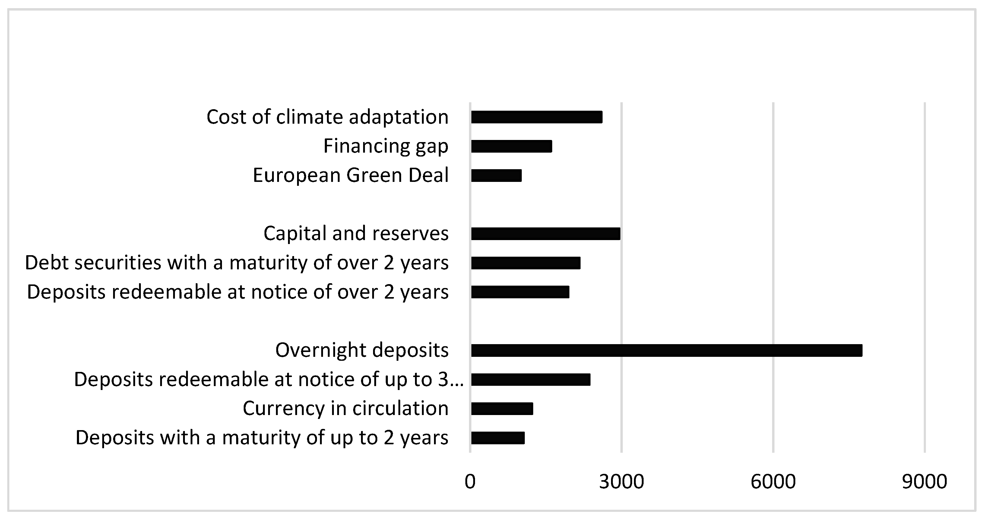
Figure 1 plots the estimated cost of climate adaptation in the European Union, together with the value of the components of monetary aggregates and long-term liabilities in the Eurozone. The figure shows that the cost of achieving the EU’s climate and energy targets exceeds the value of debt securities of a maturity of over two years, the value of deposits redeemable with a notice of up to three months, and the value of deposits with an agreed maturity of up to two years. The financing gap (calculated as the difference between the European Green Deal and the global cost of reaching the climate and energy targets), in turn, exceeds the value of currency in circulation as well as the value of short-term deposits (maturity of up to two years). These figures show that rising to the sustainability challenge will involve a disruption of the structure and the volume of assets and liabilities in the European financial system. One should also note that European budget estimates of the costs of climate adaptation are very likely to be undervalued. They do not consider, for instance, the investment needs for climate adaptation or for other major environmental challenges, such as biodiversity. They also exclude the public investment needed to address the social costs of the transition and the costs of inaction [20].
In the current context, bridging the SDG financing gap appears to involve difficult policy trade-offs. The main financing arm of the EGD is indeed the EU budget, which relies mainly on VAT and GNI-based national contributions, and its modification entails distributional consequences. For instance, the introduction of levies on household electricity and fuel consumption to fund increased contributions to the EU’s budget disproportionately affects poor households and might thus lead to an increase in inequality [21,22]. Another option might be to reallocate the existing budget across policy priorities. Indeed, the European Green Deal will mobilize 25% of the EU’s budget [20]. This, however, also entails significant distributional consequences across sectors and economies, as evidenced by ongoing discussions around the future of the Common Agricultural Policy. Finally, the climate strategy may have hidden costs and contradict other SDGs and economic convergence in the EU. For instance, according to the Polish trade union Solidarnosc, about 800,000 jobs in the coal industry are under threat because of the new European energy policies. Eastern European economies might be hurt disproportionately, given their dependency on those industries.
In this context, a contradiction appears to emerge between the legitimacy of economic policy and the imperative of funding initiatives to achieve climate goals. This contradiction may prove destabilizing both at the European level and at the national level—as demonstrated by the 2016 Brexit campaign (which promised to return the UK’s net contribution to the EU’s budget to the taxpayer) and the gilets jaunes movement in France (which started out as a protest against an ecological tax on diesel).
Research is therefore needed in order carve out new mechanisms in order to upscale SDG-related financial flows in response to sustainability demands, in a manner that is consistent with the prevailing set of political and financial constraints prevailing in the EU. In what follows, we use a history of economic thought perspective to show that the loanable fund theory (hereafter LFT)—which has come to underlie academic and policy discourse in finance—is a powerful hindrance to the adoption of SDG financing strategies by virtue of the representation that it generates. We will demonstrate that the aforementioned policy trade-offs disappear when one adopts the more realistic endogenous money theory. This allows us to identify financing pathways to achieve SDG targets in a timely manner.

3. The Loanable Fund Fallacy

3.1. The Premises of the Theory

The central tenet of the loanable fund theory (LFT) is that investment levels are constrained by the size of a preliminary pool of savings. The intellectual origins of the LFT can be traced as far back as Aristotle, J. B. Say, D. Ricardo, J. S. Mill, and most decisively Walras ’ (1874) notion of “échange d’épargne contre capitaux neufs”.
The logic of the LFT is very intuitive. Given that savings are a withdrawal from the income stream, while investment is an injection, it seems only reasonable to suppose that at the macro-economic level, savings supply the funds required for investment [23]. This idea is also confirmed by the facts of individual experience. At an analytical level however, the LFT relies on a set of specific hypotheses and adjustment mechanisms.
Regarding hypotheses, the LFT views the financial system as a market where savings are exchanged for new capital assets. Money is a veil (a numéraire) on real market exchanges, and the underlying stock of money is exogenous (i.e., provided by the Central Bank). In this representation, money is neutral: the equilibrium in the money market (and, by extension, in financial markets) merely reflects the real market equilibrium (and not the other way around). This entails a conception of financial institutions (pension, insurance and wealth funds, commercial banks, development banks, crowdfunding, venture capital, etc.) as mere intermediaries, transforming money capital into fixed assets seeking a return.
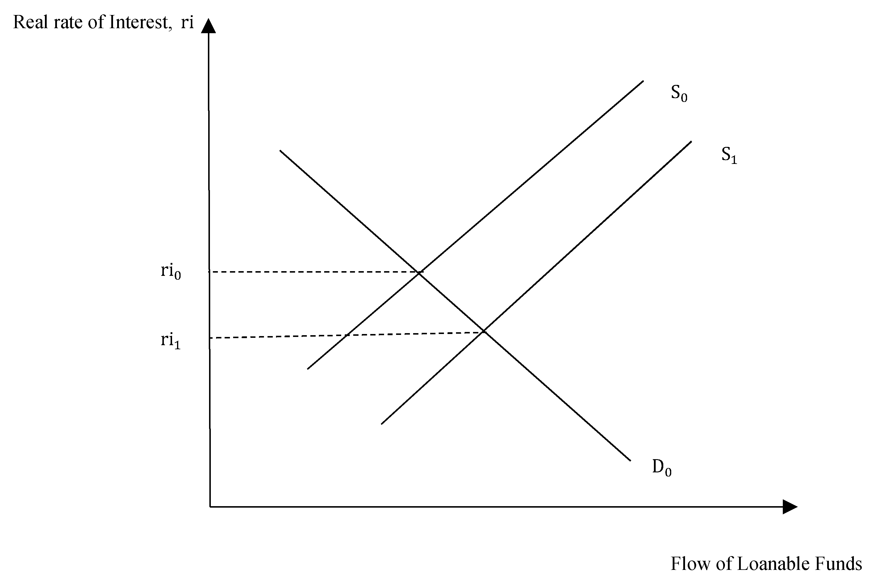
The logical consistency of the LFT rests on a classical market-based adjustment mechanism in which the interest rate—which is akin to the price of financial resources—adjusts in order to bring savings into equality with the demand for investment. In this context, any shift in the demand curve for capital or the curve relating savings to interest rate will determine the new rate of interest and a new loanable funds market equilibrium, corresponding to the intersection of the new positions of these curves. This can be illustrated with the following diagram (Figure 2):
If, for example, savings increase, the supply of loanable funds increases as the S curve shifts to the right from S 0 to S 1 . Assuming that the number of profitable projects remains unchanged, this leads to an excess supply of loanable funds. The interest rate then drops from ri 2 to ri 1 , which brings out new profitable investment projects and brings the fund market back into equilibrium. Unless thwarted by rigidities, the funds market equilibrium is characterized by “such a rate of interest that savings flow into the market at precisely the same time-rate or speed as they flow into investment producing the same net rate of return as that which is paid savers for their use” [24].
The core idea of the LFT is that “savings cause investment.” This idea is highly intuitive, and many observers adhere to it by default as it corresponds to the constraints governing individual budget, spending and debt.
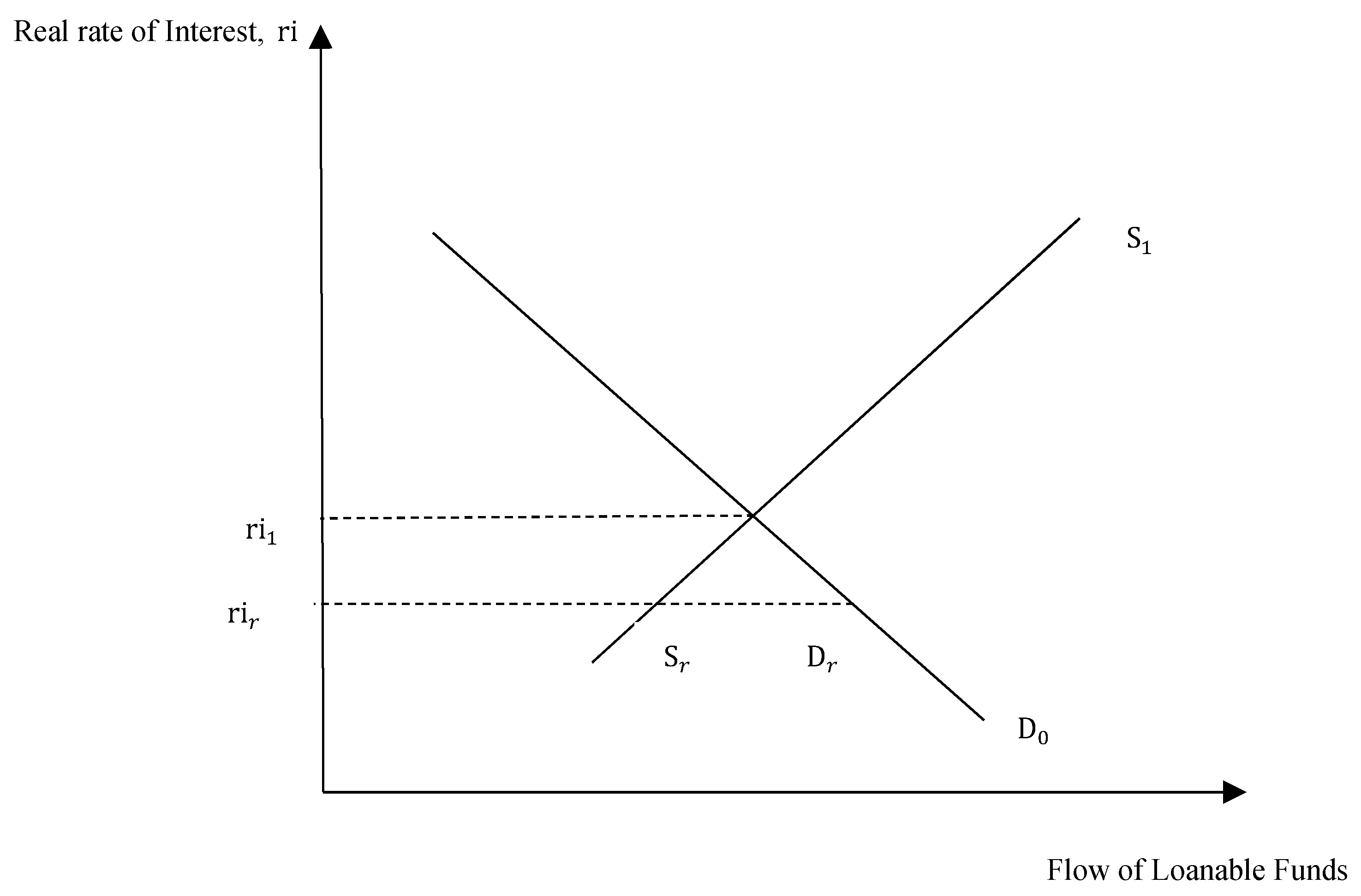
The policy implications of the LFT are far-reaching. Its key corollary is the primacy of savings: one implication of Figure 2 is that increasing corporate profits and capital income will increase the pool of savings. This, in turn, will decrease the cost of borrowed funds, and ultimately stimulate investment by increasing the marginal return on capital. Another policy corollary is the ineffectiveness of financial repression policies [25]. As represented in Figure 3, the LFT predicts that policies seeking to control financial markets (such as ceiling on interest rates, which would fix the interest rate to rir, below its equilibrium value ri1) would entail the apparition of credit rationing (the unsatisfied component of the demand for investment being represented in Figure 3 by the gap between Dr and Sr).
Overall, the widespread acceptance of the LFT offered a powerful justification for liberalization, disintermediation and deregulation policies in the financial sector. It provided a theoretical background for policies such as the decrease of taxes on capital gains, corporate profits, high salaries, and, more generally, for the trickle-down economic strategies adopted since the 1980s in many OECD countries.

3.2. LFT and the Framing of Climate Finance Policies

As seen through the lens of the LFT, the SDG finance gap is primarily an asset allocation problem. Indeed, if one is willing to accept that legitimate (public and private) investment requires preliminary savings, then the only way to bridge the sustainable finance gap is to nudge markets to allocate a greater shares of savings funds towards a new sustainable segment of ecosystem-backed securities.
At the policy level, this involves prioritizing an increase in the volume of sustainable finance assets, as well as their appropriate branding (such as ESG, SRI, and impact investing), in order to allow them to compete for funds with standard assets. The comparative advantage of sustainable finance assets in financial markets is founded on a double promise: first, a promise to make finance flows consistent with low emission and climate-resilient development; and second, a promise of maintaining a vigil for financial efficiency (the latter being again defined with reference to the concept of asset market equilibrium). Gradually, then, the SDG finance discussion has morphed into a supply-side discussion founded on the apparatus of modern finance theory, in which an additional dimension (sustainability) is added to the array of investor decision criteria (along with price, expected rate of return, portfolio diversification, equilibrium return, risk premium) [26]. Recent papers in the field of ‘sustainable finance’ have documented deviations in the price and returns of ‘green’ financial instrument from standard financial instruments [27,28], or developed new asset pricing methods, using calculation formulas defining an ‘equilibrium value’ [29].
From an SDG financing perspective, the fundamental problem with this approach is that the characteristics of the sustainable financial assets may depart from the fundamental value of the underlying real ecosystem. The trading of ecosystem-backed securities indeed necessitates the securitization of ecosystems [30]. The latter is a process by which one assigns an economic value to the ecosystem service, establishes a fungible proxy (commodification) offering a flow of payments and a tradable right to these payments. Given the functioning of financial markets and institutions, applying financial logic to sustainability issues inevitably leads to maximizing the provision of the ecosystem services that yield the largest and most stable payments. The securitization strategy may thus come at the expense of other, un-commodified, or un-commodifiable, ecosystem flows.
More fundamentally, given the complexity of ecosystem services, the traded assets cannot adequately represent the underlying value of nature. For instance, the Clean Development Mechanism (CDM), defined in Article 12 of the Kyoto Protocol, allows an industry to implement an emission-reduction project in developing countries in exchange for saleable certified emission reduction (CER) credits, each equivalent to one ton of CO2. This strategy thus implicitly equalizes ecosystem services with monetary flows derived from the market price of CO2. However, not all emission reduction strategies will have the same ecological impact. For instance, the rainforest and primitive forests, home to biodiversity, provide many more ecosystem services than artificial monoculture forests.
Overall, climate policies framed by LFT tend to create a financial hyper-reality in which the underlying system—ecosystems—is shaped to the image of the indicators supposed to represent it [31,32,33]. For instance, the infrastructure of the carbon market is based on the notion of a “price discovery” of market participants, who determine the value of the permit to place a burden on the natural ecosystem. That price is determined by a wide variety of factors, including the overall cap (including future caps), the liquidity of the market, current price information of related commodities (e.g., energy sources), demand, and forecasting for how these prices will change in the future. More generally, the market price of any sustainable financial assets depends on its trades. These are determined by a wide variety of non-ecological, market-based trends and behaviors (such as trading strategies, exposure to systemic risk, etc.). Empirical research has indeed shown that the pricing of sustainable asset portfolios does not depart from that of other portfolios traded in the same market [34]. It follows that the price of ecosystem-backed securities has a natural tendency to depart from the fundamental value of the underlying natural asset it is supposed to represent.
Finally, the ability of the securitization policy to deliver the amount of finance at an appropriate scale and speed can be questioned. As highlighted in [35] or [6], economic and financial reality is a non-ergodic and open system. The aggregate response of financial agents to nudges and labels is therefore hard to predict, given the complexity of the financial system, the emerging macroeconomic dynamics, and the resulting change in opportunities for banks and financial operators competing for profits in a globalized and technological environment.
Overall, the ecosystem-backed securitization of the environment strategy is not up to the task of providing timely and adequate financing to the SDG agenda. We contend that these problems are not a matter of labelling, incentives or calibration (i.e., what we may call “puzzle-solving” issues [36] Rather, they are the manifestation of the tacit prevalence of the LFT as the main underlying discourse in academic and policy spheres.

3.3. The LFT as a “Nonsense Theory”

Ironically, the LFT has been the object of much controversy in the history of economic thought. It was first criticized by authors such as Patinkin, Wicksell, and ultimately crumbled some 90 years ago under the attacks of John Maynard Keynes. Keynes, who unambiguously labelled the LFT a “nonsense theory” [37] (p. 155), underlined two major logical flaws of this theory.
Keynes began by acknowledging that the LFT had it right in equalizing savings with investment. Defining income (Y) as the sum of consumption (C) and investment (I) (Y = C + I), and savings (S) as the difference between income (Y) and consumption (C) indeed yields the following accounting equations:
Y = C+I
S = Y−C
S = I
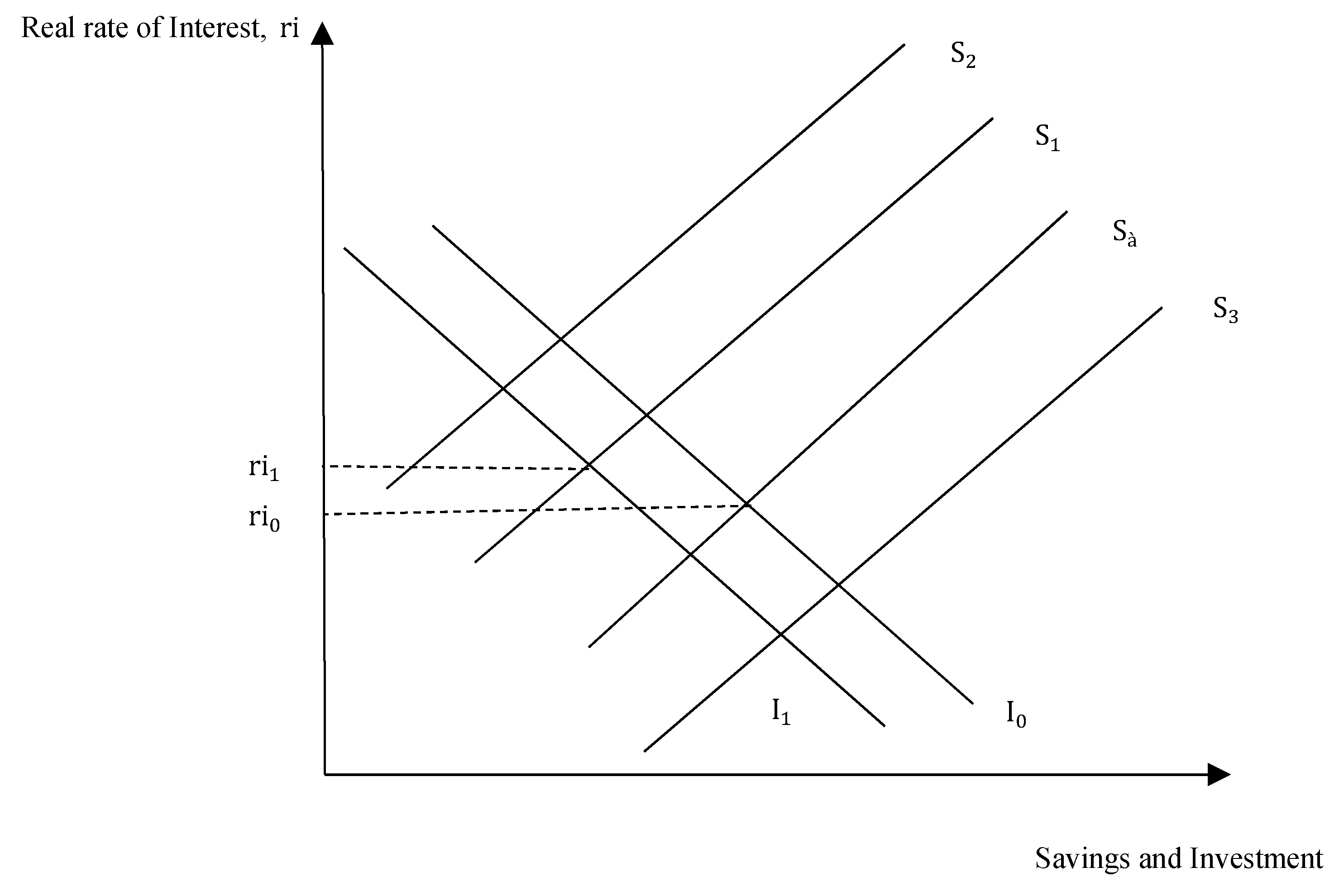
The fundamental mistake of the LFT, however, is to take Equation (3) in isolation and to infer that savings cause investment (through an adjustment of the interest rate). While this is certainly true at the individual level (one can freely decide to increase one’s savings, and thereby increase one’s financial wealth and investment capacity), at the macroeconomic level, however, savings and investment are codetermined through their relationship with income (Equations (1) and (2). This renders the LFT’s core adjustment mechanism inoperative: as shown in Figure 2, a shift of the investment curve from I0 to I1, which affects income (Equation (1)), could then trigger several possible movements of the savings curves S1, S2 or S3 (Equation (2)), leading to indeterminacy regarding the future level of interest rates. In other words, the loanable fund model fails due to the endogeneity of income.
The only way to rescue the LFT, Keynes argued, would be to assume constant income. Given Equation (1), this would require us to assume that the movements of the savings and investment curves balance each other out perfectly, so that, for instance, a given drop in consumption (i.e., an increase in savings) would be perfectly offset by a corresponding increase in investment. Nevertheless, such perfectly balanced movements would leave the equilibrium interest rate permanently unchanged in Figure 1—making, again, the LFT collapse.
The second shortcoming of the LFT identified by Keynes has to do with the determination of interest rates. The LFT indeed assumes that the savings decision is a one-step decision based on the time-preference of agents. In reality, however, savings is always (at least) a two-step decision: once the decision on how much to save out of her current income has been made, one needs to decide on what form to hold one’s savings. The most basic portfolio decision consists in determining what proportion of one’s savings will be held as money (which is liquid but does not bear interest) as opposed to other less liquid but interest-bearing assets (such as bonds or stocks). Given this fact, Keynes argued, the interest rate cannot be determined as the price “which brings into equilibrium the demand for resources to invest with the readiness to abstain from present consumption” but rather, as the price which “equilibrates the desire to hold wealth in the form of cash, with the available quantity of cash” [37] (p. 144). It follows that the savings and investment curves shown in Figure 1 do not determine the level of the interest rate. Rather, they tell us what income (and therefore the aggregate volume of employment) will be, if we know, from some other source, what the interest rate is (say, for instance, ri1) (see Figure 4).
Of course, contemporary economic and financial systems are much more complex than those prevailing in Keynes’ days. Recent theories of interest rates underline a wide array of explanatory factors including bank-lending practices, the demand for money, the monetary policies of the Central Bank, prudential regulations, and the shape of the yield curve [38]. Keynes’ core message, nonetheless, remains valid: the determination of interest rates obeys economic forces more complex than the time-preference of savers and the “supply” of capital assets.).
Rejecting the LFT has far-reaching policy implications. The most fundamental one is that savings are no longer considered to be a factor which will increase investment, but, rather, as a societal scourge, which decreases income and employment. Recent econometric work validates this view by showing that the development of the financial sector is actually detrimental to economic growth, wages and investment in OECD countries, especially since the 2008 crisis [39]. Policy recommendations that follow typically include the curtailing of financial markets, the taxation of multinational corporate profits, the adoption of stricter regulation of speculative activities—including secrecy jurisdictions—or the adoption of higher marginal tax rates.
But if one is willing to accept that investment and interest cannot be solely explained by savings, then one needs to frame sustainable finance policies from a different perspective than the LFT-based issuing of ecosystem-backed securities. As we shall see in the next section, the post-Keynesian endogenous theory of money provides a more realistic theoretical account of the relationship uniting savings, investment, and the economic system, and permits to identify fresh strategies to bridge the sustainable finance gap.

4. The Post-Keynesian Endogenous Theory of Money

4.1. A Transaction Flows Matrix

Following the seminal work of Godley and Lavoie [19], we use a consistent theoretical and accounting framework to present an up-to-date explanation of the endogenous theory of money. We begin by realistically integrating the real and financial sector sides of a simplified economy using a transaction flows matrix (Table 1). Each economic transaction in the matrix is double-sided, i.e., one’s income corresponds to another’s spending, and one’s asset is always another’s liability. Changes to the stock of assets and liabilities by each sector (in columns) result from its budget constraint, and the latter depends on flows of income and spending (in rows). Changes to each sector’s stock of assets and liabilities at the end of each period appear in the shaded area of Table 1.
The coherence of the matrix, in which a (+) sign indicates a source of funds and a (-) sign indicates a use of funds, is built on double entry bookkeeping logic: each row and each column must sum to zero. At first glance, the matrix reveals that savings and investment appear, not as the determinants of the economic system, but rather as their twin determinates. For instance, positive household savings is a surplus of income over spending that materializes as assets appearing in the balance sheets of households, and as liabilities in the balance sheet of the issuing sector. Whether a given sector issues liabilities (or accumulates assets) at the end of each period, however, depends on a complex set of interrelated macroeconomic, behavioral, institutional factors, which determine the flow of transactions in a manner that is always consistent with accounting rules. The LFT conception of money as a “given stock,” which has no counterpart in the rest of the economy, hence appears meaningless.
The matrix comprises four sectors: the household sector, the production firm sector, the public sector (made of a government and its Central Bank), as well as a relatively sophisticated financial sector based on recent development in post-keynesian economics [40]. The financial sector comprises banks and a “shadow-banking sector” comprising money market mutual funds, broker-dealers and special purpose vehicles. Macroeconomic income appears as a memo, in line with Equation (1): the excess of income over consumption (i.e., savings) cannot differ from the addition to investment.
Column 1 shows the budget constraint of households. Households receive various flows of income such as wages (W), dividend payments (from equity holdings in production firms ( F D f ), banks ( F D b ), and money market mutual funds ( F D m )), and interest on their banking deposits ( r m ( 1 ) M h ( 1 ) ). They spend their income on consumption (C), interest payments on their loans ( r l ( 1 ) L h ( 1 ) ) and tax payments net of transfers ( T h ). Any surplus of income over spending adds to their stock of assets. The latter comprises cash ( H h   ), bank deposits ( M h   ), and equities, which are issued by banks ( e b p e b ), production firms ( e f p e f ) and money market mutual funds ( e m f p e m f ). Any excessive spending relative to income implies a decrease in assets or an increase in household debt ( L h   ).
Column 2 shows the receipts and outlays of production firms in their current account. Firms receive payment flows on their sales of final goods (C) and capital goods (I), pay wages (W), taxes ( T f ) and interest on their bank loans ( r l ( 1 ) L f ( 1 ) ). Column 3 shows that firms’ capital expenditures are financed via retained earnings ( F U f ), new loans ( L h   ) or equity issues ( e f p e f ).
Columns 4 to 8 describe a financial sector comprising banks and a simplified shadow banking system with money market mutual funds, broker-dealers and special purpose vehicles.
Columns 4 and 5 show the current account and the capital account of banks. Banks receive interest payments on loans ( r l ( 1 ) L ( 1 ) ), on their T-bill holdings ( r b ( 1 ) B b ( 1 ) ), and pay interest on their clients’ deposits ( r m ( 1 ) M ( 1 ) ). The difference constitutes their profit ( F b ), which is split between dividend payments ( F D b ) and retained earnings ( F U b ). These retained earnings, along with the new deposits ( M ) and equity issues ( e b p e b ), appear on the liability side of banks’ balance sheets. They are the counterpart to the assets owned by banks, which include granted loans ( L ), high-powered money (cash and reserves) ( H ) and T-bills ( B b ).
Column 6 describes the money market mutual funds (MMMFs). MMMFs issue equities ( e m f p e m f ) in exchange for banking deposits ( M h   ). They also hold Treasury bills ( B m   ), which they purchase from broker-dealers in reverse repo operations. They distribute all their profits to households ( F D m ).
Columns 7 and 8 describe broker-dealer (BD) entities and special purpose vehicles (SPVs), which are both subsidiaries of commercial banks. Broker-dealers hold T-bills ( B m   ), which they sell to MMMFs in repo operations in exchange for banking deposits ( M h   ), and hold MBS shares issued by special purpose vehicles ( e s p v p s p v )   . Special purpose vehicles issue mortgage-backed securities (MBSs) ( e s p v p s p v ) and use the proceeds to purchase loans from the banks ( e s p v p s p v )   . Profits of broker-dealers and SPVs ( F b d and F s p v ) are distributed back to the banking sector.
Column 9 describes the budget constraint of the government. It shows that any investment expenditure ( I g ) that is not financed by taxes ( T b ) (or by Central Bank dividends F c b ) must be financed by an issue of T-bills ( B ). Following Godley and Lavoie [19], in our matrix the interest on T-bills paid by the government to the Central Bank is returned to the government, so that net interest disbursement is: r b ( 1 ) B b ( 1 ) r m ( 1 ) B m ( 1 ) + r b ( 1 ) B c b ( 1 ) .
Columns 10 and 11 represent the current account and the capital account of the Central Bank. The Central Bank owns T-bills ( B c b   ) and its main liability is the high-powered money (cash and reserve currency) that it issues ( H ). Any addition to the bond portfolio of the Central Bank must be accompanied by an increase in the amount of high-powered money. Central Bank profits (equal to the T-bill rate) are transferred to the government ( F c b ).

4.2. Credit, Finance and Savings: the Endogenous Money Perspective

The transactions flow matrix shown in Table 1 is a useful device with which to analyze the financing of the economy from an endogenous money perspective. This starts by acknowledging that private banks do not lend preexisting funds, but instead create new credit money every time they grant a loan [15]. There are, of course limits to the power of banks to create money. Banks must meet profitability constraints in order to remain competitive and must ensure that the firm has a capacity to repay. They must also abide by prudential regulations, in particular capital requirements. Finally, banks must be able to acquire reserves at a low cost if the firm wants to spend its deposits. Therefore, even though banks can create unlimited amounts of deposits, they have no incentive to do so because it may expose them to both insolvency and illiquidity risks. Examining the actual functioning of a banking system shows, nonetheless, that the causality relationship does not run from savings to investment (as indicated by the LFT) but, in fact, in the opposite direction.
We may illustrate this through the simplest case, where a bank extends a loan to a firm that wishes to extend its production capacity. Table 2 accordingly focuses on the relevant entries in the transaction matrix. It shows that credit creation entails four balance sheet entries: a new deposit enters the bank’s balance sheet on the liability side and the borrower’s balance sheet as an asset; and a new loan, which enters the bank’s balance sheet as an asset and the borrower’s balance sheet as a liability As opposed to popular belief, there is no ex-ante intermediation when a bank grants a loan, since both sides of the balance sheet (the loan/the deposit) involve the same client [41].
As soon as the firm undertakes investment by spending its new deposits on wages (W), macroeconomic income increases (in line with Equation (1)). New deposits are transferred to the bank account of the households providing the goods and services to the firm. These deposits are income not spent—which means, at an accounting level, that savings go up. Of course, the loan’s counterpart is the saver’s deposit, but there should be no confusion regarding causality: the loan is financed by an ex-nihilo money creation [40] The bank can be thought of as an “ex-post” intermediary [38,42].
As households provide labor in exchange for the salaries, firms accumulate inventories, which appear on their capital account (I) as the ex-post counterpart of the bank loan. Finally, households spend a part of their income on consumption (C). This allows firms to retrieve their money balances and to repay the initial bank loan. At this point, the credit money, which allowed production in the first place, is destroyed, as the bank’s balance sheet shrinks on both sides. This mechanism is fully consistent with Equations (2) and (3): following an increase in investment, income will increase to a level that makes the change in savings equal to the change in investment.
The conclusions of the LFT are therefore turned upside down. At the macroeconomic level, net accumulation of savings necessitates a preliminary increase in debt-financed investment (and not the other way around).
Denis [43] offers an even simpler demonstration. Letting W represent the wage bill, S represents household savings, and I represents firms’ net investment in a given year, the economy’s sale of final goods is equal to household consumption (W-S) plus net investment (I). Firm profits π are, in turn, equal to the difference between sales (W-S+I) and the wage bill W, i.e., π =I-S. Profits thus correspond to the share of firms’ net investment which is not financed by savings.
In the post-Keynesian view, finance and savings are therefore two very different things. Finance is a flow of credit determined on the basis of entrepreneurial expectations, while savings are a residual stock caused in the first place by macroeconomic dynamics. This has practical implications exactly opposed to those implied by the LFT. In particular, increase in savings by the household sector (a “thrift campaign”) does not result in increased investment. Instead, it implies a direct loss of income for production firms (as consumption spending (C) decreases). This loss is unlikely to trigger new investment plans. It is more likely to lead to the formation of pessimistic entrepreneurial expectations, which reduces the investment rate and, ultimately, the accumulation of financial wealth —i.e., savings—at the next period.
These basic observations are by no means new, and have been known at least since the work of Keynes (1936). The fact that they seem to have been forgotten by most financial economists—outside of the post-Keynesian tradition—has led certain authors to conclude that we live in a “dark age of macroeconomics” [44].

4.3. Incorporating “Shadow Banking” into the Analysis

The development of the so-called “shadow banking system” (also called “non-bank finance” or “market based” finance) is an important feature of the modern economy (Lagoarde-Segot, 2015). In the endogenous money perspective, shadow banking does not provide additional financing to the economy, but adds layers of debts within the financial sector, based on a pre-existing stock of banking deposits. As indicated in [40] (p. 17): “The raw materials used by the shadow banking system to produce securities are created by traditional banks, so the former cannot expand if the latter does not grow in the first place.”
Assume for instance that households decide to rebalance their portfolio and buy shares issued by the money market mutual fund (MMMF). A fraction of banking deposits M h A S S E T (which were created, in the first place, through production credit, as in Table 2), are then transferred from the household’s account to the MMMF’s account in exchange for shares ( e m f p e m f   ). These deposits still appear on the liability side of the banking sector’s balance sheet. This situation is shown in Table 3 below.
The MMMF then enters into a reverse repurchase agreement with a broker-dealer. The broker-dealer sells a T-bill to the MMMF ( B m A ), agreeing to repurchase it at a future date. As shown in Table 4, the banking deposits now appear on the asset side of the broker-dealer’s balance sheet.
This situation does not last very long, as the broker-dealer uses these acquired deposits to purchase MBSs issued by a special purpose vehicle (Table 5).
The SPV, in turn, uses the deposits to buy packages of loans from the commercial bank. As a result, the bank moves the loans off its balance sheet, which destroys a corresponding amount of credit money (Table 6).
In summary, the shadow banking system entails the issuing of a chain of liabilities (ownership rights and a portfolio of pre-existing loans (MBSs)) against an initial flow of banking deposits. This scheme permits banks to move loans out of their balance sheet, and gives them incentive to finance riskier projects. In the endogenous money perspective, the shadow banking system adds layering, complexity, and fragility to the financial system without altering the fundamental macroeconomic causality running from credit to deposits and from investment to savings. Quoting Keynes, “the investment market can become congested through a shortage of cash. It can never become congested through a shortage of savings” [37] (p. 222). The next section attempts to carve out policy responses to the sustainable finance gap using endogenous money theory as a conceptual framework.
5. In search of New Financing Pathways

5.1. Sovereign Green Bond (SGB) Issues

5.1.1. The Case for SGB Issues

Sovereign green bond (SGB) issues would probably be the most direct way to make available the money needed to tackle the climate crisis, whilst avoiding pitfalls related to the securitization of ecosystems. The direct counterpart of SGBs would be vigorous action geared towards energy transition (such as renovation and energy efficient buildings, renewable energy generation and transmission, and low-carbon transportation, to name a few) or climate resilience investment (to counteract flooding, heatwaves, drought, cyclones, wildfires, and other extreme climate events).
SGBs would permit to bridge the SDG finance gap without raising new taxes, and hence avoid the distributional trade-offs discussed in Section 2 of this paper. SGBs—a form of T-bills—are the cornerstone of financial markets. Financial theory refers to T-bills as the “risk-free asset” because illiquidity and insolvency risks are nil if the government borrows in a sovereign currency [44,45]. Security-pricing models (such as the CAPM) indeed proceed by adding an asset-specific mark-up (the risk-premium) to the T-bill rate of return in order to determine equilibrium investment return. SGBs would therefore represent a new category of risk-free assets that could be purchased by banks and pension funds that have strong regulatory incentives to do so (the ponderation is 0% under pillar I of Basel’s solvability ratios).
One should note that sovereign currency issuers have often issued T-bills in order to tackle tough circumstances. One classical historical example is the financing of the US Arsenal for Democracy during WWII. In contrast with the European belligerents’ WWI finance policies—which relied mostly on taxes and foreign borrowings—US involvement in WWII was, to a very large extent, financed through close collaboration between the US Treasury and the Federal Reserve. The US Treasury issued as many T-bills as was necessary to finance the war-related purchases. In turn, the Federal Reserve supplied banks with adequate reserves to purchase these T-bills, of which it directly purchased large amounts itself. This kept the cost of deficit financing as low as possible, while pegging the interest rate on short-term and long-term Treasury bills at 0.375% and 2.5%, respectively [46]. These unusual policies enabled a rapid and automatic increase in American military expenditure, which rose from a few hundred million dollars a year before the war to USD 85 billion in 1943 and USD 91 billion in 1944.
Beyond financial issues, SGBs would involve a strong policy stance at the European level. As discussed in [3], state funding has often provided the initial push, early state, high-risk funding and institutional environment that were behind most technological revolutions, in the pharmaceutical, communication and IT sectors, or the green energy sector. In the current climate crisis, the “entrepreneurial courage of the State” may thus contribute to a structural transformation of economies towards a circular model [3].
One legitimate area of concern, however, is the applicability of this strategy, given the prevailing institutional rules in the Eurozone. Indeed, the Stability and Growth Pact places a ceiling of 3% for budget deficit and 60% for public debt (relative to GDP). One should note, however, that existing treaties provide a legal basis for sustainability targeted sovereign bond issues. Indeed, Article 119 of the Treatise on the Functioning of the European Union stipulates that the activities of the Member States shall include the adoption of an economic policy for the purposes set out in Article 3 of the Treaty on the European Union. This article, in turn, establishes sustainable development as a guiding principle of member countries. There is hence a legal case for Eurozone governments to subtract sovereign green bond issues from the calculation of deficit ratios [47]. More fundamentally, the Stability and Growth Pact can be changed by decision of the European Council. It was indeed amended in 2005 to add exemptions to the deficit rule (taking into account behavior of the cyclically adjusted budget, the level of debt, the duration of the slow growth period, and the possibility that the deficit is related to productivity-enhancing procedures).

5.1.2. SGB Issues in the Eurozone

In the Eurozone—as opposed to other monetary systems such as the US, Sweden, the UK or Japan—the Central Bank refrains, except under exceptional circumstances (“outright monetary transactions”), to directly purchase Treasury securities from the government (as per Article 123 of the Lisbon Treaty). In what follows, we will therefore examine the impact of the sovereign green bond issue on the various parties involved in this particular institutional setting. We will use the analytical framework provided in [44], and we will assume that the government is spending in the private sector to undertake its climate policy (note, however, that the results would be unchanged were spending made in the public sector).
One should nonetheless bear in mind that institutional settings regarding the issuing of T bonds change over time, as governments have the power to change the rules that they write and self-impose regarding the creation of credit money. As the paper goes to print, on March 18th, 2020 the European Central Bank’s Governing Council announced that it would do “everything necessary within its mandate,” “as much as necessary and for as long as needed” to counter the economic risk of the COVID-19 pandemic. Its first decision was to launch an asset purchase program of private and public sector securities with an initial envelope of EUR 750 billion.
The SGB process begins when the government’s Department of Finance and Department for Sustainability identify and budget a set of priority investments that would be required to tackle climate crisis. Ideally, external stakeholders (such as banks, investors, insurance companies) would be involved early in the structuring and pricing process of the SGB through appropriate platforms, such as a Public–Private Green Bond Advisory Council. The Treasury is then in charge of issuing a fresh green bond in order to finance this climate strategy.
In the first step, a bank borrows reserves from the Central Bank (against collateral) in order to purchase the SGB. As shown in Table 7, this operation results in four accounting entries: the new loan enters in the asset side of the Central Bank’s balance sheet, and on the liability side of the bank’s balance sheet; the new reserves enter in the asset side of the bank’s balance sheet and on the liability side of the Central Bank’s balance sheet. At this stage, the balance sheets of the Treasury and the private sector are unchanged.
Banks then transfer the reserves to the account of the Treasury at the Central Bank in order to purchase the new SGB. In this step, the balance sheet of the Central Bank is unchanged; however, the reserves now belong to the Treasury. In the Treasury’s balance sheet, this new asset is matched by a new liability, which itself appears as an asset in the bank’s balance sheet. This is shown in Table 8 below.
The government’s Department for Sustainability now spends the proceeds of the SGB issue to implement its climate policy. As shown in Table 9, new banking deposits thus appear on the asset side of the production firm’s balance sheet, and on the liability side of the bank’s balance sheet. A corresponding increase in reserves, drawn from the Treasury’s account at the Central Bank, also enters the asset side of bank’s balance sheet.
The bank is now in a position to repay its reserves loan to the Central Bank. The final positions of the balance sheets are shown in Table 10:
As can be seen, this policy leads to a net increase in private sector wealth. Indeed, the private sector now holds new banking deposits, and banks hold a new interest-bearing SGB. In the process, real resources (labor, technologies) have been allocated to the pursuit of SDGs.

5.2. Greening Macro-Prudential Policy

Endogenous money theory also provides insight into the mechanisms by which credit creation and banking behavior can be aligned with SDG priorities. This, however, requires that a ‘sustainability taxonomy’ of assets has been established. In the words of the European High-Level Expert Group on Sustainable Finance, (2018) such a taxonomy should allow us to identify “under which conditions or criteria any given investment or financial product will contribute to the EU’s sustainability objectives” [4] (p. 15).
Assuming such a taxonomy, Table 11 now divides the production sector into the “non-SDG sector” and the “SDG sector.” It also divides bank loans—and deposits—into loans made to the non-SDG sector ( L f   ) and to the SDG sector ( L f , s d g   ). Our zero-sum rule ensures that the flow of lending is equal to loan assets held by the banking sector ( L f   + L f , s d g   = L ).
In this Table, banks now also hold both regular T-bills and SGBs in their portfolio of assets. Of course, banks hold many other assets in their balance sheets but adding them into the matrix would add unnecessary complexity. In what follows, we use this simple setting to discuss a set of prudential policies that would entice banks to issue a particular portion of their credit to specific sectors of the economy, and to rebalance their portfolio of assets towards SGBs.
In particular, Table 12 shows two indicators that the European Central Bank could use as part of its prudential policy. The first indicator tracks credit to the SDG sector as a proportion of total credit. Reaching the target value of this indicator for a given year (so that, for instance,   L f , s d g   L   = x % ) would imply that x% of the newly created credit money ( M h   ) circulating in the economy was issued in response to SDG investment demands that year. The second indicator measures the share of SDG-contributing assets in banks’ balance sheets. Reaching the target value of this indicator for a given year would keep the financing costs low for SDG-related asset issuers (in particular SGBs) by maintaining adequate demand. Increases in SDG sector asset holdings will also increase the financing costs for non-SDG sector assets—and provide incentives to align production structures in the economy with sustainability objectives.
These policies entail a redefinition of the Eurosystem’s mandate. This redefinition, however, appears aligned with the Treaty on the European Union. Article 3 of the 1993 Maastricht Treaty on the European Union states: “The Union shall establish an internal market. It shall work for the sustainable development of Europe based on balanced economic growth and price stability, a highly competitive social market economy, aiming at full employment and social progress, and a high level of protection and improvement of the quality of the environment.”).
It may also contribute to the European Central Bank’s core objective of price stabilization by diminishing the impact of climate change on the European economy. It is indeed recognized that physical risks will turn into financial risks and affect the prices of assets and macroeconomic dynamics [48]. Finally, one should also note that the Eurosystem has been able to show remarkable flexibility and resilience when faced with a crisis context. The sovereign debt crisis of 2010–2013 led to vigorous responses, such as the interdiction of naked CDS operations and strict supervision of short selling in November 2011, and the announcement of “outright monetary transactions” in August 2012. Similarly, on 18 March 2020 the European Central Bank made the following announcement in response to the outbreak and escalating diffusion of COVID-19: “To the extent that some self-imposed limits might hamper action that the ECB is required to take in order to fulfil its mandate, the Governing Council will consider revising them to the extent necessary to make its action proportionate to the risks that we face.”
A redefinition of the Eurosystem’s mandate to achieve EDG objectives therefore appears within reach. In a letter to the European Parliament, former ECB President Mario Draghi announced that the Eurosystem “should support the sustainable development of Europe,” while underlining that “it falls to the political authorities to define and decide on the appropriate measures to achieve the objectives of the Paris agreement” [49].
In what follows, we discuss policy tools that would upscale the banking sector’s contribution to the SDG agenda. These policies include, for instance, the modification of the ECB’s collateral framework, amendments to capital adequacy ratios, the development of a lending certificates trading platform, and the introduction of rediscounting policies for SDG loans.

5.2.1. Modifying the ECB Collateral Framework

By law, Eurozone banks need to hold reserve deposits with the European Central Bank of 1% of the value of their deposits with a maturity of up to two years. The ECB, in turn, has to provide reserve on demand at its base interest rate, up to the value of the collateral pledged by the bank requesting reserves. Reserves therefore do not, in any way, constrain lending in the economy [15,44,45]. To determine the bank’s borrowing capacity, the European Central Bank nonetheless applies a “haircut” to the value of the collateral supplied by a bank. For instance, if the bank provides a collateral of a value of X and the haircut rate is 5%; the ECB will lend (X/1 + 5%) euros in reserves. This loan, backed up by collateral, is the Central Bank’s asset, as shown in Table 13.
The ECB currently determines the haircut category of an asset by combining asset type and issuer group criteria [50]. Supervisory authorities regularly review these haircut categories from a risk perspective. Adjusting the haircut applied to different assets and issuers would be an effective way to maintain banks’ appetites for SDG assets (such as SGBs).
The ECB may decide, for instance, to decrease its haircut for SDG assets, and increase it for “brown assets.” This policy, which would amount to a modification of the asset-type classification system, would sustain the demand for SGBs in financial markets. The Central Bank could also modify its haircut rate for banks that meet or fail to meet the indicators in Table 9. Banks that extend excessive loans (or hold assets) to the non-SDG sector would receive a higher haircut. This would amount to a modification of the issuer-group classification system.
One should note that there are several historical examples of the Central Bank modifying its collateral frameworks in order to reach certain socioeconomic objectives. For instance, the Banque de France’s decision to accept railway equities and bonds as collaterals in the late nineteenth century provided significant support to the development of the railway industry in France: “After the coup which led to the ‘Second Empire’, the government asked the Banque de France to accept the railway companies’ bonds and equities as collateral in discount operations and also for loans to any private person. It also asked the Banque de France to lend money to the railway companies ahead of new issuances and to place such issuances in the market. These measures helped the railway companies in financing their activities, at a time when they have faced constraints and had been prompted to merge among themselves by the government.” [51] (p. 907). More recently, the European Central Bank eased the Eurosystem’s collateral standards by modifying its issuer group classification system; as part of its 2020 Pandemic Emergency Repurchase Program. The policy consisted in expanding the scope of Additional Credit Claims (ACC) to include claims related to the financing of the corporate sector.

5.2.2. SDG Lending Certificates

The creation of a market for SDG lending certificates, in the spirit of the Indian Priority Sector Lending Certificates (PSLCs) is another way to incentivize banks to adopt a pro-SDG strategy. In India, the Central Bank establishes priority sector lending targets for the banking sector (such as agriculture, education, or small and medium-sized enterprises (SMEs)). At the end of each year, each bank reports its SDG lending achievement as the sum outstanding of its priority sector loans as a proportion of its new credit ( L f , s d g   L   ). Some banks may fail to lend to the priority sectors (i.e.,   L f , s d g   L < x %   ) while other banks lend more than their specified target sectors (i.e.,   L f , s d g   L > x %   ). In order to achieve targeted lending to priority sectors, banks can sell and purchase Priority Sector Lending Certificates (PSLCs) through a trading platform managed by the Central Bank. The banks with surplus sell fulfillment of priority sector obligation, and the buyer banks buy the obligation with no transfer of risk or loan assets. The fee is determined through market-based mechanism. This strategy incentivizes surplus banks to sell their excess achievement and encourages banks to lend more to the SDG sector.

5.2.3. Amending Capital Requirements

Under Basel III, the minimum capital adequacy ratio that banks must maintain (including the capital conservation buffer) is 10.5%. The capital adequacy ratio measures a bank’s capital in relation to its risk-weighted assets. Changing risk weights to entice banks to hold greener assets is an option currently championed by several banks. However, as pointed out by Finance Watch [52], sector-specific risk-weight adjustments as high as 25% have been experienced in the EU for SME lending, with little or no impact on the volume of loans [53]. Generating sufficient volume of credit would thus necessitate large changes to risk weights and may come at the cost of higher systemic risk (allowing banks to increase their leverage). Another option would be to raise risk weights for brown assets. This would strengthen financial stability while discouraging lending for fossil fuel activities.

5.2.4. Rediscounting Policies

Another policy option, which the ECB could use to incentivize banks, would be to rediscount SDG-sector loans. Under such policies, banks directly obtain loans and advances from the Central Bank, using their loans as collaterals. The impact on the balance sheet of the bank and the ECB would be similar to the one showed in Table 10 (with the difference that the amount obtained would cover the value of the loan, rather than reserve requirements). Rediscounting has fallen out of favor in most OECD countries, but was mainstream until the 1990s, especially in developing countries. In a 1985 report on lending to small enterprises, the World Bank stated that “the most successful arrangement in inducing commercial banks to become intermediaries is that of having an agency to rediscount the loans made by lending institutions” [54] (p. 22). Rediscounting was also used successfully in France where, in the aftermath of WWII, the rediscounting of loans by the Banque de France was allowed for a maturity of up to five years. These operations permitted to raise FRF 50 billion in July 1947 and to finance large-scale investment programs in nationalized utilities (coal and electricity) and automobile enterprises [55]. Similarly, during WWII, where the US government established a program of guaranteed loans to speed up industrial expansion in the war, loans under USD 100,000 (i.e., more than half of all loans) were directly handled on the spot by reserve banks and branches. Finally, many Central Banks in developing countries (e.g., Philippines, Nigeria, or India) currently use rediscounting policies to provide sufficient financing to priority sectors. More recently, the European Green Deal platform championed this approach by calling for the European Investment Bank to issue long-term green bonds, which would then be repurchased by the European Central Bank as part of its asset-purchasing program [17]. Such rediscounting schemes are also very likely to be used to counteract the economic consequences of COVID-19 in Europe.

6. Conclusions

This paper sought to inform action needed by policy makers, financial actors, and public and private investors in order to upscale SDG financial flows in response to sustainability demands. We first documented the magnitude of the SDG finance gap in the EU and discussed some of the trade-offs faced by European policy makers. We then argued that such trade-offs are largely the result of the hegemony of the loanable fund theory (LFT), which has come to dominate academic and policy discourse in the past decades. Using a history of economic thought perspective, we highlighted the logical flaws of the LFT and called for its replacement by the more realistic endogenous money theory put forth by post-Keynesian authors. We discussed recent developments in the endogenous money theory using a consistent social accounting matrix transaction flows matrix, in the spirit of Godley and Lavoie [19]. Finally, we used it as a grid to introduce a set of simple financial mechanisms, which would allow the quick release of the amount of finance required for SDG-related transformative investments. These mechanisms—which are by no means exhaustive—include the issuing of sovereign green bonds, and the greening of money creation by banks through a modification of the European Central Bank’s collateral framework, changes in capital adequacy ratios, SDG lending certificates and rediscounting policies.
Designing successful policy strategies will require feedback from policy officials, financial industry actors, and citizens, and will also require us to pay attention to specific political, economic, and institutional contexts. Successful policy deployment will also have to match monetary resources with real, tangible objectives, and ensure maximum transparency and accountability. However, the message is clear: given the challenges of our circumstances, a paradigm change is necessary. Endogenous money theory offers vast avenues for conceptualizing and implementing the policies needed to tackle the challenges we are facing. Future research could contribute to this discussion, for instance, by building upon the balance sheet approach used in this paper to simulate the impact of such policies through stock-flow consistent models.
In the end, our paper proposes a rather positive outlook on the climate finance debate. Our central thesis is that the SDG financing dilemmas are primarily the result of an optical illusion induced by the deforming lens of the loanable fund theory. It follows that the relevant question is not whether the EU—or the world—can finance the EGD agenda, but whether sufficient real resources—labor, equipment, and technology—will be available to tackle the climate crisis and achieve SDGs.

Funding

This research received no external funding.

Acknowledgments

I would like to thank three anonymous referees for their useful comments and suggestions.

Conflicts of Interest

The author declares no conflict of interest.

References

  1. SDSN. Closing the SDG Budget Gap. Move Humanity; SDSN Global: New York, NY, USA, 2018. [Google Scholar]
  2. McCollum, D.; Nagai YRiahi, K.; Marangoni, G.; Calvin, K.; Pietzcker, R.; Van Vliet, J.; Van der Zwaan, B. Energy investments under climate policy: A comparison of global models. Clim. Chang. Econ. 2013, 4, 1–37. [Google Scholar] [CrossRef]
  3. Mazzucato, M. The Entrepreneurial State. Debunking Public vs. Private Sector Myths; Public Affairs: New York, NY, USA, 2015. [Google Scholar]
  4. High-Level Expert Group. Financing a Sustainable European Economy. Final Report of the High-Level Expert Group on Sustainable Finance; HLEG: Brussels, Belgium, 2018. [Google Scholar]
  5. Lagoarde-Segot, T. Diversifying financial research: From financialization to sustainability. Int. Rev. Financ. Anal. 2015, 39, 1–6. [Google Scholar] [CrossRef]
  6. Lagoarde-Segot, T. Sustainable finance. A critical realist perspective. Res. Int. Bus. Financ. 2019, 47, 1–9. [Google Scholar] [CrossRef]
  7. Lagoarde-Segot, T.; Paranque, B. Finance and sustainability: from ideology to utopia. Int. Rev. Financ. Anal. 2018, 55, 80–92. [Google Scholar] [CrossRef]
  8. Alijani, S.; Karyotis, C. Sustainability: Finance, Economy, and Society; Emerald Group Publishing: Bingley, UK, 2016. [Google Scholar]
  9. Paranque, B.; Pérez, R. Finance Reconsidered: New Perspectives for a Responsible and Sustainable Finance. Critical Studies on Corporate Responsibility, Governance and Sustainability; Emerald Group Publishing Limited: UK, 2016; Volume 10. [Google Scholar]
  10. Steffen, W.; Broadgate, W.; Deutsch, L.; Gaffney, O.; Ludwig, C. The trajectory of the Anthropocene: The Great Acceleration. Anthr. Rev. 2015, 2, 81–98. [Google Scholar] [CrossRef]
  11. Chiapello, E. The Making of Finance. Perspectives from the Social Sciences. The Work of Financialisation, Chapter 21; Chambost, I., Lenglet, M., Tadjeddine, Y., Eds.; Routledge: Oxon, UK, 2019. [Google Scholar]
  12. Chambost, I.; Lenglet, M.; Tadjeddine, Y. (Eds.) The Making of Finance: Perspectives from the Social Sciences; Routledge: Oxon, UK, 2019. [Google Scholar]
  13. Muniesa, F. The Provoked Economy. Economic Reality and the Performative Turn; Routledge: Oxon, UK, 2015. [Google Scholar]
  14. MacKenzie, D.; Millo, Y. Constructing a market, performing theory: The historical sociology of a financial derivatives exchange. Am. J. Sociol. 2003, 109, 107–145. [Google Scholar] [CrossRef] [Green Version]
  15. Bank of England. Money creation in the modern economy. Q. Bull. 2014, 1, 14–27. [Google Scholar]
  16. Dafermos, Y.; Nikolaidi, M.; Galanis, G. Climate change, financial stability and monetary policy. Ecol. Econ. 2018, 152, 219–234. [Google Scholar] [CrossRef]
  17. Green New Deal for Europe. Blueprint for Europe’s Just Transition. 2019. Available online: https://www.gndforeurope.com/10-pillars-of-the-green-new-deal-for-europe (accessed on 27 March 2020).
  18. Veblen Institute for Economic Reforms. “Drone Money” to Put Monetary Policy Back to the People; Couppey-Soubeyran, J., Carré, E., Lebrun, T., Renault, T., Eds.; Veblen Institute for Economic Reforms: Paris, France, 2020. [Google Scholar]
  19. Godley, W.; Lavoie, M. Monetary Economics. An Integrated Approach to Credit, Money, Income, Production and Wealth; Palgrave-MacMillan: London, UK, 2012. [Google Scholar]
  20. European Commission. The European Green Deal; European Commission: Brussels, Belgium, 2019. [Google Scholar]
  21. Zachmann, G.; Fredriksson, G.; Claeys, G. The Distributional Effects of Climate Policies; Blueprint 28; Bruegel: Brussels, Belgium, 2018. [Google Scholar]
  22. Hall, S.; Roelich, K.E.; Davis, M.E.; Holstenkamp, L. Finance and justice in low-carbon energy transitions. Appl. Energy 2018, 222, 772–780. [Google Scholar] [CrossRef]
  23. Fletcher, G.A. The Keynesian Revolution and its Critics. Issues of Theory and Policy for the Monetary Production Economy; Palgrave-MacMillan: London, UK, 1987. [Google Scholar]
  24. Knight, F.K. Capital, Time and the Interest Rate. Economica 1934, 1, 257–286. [Google Scholar] [CrossRef]
  25. McKinnon, R. Money and Capital in Economic Development; Brookings Institution: Washington, DC, USA, 1973. [Google Scholar]
  26. Baker, M.P.; Bergstresser, D.B.; Serafeim, G.; Wurgler, J.A. Financing the Response to Climate Change: The Pricing and Ownership of U.S. Green Bonds; National Bureau of Economic Research: Cambridge, MA, USA, 2018. [Google Scholar]
  27. Zerbib, O.D. The Green Bond. Premium; Working paper; Tilburg University: Tilburg, Netherlands, 2017. [Google Scholar]
  28. Karpf, A.; Mandel, A. Does it pay to be green? Working Paper; Paris School of Economics: Paris, France, 2017. [Google Scholar]
  29. Zerbib, O.D. A Sustainable Capital Asset Pricing Model. (S-CAPM): Evidence from Green Investing and Sin. Stock Exclusion; Tilburg University: Tilburg, Netherlands, 2020. [Google Scholar]
  30. Kemp-Benedikt, E.; Karth, S. Environmental financialization: what could go wrong? Real World Econ. Rev. 2019, 69. Available online: http://www.paecon.net/PAEReview/issue87/Kemp-BenedictKartha87.pdf (accessed on 27 March 2020).
  31. Scott, J.C. Seeing Like a State: How Certain Schemes to Improve the Human Condition Have Failed; Yale University Press: New Haven, CT, USA, 1998. [Google Scholar]
  32. Schinckus, C. The financial simulacrum: the consequences of the symbolization and the computerization of the financial market. J. Socio Econ. 2008, 37, 1076–1089. [Google Scholar] [CrossRef]
  33. Robertson, M.M. The Nature That Capital Can See: Science, State, and Market in the Commodification of Ecosystem Services. Environ. Plan. D Soc. Space 2006, 24, 367–387. [Google Scholar] [CrossRef] [Green Version]
  34. Erragragui, E.; Lagoarde-Segot, T. Solving the SRI puzzle? A note on the mainstreaming of ethical investment. Financ. Res. Lett. 2016, 18, 32–42. [Google Scholar] [CrossRef]
  35. Lawson, T. The Nature of Social Reality; Routledge: Oxon, UK, 2019. [Google Scholar]
  36. Ardalan, K. On the Role of Paradigms in Finance. In Alternative Voices in Contemporary Economics; Ashgate: Hampshire, UK, 2008. [Google Scholar]
  37. Keynes, J.M. The General Theory of Employment, Interest, and Money; Wordsworth Classics of World Literature, Ed.; Wordsworth Editions Limited: Hertfordshire, UK, 2017. [Google Scholar]
  38. Lavoie, M. Post-Keynesian Economics. New Foundations; Edward Elgar Publishing: Northampton, USA, 2015. [Google Scholar]
  39. Gimet, C.; Lagoarde-Segot, T.; Reyes-Ortiz, L. Financialization and the macroeconomy. Theory and empirical evidence. Econ. Model. 2019, 81, 89–110. [Google Scholar] [CrossRef]
  40. Bouguelli, R. Is shadow banking really akin to banking? A critical analysis in light of monetary theory. J. Post Keynes. Econ. 2019, 1–27. [Google Scholar] [CrossRef]
  41. Jakab, Z.; Kumhof, M. Banks Are Not Intermediaries of Loanable Funds—And Why This Matters; Working Paper No. 529; Bank of England: London, UK, 2015. [Google Scholar]
  42. Unger, R. Traditional Banks, Shadow Banks and the US Credit Boom: Credit Origination Versus Financing; Discussion Paper, No. 11/2016; Deutsche Bundesbank: Frankfurt, Germany, 2016. [Google Scholar]
  43. Denis, H. La loi de Say sera-t-elle enfin rejetée? Economica: Paris, France, 1999. [Google Scholar]
  44. Ehnts, D.H. Modern Monetary Theory and European Macroeconomic; Routledge: Oxon, UK, 2017. [Google Scholar]
  45. Wray, R. Modern Money Theory. A Primer on Macroeconomics for Sovereign Monetary Systems; Palgrave-Macmillan: London, UK, 2012. [Google Scholar]
  46. Federal Reserve. Twenty-Ninth Annual Report of the Board of Governors of the Federal Reserve System Covering Operations of the Year; Federal Reserve: Washington, DC, USA, 1942. [Google Scholar]
  47. Grandjean, A. Libérons l’investissement vert! Alternatives Economiques; Alternatives Economiques: Paris, France, 2018. [Google Scholar]
  48. Network for Greening the Financial System (NGFS). A Call for Action Climate Change as a Source of Financial Risk; First Comprehensive Report; NGFS Secrétariat: Paris, France, 2019. [Google Scholar]
  49. Draghi, M. Letter to the European Parliament; L/MD/17/383; European Central Bank: Frankfurt, Germany, 2017. [Google Scholar]
  50. Bindseil, U.; Corsi, M.; Sahel, B.; Visser, A. The Eurosystem Collateral Framework Explained; Occasional Paper Series 189; European Central Bank: Frankfurt, Germany, 2017. [Google Scholar]
  51. Leclercq, Y. Les transferts financiers. Etat-compagnies privées de chemin de fer d’intérêt général (1833–1908). Rev. Econ. 1982, 33, 896–924. [Google Scholar]
  52. Finance Watch. A Green Supporting Factor Would Weaken Banks and Do Little for The Environment. 2018. Available online: https://www.finance-watch.org/a-green-supporting-factor-would-weaken-banks-and-do-little-for-the-environment/ (accessed on 27 March 2020).
  53. European Banking Authority. EBA Report on SMEs and SME Supporting Factor; EBA/OP/2016/04; EBA: Paris, France, 2016. [Google Scholar]
  54. Levitski, J. World Bank Lending to Small Enterprises. A Review; Industry and Finance Series Volume 16; The World Bank: Washington, DC, USA, 1985. [Google Scholar]
  55. Feiertag, O. Le Nerf de L’après-Guerre: le Financement de la Reconstruction Entre l’Etat et le Marché (1944–1947). Matériaux Pour L’histoire Notre Temps 1995, 39, 46–51. [Google Scholar] [CrossRef]
Figure 1. Climate adaptation, monetary aggregates and longer-term liabilities in the Eurozone; Note: data are labelled in billion euros. The first panel of the figure plots the cost of climate data and is taken from the European Commission (2019) [20]. The second and third panels of the figure show the value of long-term liabilities and monetary aggregates in the Eurozone as of January 2020, respectively. Data are taken from the European Central Bank’s (ECB) Statistical Data Warehouse.
Sustainability 12 02775 g001
Figure 2. The fund market view of savings (S), demand for investment (D) and interest rates (ri).
Sustainability 12 02775 g002
Figure 3. Financial repression, savings (S), demand for investment (D) and interest rates (ri) in under the loanable fund theory.
Sustainability 12 02775 g003
Figure 4. Changing demand for investment (I) and the indeterminacy of savings (S) and interest rates (ri).
Sustainability 12 02775 g004
Table 1. The transaction matrix.
HouseholdsProduction FirmsBanksMoney Market Mutual Funds (MMMFs)Broker-Dealers (BDs)Special Purpose Vehicles (SPVs)GovernmentCentral Bank
(1)Current (2)Capital (3)Current (4)Capital (5)(6)(7)(8)(9)Current (10)Capital (11)
Consumption C   + C  
Investment I h   + I   I f A   I g  
GDP (memo) Y
Profits, firms + F D f   F t   + F U f L  
Wages+W-W
Profits, banks + F D b   F b   + F U b L   F b d   F s p v  
Profits, Central Bank + F c b   F c b  
Profits, MMMF + F D m   F D m  
Loan interests r l ( 1 ) L h ( 1 )   r l ( 1 ) L f ( 1 )   + r l ( 1 ) L ( 1 )  
Deposit interests + r m ( 1 ) M h ( 1 )   r m ( 1 ) M ( 1 )  
T-bill interests + r b ( 1 ) B b ( 1 )   + r m ( 1 ) B m ( 1 )   r b ( 1 ) B b ( 1 )  
r m ( 1 ) B m ( 1 ) + r b ( 1 ) B c b ( 1 )
Taxes—Transfers T h   T f   T b   + T b  
Changes in loans + L h L   + L f L   L A   L A  
Changes in cash H h A   H b A   + H L  
Changes in deposits M h A   + M L   M h A   + M h A  
Changes in T-bills B b A   B m A   B m L   + B L   B c b A  
Changes in equities ( e f p e f + e b p e b ) A   + e f p e f L   + e b p e b L  
Change in MMMF shares ( e m f p e m f ) A   + ( e m f p e m f ) L  
Change in Mortgage-backed security (MBS) shares ( e s p v p s p v ) A   + ( e s p v p s p v ) L  
Note: A (+) sign indicates a source of income, a (-) sign indicates a use of income. Changes to each sector’s sector of assets and liabilities appear in the shaded area. An “A” superscript indicates an asset, an “L” superscript indicates a liability. All columns and rows sum to zero.
Table 2. The private money circuit.
HouseholdsProduction FirmsBanks
(1)Current (2)Capital (3)Current (4)Capital (5)
Consumption-C+C
Investment I f A  
Wages+W-W
Changes in loans + L f   L   L A  
Changes in deposits      M h A                                     ( M h A )  
            Sustainability 12 02775 i001
+ M L  
Table 3. First step of shadow banking circuit.
HouseholdsMMMF BDSPVBanks
(1)(2)(3)(4)Capital (5)
Changes in deposits + M h A   + M L  
Changes in MMMF shares ( e m f p e m f ) A   + ( e m f p e m f ) L  
Changes in T-bills
Changes in MBS shares
Changes in loans L A  
Table 4. Second step of shadow banking circuit.
HouseholdsMMMF BDSPVBanks
(1)(2)(3)(4)Capital (5)
Changes in deposits + M h A   + M L  
Changes in MMMF shares ( e m f p e m f ) A   + ( e m f p e m f ) L  
Changes in T-bills B m A   B m L  
Changes in MBS shares
Changes in loans L A   L A  
Table 5. Third step of shadow banking circuit.
HouseholdsMMMF BDSPVBanks
(1)(2)(3)(4)Capital (5)
Changes in deposits + M h A   + M L  
Changes in MMMF shares ( e m f p e m f ) A   + ( e m f p e m f ) L  
Changes in T-bills B m A   B m L  
Changes in MBS shares ( e s p v p s p v ) A   + ( e s p v p s p v ) L  
Changes in loans L A  
Table 6. Fourth step of shadow banking circuit.
HouseholdsMMMF BDSPVBanks
(1)(2)(3)(4)Capital (5)
Changes in deposits
Changes in MMMF shares ( e m f p e m f ) A     + ( e m f p e m f ) L  
Changes in T-bills B m A   B m L  
Changes in MBS shares ( e s p v p s p v ) A   + ( e s p v p s p v ) L  
Changes in loans L A  
Table 7. Sovereign green bond issue, step 1.
Production FirmsBanksGovernmentCentral Bank
Current (2)Capital (3)Current (4)Capital (5)
Changes in deposits
Changes in loans + H L   + H A  
Changes in high-powered money H A   H L  
Table 8. Sovereign green bond issue, step 2.
Production FirmsBanksGovernmentCentral Bank
Current (2)Capital (3)Current (4)Capital (5)
Changes in deposits
Change in T-bills (Sovereign green bonds (SGBs)) S G B A   + S G B L  
Changes in loans + H L   + H A  
Changes in high-powered money H A   H L  
Table 9. Sovereign green bond issue, step 3.
Production FirmsBanksGovernmentCentral Bank
Current (2)Capital (3)Current (4)Capital (5)
Changes in deposits M A   + M L  
Change in T-bills (SGBs) S G B A   + S G B L  
Changes in loans + H L   + H A  
Changes in high-powered money + H A   H L  
Table 10. Sovereign green bond issue, step 4.
Production FirmsBanksGovernmentCentral Bank
Current (2)Capital (3)Current (4)Capital (5)
Changes in deposits M A   + M L  
Change in T-bills (SGBs) S G B A   + S G B L  
Changes in loans
Changes in high-powered money
Table 11. The private money circuit with priority sector lending.
HouseholdsProduction Firms BanksGov.
Non SDG sectorSDG sector
(1)Current (2)Capital (3)Current (4)Capital (5)Current (6)Capital (7)
Consumption-C + C n p     + C p    
Investment I f n p A   I f p A  
Wages+W W n p     + C p    
Changes in loans + L f L   + L f , s d g L   L A  
Changes in deposits M h A   ( M h A )   ( M h , s d g A )   + M L  
Changes in T-bills B A   + B L  
Changes in T-bills (SGBs) S G B A   + S G B L  
Table 12. Central bank objectives.
IndicatorTarget
Greening money creation   L f , s d g   L   = x %   .
Greening portfolio holdings   B S G B   = x %   .
Table 13. Collateralized lending in the Eurosystem.
Central BankBank
AssetsLiabilitiesAssetsLiabilities
LoanReservesReserves
Collateral
Loan