Article

MaxEnt Modeling for Predicting the Current and Future Potential Geographical Distribution of Quercus libani Olivier

1
Forest Engineering Department, Faculty of Forestry, Isparta University of Applied Sciences, Isparta 32260, Turkey
2
Landscape Architecture Department, Faculty of Architecture, Süleyman Demirel University, Isparta 32260, Turkey
*
Author to whom correspondence should be addressed.
Sustainability 2020, 12(7), 2671; https://doi.org/10.3390/su12072671
Submission received: 16 February 2020 / Revised: 24 March 2020 / Accepted: 25 March 2020 / Published: 28 March 2020
(This article belongs to the Section Environmental Sustainability and Applications)

Abstract

:
The purpose of the study was to model the current and potential future distribution of Quercus libani Olivier (Lebanon Oak), a tree species in Turkey, and to predict the changes in its geographical distribution under different climate change scenarios. In this study, 19 bioclimatic variables at a spatial resolution of 30 arc seconds (~1 km2) were used, collected from the WorldClim database. The bioclimatic data with high correlation according to 31 sets of presence data on the species were reduced with principal component analysis (PCA), and the current and potential distribution were identified using MaxEnt 3.4.1 software. In order to predict how the distribution of the species will be affected by climate change, its potential geographical distribution by 2050 and 2070 was modeled under the Representative Concentration Pathways (RCP) RCP 4.5 and RCP 8.5 scenarios of the species using the Community Climate System Model (CCSM, version 4), which is a climate change model based on the report of the fifth Intergovernmental Panel on Climate Change (IPCC). Change analysis was performed to determine the spatial differences between its current and future distribution areas. The study results showed that the suitable areas for the current distribution of Quercus libani Olivier cover 72,819 km2. Depending on the CCSM4 climate model, the suitable area will decline to 67,580 km2 by 2070, according to the RCP 4.5 scenario, or 63,390 km2 in the RCP 8.5 scenario. This may lead to a reduction in the future population of this species. The change analysis showed that suitable and highly suitable areas will decrease under global climate change scenarios (RCP 4.5 and RCP 8.5) for both current and future potential distribution areas. In this context, our study results indicate that for the management of this species, protective environmental measures should be taken, and climate change models need to be considered in land use and forest management planning.

1. Introduction

Rapid climate change, habitat fragmentation, invasion by foreign species, water, soil, and air pollution, exploitation of nature, and human population growth are the most important factors that destroy the structural and functional integrity of ecosystems [1,2]. Climate parameters (temperature, precipitation, humidity, etc.) have a significant impact on the growth and development of plants, and thus determine the geographical distribution of plant species [3,4]. Climate systems tend to change naturally throughout world history (around 4.5 billion years) [5]. In reaction to these changes, extreme environmental conditions were created that caused the extinction of some species or changed their habitats or niches [6]. People are now aware of global climate change. Plant communities are particularly vulnerable to changes in climate [7,8].
Today, changes in the global climate are unprecedented. Global warming could be more severe than expected and will continue to rise over the 21st century by a minimum of 0.3–1.7 °C to a maximum of 2.6–4.8 °C [9]. In particular, plant species with narrow habitats are under threat due to climate change and are more vulnerable to extinction [10,11,12,13,14,15,16,17]. Therefore, strict precautions should be taken to avoid the permanent loss of endangered species. In this context, suitable habitat prediction and mapping are critical to monitor endangered species, species in danger of extinction, and decreasing native communities [18].
The effect of climate change on endangered plant species in terrestrial ecosystems is complicated, and further information about potential distribution areas is needed to identify and rehabilitate them. The current potential and future distribution, according to different climate change scenarios, can be determined through machine learning methods by means of the layers created using the records of point areas where species are currently, and digital bioclimatic data regarding these areas [19,20,21,22,23,24,25,26,27,28]. Various species distribution models such as CLIMEX and Doup estimate the impact of environmental and climate changes on species and ecosystems. The Genetic Algorithm for Rule Set Production (GARP) produces a rules set, while maximum entropy modeling (MaxEnt) aims to recover critical habitats [29,30,31]. Among these modeling approaches, MaxEnt has advantages because it uses both presence data and categorical data as input variables. In addition, it tests forecast precision, it is always stable and reliable, even in small sample sizes and with gaps, and it directly produces a spatially open habitat suitability map and evaluates the significance level of individual environmental variables using a built-in jackknife test [20,32,33,34,35].
The main purpose of this study is to predict the current and future potential geographical distribution of Quercus libani Oliv. (Lebanon Oak) in Turkey. Presence data and bioclimatic variables were used and a prediction model was created using a species distribution model with MaxEnt software under the global climate change scenarios RCP 4.5 and RCP 8.5. We explored suitable areas for Quercus libani Oliv. and analyzed the effect of each bioclimatic variable with PCA analysis. Additionally, the changes were mapped by comparing the current geographical distribution of Q. libani Oliv. with its predicted geographical distribution in 2050 and 2070, according to the RCP 4.5 and RCP 8.5 climate scenarios. We aim to produce information about the Lebanon Oak by the study area and to promote a new approach to forestry-related studies. Our research questions are as follows:
1. What is the effect of each independent bioclimatic variable in the creation of the model?
2. What is the current and future potential geographical distribution of Quercus libani Oliv. (Lebanon Oak) in Turkey?
3. What are the suitable areas for Quercus libani Oliv. according to global climate change scenarios for the future (2050 and 2070)?
4. What will the changes be from the current potential geographical distribution of Quercus libani Oliv. according to the RCP 4.5 and RCP 8.5 climate scenarios in 2050 and 2070?
Finally, we discuss the possible implications of the results for future global forestry research.

2. Materials and Methods

Oaks (Quercus L.) are crucial species in global forestry compared to other broad-leaved species, with large forests in the temperate zones of North America, Europe, and East Asia containing more than 200 species, along with several subspecies, varieties, and natural hybrids [36]. The total cover area of oak stand in the forests in Turkey is 5.8 million hectares, accounting for 26% of forest forms, which makes it the predominant tree type in Turkey [37]. Quercus libani Oliv., one of 24 oak species that naturally exist in Turkey, has a local distribution specific to the east Mediterranean, including West Syria, Northeast Israel, East Turkey, North Iraq, and West Iran. It is a semi-evergreen or deciduous forest tree species growing to 8–10 m (Figure 1). It is usually distributed at an elevation of 700–2000 m [38]. With its limited geographical distribution in Turkey, this species is at risk of becoming a threatened or endangered species. It is in the Least Concern (LC) category of the red list of the International Union for Conservation of Nature (IUCN) and has a decreasing population [39,40]. As the wood of the Lebanon oak is resistant to insects and fungi, it is preferred in construction work. Furthermore, it is an important natural material for the pharmaceutical industry due to the high tannin content of its leaves and fruits, and it is used in biological control to keep pests away from plants [41].
In this study, the coordinates of the points representing the geographical distribution of Quercus libani Oliv. in Turkey selected as the study area were determined and marked on the map (Figure 2). Thirty-one sample points were identified for the presence data used in the study according to the literature and available data in areas where the species is distributed naturally [43,44,45,46]. The coordinates of these points were marked on a WGS84 coordinate system using high-resolution Google Earth satellite image data and QGIS 3.10.0 [47] software. The descriptive data of the sample points are presented in Table 1.
The bioclimatic variables in the WorldClim database were used for modeling the current potential distribution areas. WorldClim (version 1.4) contains information about monthly minimum, maximum, and mean temperatures from 1960 to 1990, as well as monthly mean areal precipitation. The bioclimatic variables used to predict the current distribution and having a spatial resolution of 30 s (~1 km2) were derived from the observational data in WorldClim ver. 1.4 [48,49].
The Community Climate System Model (CCSM ver. 4) was used to predict the future geographical distribution of Quercus libani Oliv. in the study. This version simultaneously shows the atmosphere, ocean and land cover, and sea ice as well as the central coupler component in May 2010. It has four models that allow researchers to conduct basic studies about the climate in the past, at present, and in the future. As the climate scenario related to this model, the RCP 4.5 and RCP 8.5 scenarios from the fifth Report of the Intergovernmental Panel on Climate Change (IPCC5) were used. RCPs are used in climate modeling studies and research to describe potential climate scenarios that are thought to depend on greenhouse emissions in the near future [50,51,52]. In future scenarios, the bioclimatic data for 2050 represent the mean values from 2041 to 2060, while the data for 2070 represent the mean values from 2061 to 2080 [53].
Statistical analysis showed that some of the bioclimatic variables of the sample points have a very high correlation. In order to ensure clarity among bioclimatic variables that have shown similarity, a principal component analysis (PCA) was performed. We identified the possibility of the PCA in our study through a Kaiser–Meyer–Olkin (KMO) test. Field [54] stated that the lower limit of the KMO should be 0.5 to factorize a data cluster. The Bartlett test allows for deciding if the data matrix is a unit matrix and the correlations among the variables are sufficient. All correlation coefficients are 0 to test the H0 hypothesis [55]. KMO was calculated with the primary assessment using 19 bioclimatic variables. The variables that lack clarity were discounted in the final calculation [56]. Following the KMO test, PCA was performed for identifying variables. PCA is used to describe the low number of principal components that effectively summarize most of the variations in the data and reduce the dimensionality of the problem [57].
With the purpose of modeling the potential and future distribution of Quercus libani Oliv., the maximum entropy approach was used with the MaxEnt 3.4.1 software [30,58]. For the model, 25% of the presence data (seven items) were separated out as the test data, and the MaxEnt modeling procedure was applied with the auto features. To determine the performance of the model, values in the area under the curve (AUC) from the receiver operating characteristics (ROC) were analyzed [24,59]. The AUC value obtained can be interpreted as the estimated probability of the randomly selected grid cell in a correctly adjusted model. AUC defines the success of the model with all possible thresholds. If AUC > 0.5, it means that the model performs better than a random estimation [60]. The closer the AUC test value is to 1, the better the separation is, and the more sensitive and descriptive the model is [61]. To interpret the AUC value, the threshold values are as follows: AUC ≥ 0.9 = very good, 0.9 > AUC ≥ 0.8 = good, and AUC < 0.8 = poor [62,63]. Finally, to determine the contribution of environmental variables, the Jackknife test option was applied in the MaxEnt software [32,64]. This test enables us to determine the significance of each independent variable in the creation of the model. Five thresholds were used for the distribution area to create potential distribution maps: 0 means unsuitable, 0–0.25 means not very suitable, 0.25–0.50 means moderately suitable, 0.50–0.75 means suitable, and 0.75–1 means highly suitable.
The geographical distribution maps for 2050 and 2070 created according to two different climate change scenarios were compared with the current potential distribution map. With a view to determining the changes [65], the data from three different time points were converted to polygon data with the raster/vector conversion function using GIS. Intersection analysis was performed for the polygon data to calculate the differences.

3. Results

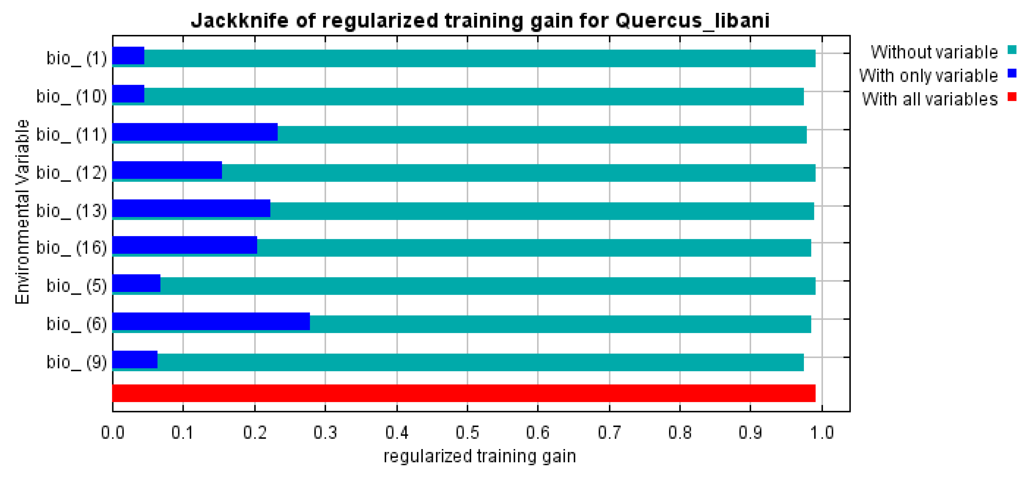
3.1. Statistical Analysis of Bioclimatic Variables

The variables, apart from the cluster sets created in the data space, were extracted from 19 bioclimatic variables used as the dataset in the study, and the KMO value was calculated as 0.65 for the remaining nine variables (Table 2). As this value was higher than the limit value required for factorizing the data cluster, a PCA was applied to the data.
Regarding the data groups created as a result of the PCA, nine bioclimatic variables forming the first two groups represented 95% of the total variance (Table 3). The first group in the reliability analysis, which had a Cronbach’s alpha value of 0.986 and was comprised of Bio1, Bio5, Bio6, Bio9, Bio10, and Bio11 was named the temperature group. The second group, which had a Cronbach’s alpha value of 0.767 and was comprised of Bio12, Bio13, and Bio16 was called the precipitation group. Figure 3 shows the components, rotated according to the varimax method.
The bioclimatic variables selected for the study in the QGIS 3.10.0 were uploaded to MaxEnt software and the current geographical distribution of Quercus libani Oliv. was modeled. In order to test the accuracy of the model, the AUC values of the training data and test data were analyzed (Figure 4). In terms of the AUC values, precise results were obtained for the training data with 0.91 and acceptable results were obtained for the test data with 0.83. The model was considered to be sensitive and descriptive. To determine the contribution of the bioclimatic variables, the Jackknife test option in the MaxEnt modeling program were used (Figure 5). This test revealed that the Bio6, Bio11, and Bio13 variables made a relatively higher contribution in the model. Moreover, all bioclimatic variables used in the model were understood to be necessary.

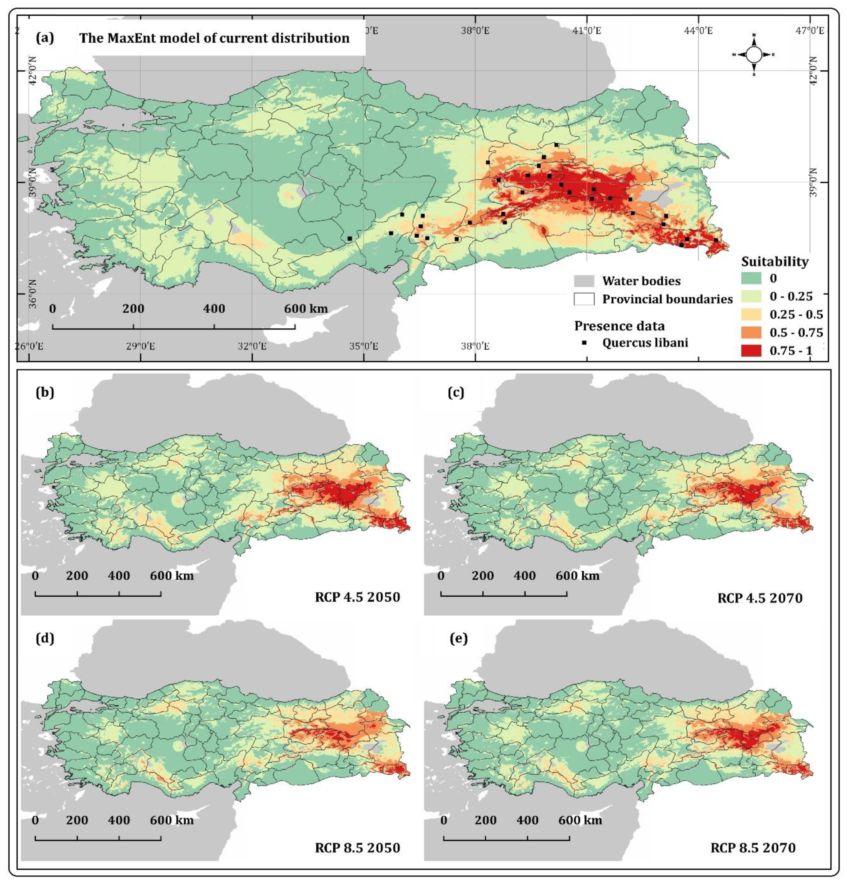
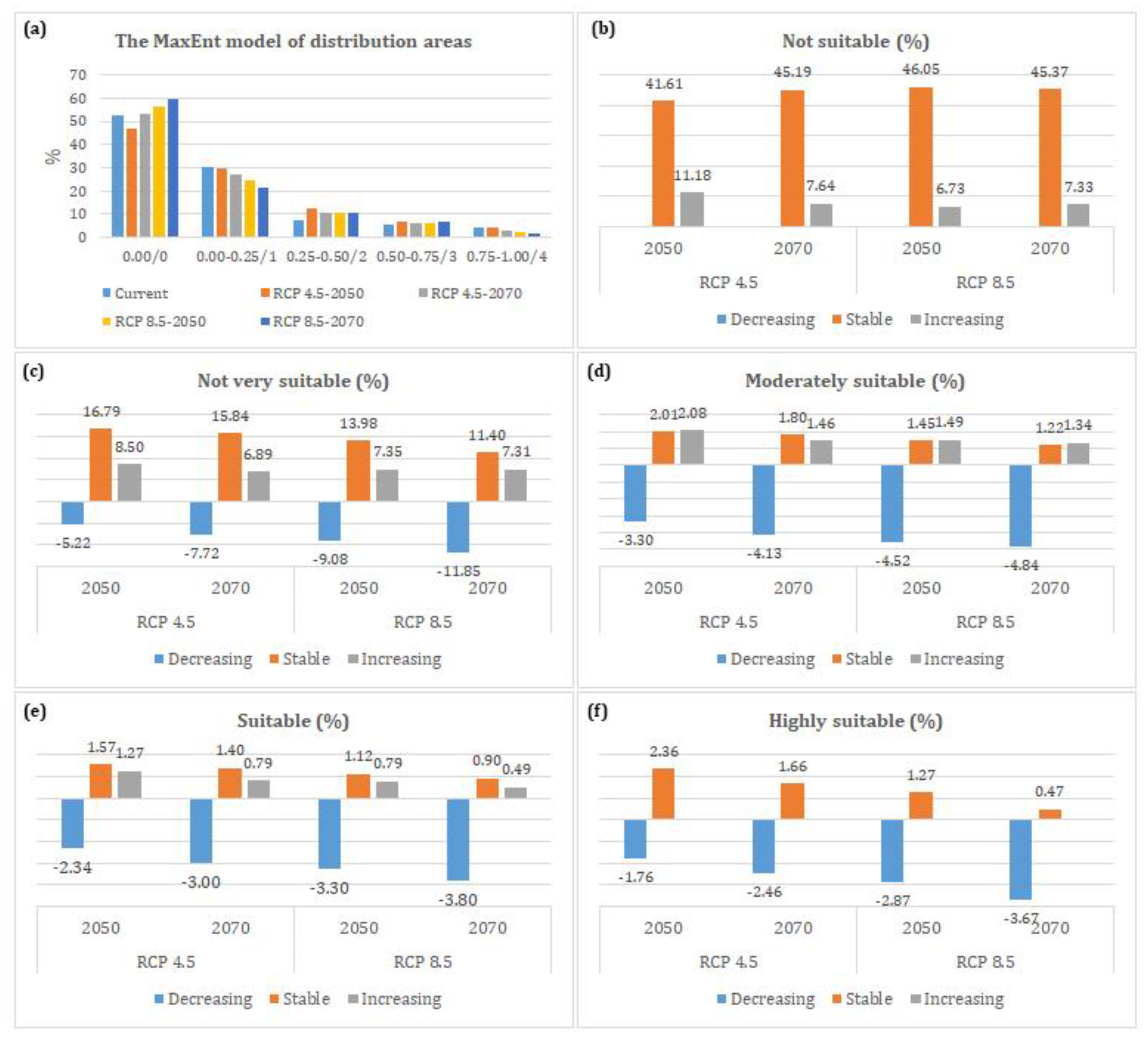
3.2. Current and Future Potential Geographical Distribution of Quercus Libani Olivier and Its Suitability According to Global Climate Change Scenarios

Figure 6 shows the current and future potential distribution of Quercus libani Oliv. under the global climate change scenarios RCP 4.5 and RCP 8.5 for 2050 and 2070. The model was classified into five levels (unsuitable to highly suitable) in the maps. The current and future potential distribution of Quercus libani Oliv. can be tracked on the maps. Table 4 shows the current and future distribution of this species according to the suitability classes on these maps.
According to the RCP 4.5 climate change scenario, there is no notable change by 2050, but there tends to be a decline in the potential geographical distribution of Quercus libani Oliv. by 2070. In the RCP 8.5 scenario, however, it will have a narrowing geographical distribution in 2050 and 2070. These predictions suggest that the geographical distribution of Quercus libani Oliv. will decrease in the future, while the possible habitat losses will be severe according to both scenarios.

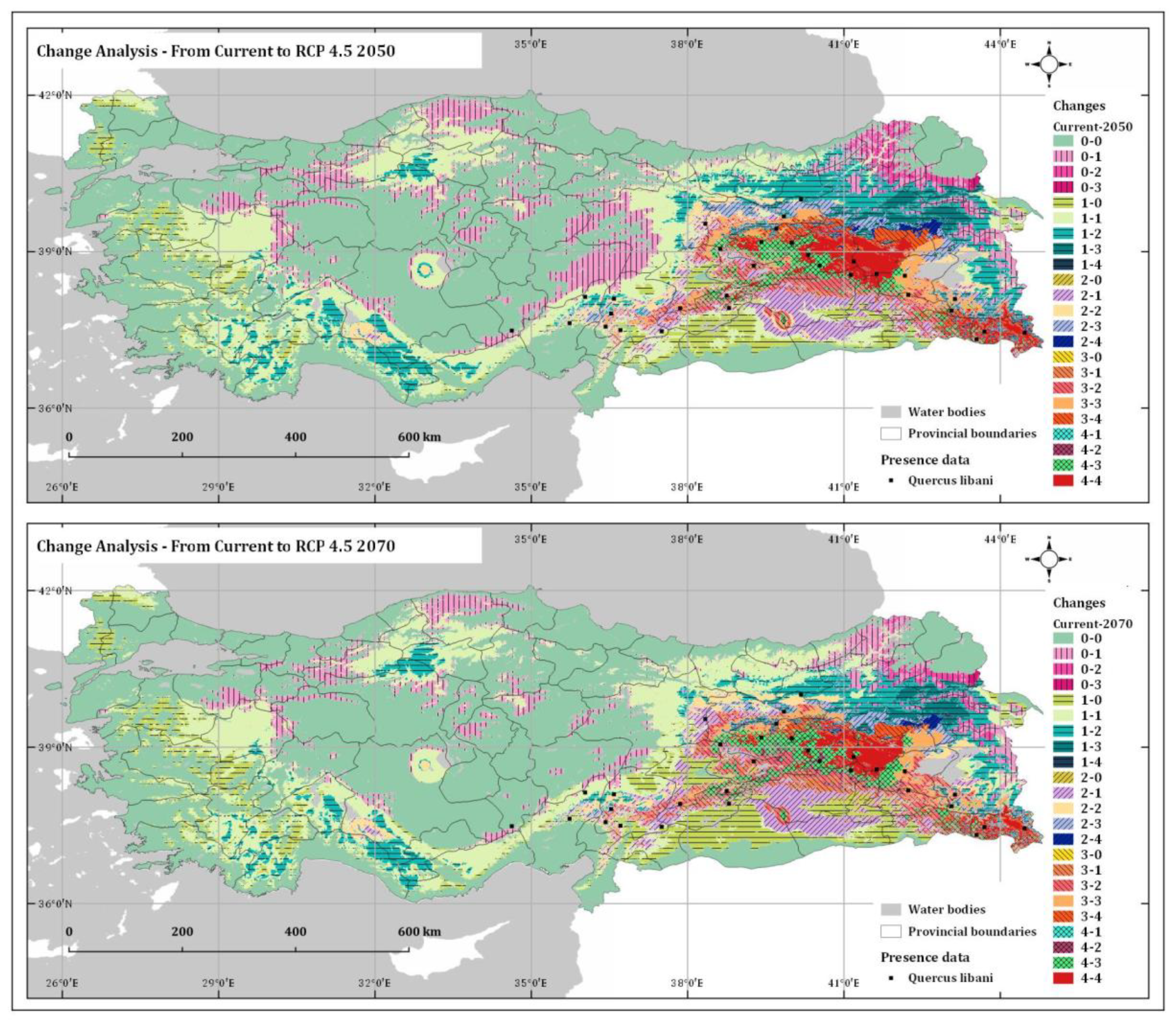
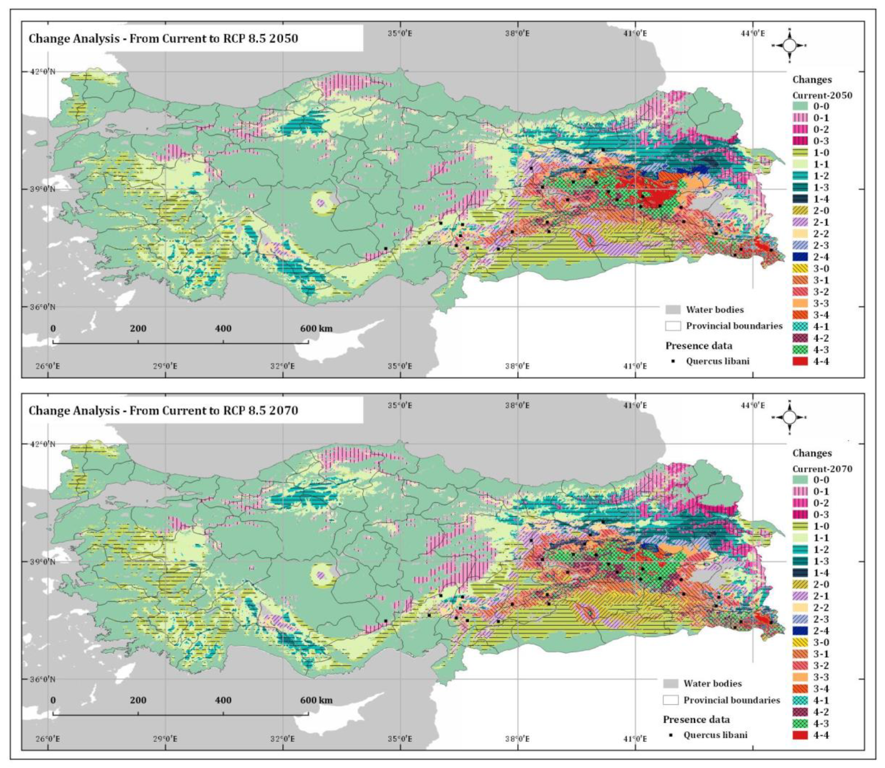
3.3. Changes from the Current Potential Geographical Distribution of Quercus libani Olivier

The changes were identified by comparing the current geographical distribution of Q. libani Oliv. with its predicted geographical distribution in 2050 and 2070 under the RCP 4.5 and RCP 8.5 climate scenarios (Figure 7 and Figure 8).
With the purpose of determining the changes, the data from two different time points were compared. The change was considered in two dimensions in this study. The spatial change was determined in the first dimension. The geographical distribution of the species was modeled for different time points and the spatial changes were indicated (Figure 7 and Figure 8). A spatial analysis of these changes was planned for the second dimension. To do so, the current potential geographical distribution of Q. libani Oliv. was classified. These classes, named suitability classes, show the potential geographical distribution for the species, from highly suitable ones to unsuitable ones. By using these classes, both the current and future potential geographical distribution according to the RCP 4.5 and RCP 8.5 climate scenarios in 2050 and 2070 were calculated. The changing geographical distribution areas from the present day to 2050 and 2070 were compared on the change maps, the change in the suitability classes was identified, and the surface areas of these changes were calculated. The codes that belong to current and future suitability were therefore compared. Due to the predicted geographical distribution, the direction and size of the changes were calculated (Table 5, Figure 9).

4. Discussion

As a result of global climate change, scientists have developed algorithms to provide useful data towards a better understanding the current distribution of plants and to help predict their future distribution areas based on several environmental variables [66,67]. MaxEnt is popular software based on maximum entropy [68,69,70]. In this study, the current and future distribution areas for Q. libani Oliv., a regional species in Turkey, were modeled using MaxEnt. Our results confirmed that the highly suitable area for this species is Eastern Anatolia [37,38,44]. However, in the 2050 and 2070 scenarios, Q. libani Oliv. will disappear if its distribution is limited to the current area of Southern Anatolia.
Bioclimatic variables predicting species distribution areas do not necessarily indicate the importance of topography. Topography plays a crucial role in the distribution of species in terms of its effect on the microclimate [71,72]. Related to the topography, there may be some suitable areas in adjacent countries like Persia, Syria, and Lebanon, but the distribution models for Turkey created in this study cannot provide information on them [73].
Although Q. libani Oliv. is an important oak species, there is limited research on it. Furthermore, we could not find any related research about its geographical distribution area in the recent literature. In this study, the occurrence of Q. libani Oliv. is predicted by determining not only the current geographical distribution, but also the impact of climate change on its future. For this prediction, we used MaxEnt software.
It is clear that the distribution areas and population of Q. libani Oliv. will change, but the nature of that change depends on the climate change scenario. Similar studies conducted on this topic also suggest that climate change is one of the most important factors that will affect habitat losses and fragmentation as well as the loss of biological diversity [16,19,74,75,76]. In terms of biogeography, such changes and as dislocations, population reductions, and species extinctions are perennial challenges [77,78,79].
The findings of the study show that the spatial distribution of this species will decrease by around 10% by 2070 according to the RCP 8.5 scenario. The proportion of highly suitable areas is estimated to decrease from 4% to 1.5% in the future.
Almost all bovine and ovine animals feed on oak leaves and acorns. Therefore, areas where oak species are present are considered to be the most suitable places for grazing [80]. The current distribution map demonstrates that this species is distributed in Hakkari, Şırnak, Van, Bitlis, Muş, Bingöl, Malatya, K. Maraş, Tunceli, and Elazığ, as well as Adıyaman, Diyarbakır, Batman, and Mardin provinces where livestock husbandry is the most important agricultural activity. Therefore, the species is under pressure from grazing. Excessive or unplanned grazing will further threaten the existence of this species in the future. For that reason, areas with young individuals and degraded stands should be protected.
There are 341 seed stands in Turkey, only 13 of which belong to oak species [81]. Out of these oak seed stands, there is only one for Q. libani Olivier. This number is insufficient and should be increased for Lebanon Oak. To this end, the habitat conditions of the existing stands should be identified, and the optimum ones retained, with some of them reserved as seed stands.
The RCP 4.5 scenario estimated that there will be no major changes in the geographical distribution of the species by 2050. However, there will be a decline in suitable and highly suitable areas by 2070. The results of the analysis made for the RCP 8.5 scenario show that the losses in terms of its geographical distribution are predicted to be severe. Although the prediction in this scenario does not indicate any marked change for 2050, there will be a major decrease in suitable and highly suitable areas by 2070.
As regards the direction of the changes expected to take place in the geographical distribution of Q. libani Oliv., only 4% of the currently unsuitable areas for its potential distribution will become suitable by 2050 according to the RCP 4.5. scenario, while 26% of the suitable areas will become unsuitable. By 2070, those rates will be 3% and 38%, respectively. By 2050, the rates will be 3.9% and 46%, respectively, and 4.6% and 56%, respectively, by 2070, according to the RCP 8.5 scenario. These rates indicate that the RCP 8.5 scenario envisions more severe consequences.

5. Conclusions

This study revealed that the geographical distribution areas of Q.libani Oliv. will be negatively affected by climate change according to a model based on the maximum entropy algorithm, and the suitable distribution areas will be narrower. Therefore, we suggest that the state forestry authority, which manages 99% of the forests in Turkey, should take precautions for the future. Moreover, it should be emphasized that land use plans should be developed and genetic studies should be supported to conserve seed sources for the continuity of the species and ensure the species’ transition to possible distribution areas in the future, apart from the protective measures put in place to prevent excessive grazing and consumption. Stands with Q. libani Oliv. individuals that are resistant to drought can be identified through genetic studies to ensure the continuity of the species and its resistance to climate change in the future. Therefore, efforts should be undertaken to conserve for the future for those individuals that will be less significantly affected by the negative impacts of climate change and can continue surviving and reproducing.

Author Contributions

Conceptualization, H.O.Ç. and Ö.K.Ö.; Methodology, Ö.K.Ö.; Software, Ö.K.Ö.; Validation H.O.Ç., Ö.K.Ö., and E.S.A.; Formal Analysis, Ö.K.Ö.; Investigation, H.O.Ç.; Resources, Ö.K.Ö. and E.S.A.; Data Curation, H.O.Ç. and Ö.K.Ö.; Writing—Original Draft Preparation, H.O.Ç., Ö.K.Ö., and E.S.A.; Writing—Review and Editing, E.S.A.; Visualization, Ö.K.Ö.; Supervision, H.O.Ç. All authors have read and agreed to the published version of the manuscript.

Funding

This research received no external funding.

Conflicts of Interest

The authors declare no conflict of interest.

References

  1. Adhikari, D.; Barik, S.; Upadhaya, K. Habitat distribution modelling for reintroduction of Ilex khasiana Purk., a critically endangered tree species of northeastern India. Ecol. Eng. 2012, 40, 37–43. [Google Scholar] [CrossRef] [Green Version]
  2. Barnosky, A.D.; Matzke, N.; Tomiya, S.; Wogan, G.O.; Swartz, B.; Quental, T.B.; Marshall, C.; McGuire, J.L.; Lindsey, E.L.; Maguire, K.C. Has the Earth’s sixth mass extinction already arrived? Nature 2011, 471, 51–57. [Google Scholar] [CrossRef] [PubMed]
  3. Lenoir, J.; Gégout, J.-C.; Marquet, P.; De Ruffray, P.; Brisse, H.J.S. A significant upward shift in plant species optimum elevation during the 20th century. Science 2008, 320, 1768–1771. [Google Scholar] [CrossRef] [PubMed]
  4. Bertrand, R.; Lenoir, J.; Piedallu, C.; Riofrío-Dillon, G.; de Ruffray, P.; Vidal, C.; Pierrat, J.-C.; Gégout, J.-C.J.N. Changes in plant community composition lag behind climate warming in lowland forests. Nature 2011, 479, 517–520. [Google Scholar] [CrossRef] [PubMed]
  5. Türkeş, M. Küresel iklim değişikliği nedir? Temel kavramlar, nedenleri, gözlenen ve öngörülen değişiklikler. İklim Değişikliği ve Çevre 2008, 1, 26–37. [Google Scholar]
  6. Worth, J.R.; Harrison, P.A.; Williamson, G.J.; Jordan, G.J. Whole range and regional-based ecological niche models predict differing exposure to 21st century climate change in the key cool temperate rainforest tree southern beech (N othofagus cunninghamii). Austral Ecol. 2015, 40, 126–138. [Google Scholar] [CrossRef]
  7. Liu, X.; Pan, Y.; Zhu, X.; Li, S. Spatiotemporal variation of vegetation coverage in Qinling-Daba Mountains in relation to environmental factors. Acta Geogr. Sin 2015, 5, 705–716. [Google Scholar]
  8. Wang, B.; Xu, G.; Li, P.; Li, Z.; Zhang, Y.; Cheng, Y.; Jia, L.; Zhang, J. Vegetation dynamics and their relationships with climatic factors in the Qinling Mountains of China. Ecol. Indic. 2020, 108, 105719. [Google Scholar] [CrossRef]
  9. IPCC. Climate Change 2014: Synthesis Report. Contribution of Working Groups I, II and III to the Fifth Assessment Report of the Intergovernmental Panel on Climate Change; IPCC: Geneva, Switzerland, 2014; p. 151. [Google Scholar]
  10. Chichorro, F.; Juslén, A.; Cardoso, P. A review of the relation between species traits and extinction risk. Biol. Conserv. 2019, 237, 220–229. [Google Scholar] [CrossRef]
  11. Ashraf, U.; Ali, H.; Chaudry, M.N.; Ashraf, I.; Batool, A.; Saqib, Z. Predicting the potential distribution of olea ferruginea in pakistan incorporating climate change by using maxent model. Sustainability 2016, 8, 722. [Google Scholar] [CrossRef] [Green Version]
  12. Cobben, M.M.P.; van Treuren, R.; Castaneda-Alvarez, N.P.; Khoury, C.K.; Kik, C.; van Hintum, T.J.L. Robustness and accuracy of Maxent niche modelling for Lactuca species distributions in light of collecting expeditions. Plant Genet. Resour.-C 2015, 13, 153–161. [Google Scholar] [CrossRef] [Green Version]
  13. Fitzpatrick, M.C.; Gove, A.D.; Sanders, N.J.; Dunn, R.R. Climate change, plant migration, and range collapse in a global biodiversity hotspot: The Banksia (Proteaceae) of Western Australia. Glob. Chang. Biol. 2008, 14, 1337–1352. [Google Scholar] [CrossRef]
  14. Lawler, J.J.; Shafer, S.L.; White, D.; Kareiva, P.; Maurer, E.P.; Blaustein, A.R.; Bartlein, P.J. Projected climate-induced faunal change in the Western Hemisphere. Ecology 2009, 90, 588–597. [Google Scholar] [PubMed] [Green Version]
  15. Thuiller, W.; Lavorel, S.; Araújo, M.B.; Sykes, M.T.; Prentice, I.C. Climate change threats to plant diversity in Europe. Proc. Natl. Acad. Sci. USA 2005, 102, 8245–8250. [Google Scholar] [PubMed] [Green Version]
  16. Yi, Y.J.; Cheng, X.; Yang, Z.F.; Zhang, S.H. Maxent modeling for predicting the potential distribution of endangered medicinal plant (H. riparia Lour) in Yunnan, China. Ecol. Eng. 2016, 92, 260–269. [Google Scholar] [CrossRef]
  17. Zhang, K.; Yao, L.; Meng, J.; Tao, J. Maxent modeling for predicting the potential geographical distribution of two peony species under climate change. Sci. Total Environ. 2018, 634, 1326–1334. [Google Scholar]
  18. Gaston, K.J. Species richness: Measure and measurement. Biodibersity: A Biology of Numbers and Difference; Blackwell Science: Hoboken, NJ, USA, 1996; pp. 77–113. [Google Scholar]
  19. Arslan, E.S. İklim değişimi senaryoları ve tür dağılım modeline göre kentsel yol ağaçlarının ekosistem hizmetleri bağlamında değerlendirilmesi: Robinia pseudoacacia L. örneği. Türkiye Ormancılık Dergisi 2019, 20, 142–148. [Google Scholar] [CrossRef] [Green Version]
  20. Phillips, S.J.; Dudik, M. Modeling of species distributions with Maxent: New extensions and a comprehensive evaluation. Ecography 2008, 31, 161–175. [Google Scholar] [CrossRef]
  21. Sarikaya, O.; Karaceylan, I.B.; Sen, I. Maximum Entropy Modeling (Maxent) of Current and Future Distributions of Ips Mannsfeldi (Wachtl, 1879) (Curculionidae: Scolytinae) in Turkey. Appl. Ecol. Environ. Res. 2018, 16, 2527–2535. [Google Scholar] [CrossRef]
  22. Sérgio, C.; Figueira, R.; Draper, D.; Menezes, R.; Sousa, A.J. Modelling bryophyte distribution based on ecological information for extent of occurrence assessment. Biol. Conserv. 2007, 135, 341–351. [Google Scholar] [CrossRef]
  23. Tittensor, D.P.; Baco, A.R.; Brewin, P.E.; Clark, M.R.; Consalvey, M.; Hall-Spencer, J.; Rowden, A.A.; Schlacher, T.; Stocks, K.I.; Rogers, A.D. Predicting global habitat suitability for stony corals on seamounts. J. Biogeogr. 2009, 36, 1111–1128. [Google Scholar] [CrossRef] [Green Version]
  24. Wang, Y.-S.; Xie, B.-Y.; Wan, F.-H.; Xiao, Q.-M.; Dai, L.-Y. The potential geographic distribution of Radopholus similis in China. Agric. Sci. China 2007, 6, 1444–1449. [Google Scholar] [CrossRef]
  25. Ward, D.F. Modelling the potential geographic distribution of invasive ant species in New Zealand. Biol. Invasions 2007, 9, 723–735. [Google Scholar] [CrossRef]
  26. Williams, J.N.; Seo, C.; Thorne, J.; Nelson, J.K.; Erwin, S.; O’Brien, J.M.; Schwartz, M.W. Using species distribution models to predict new occurrences for rare plants. Divers. Distrib. 2009, 15, 565–576. [Google Scholar] [CrossRef]
  27. Wollan, A.K.; Bakkestuen, V.; Kauserud, H.; Gulden, G.; Halvorsen, R. Modelling and predicting fungal distribution patterns using herbarium data. J. Biogeogr. 2008, 35, 2298–2310. [Google Scholar] [CrossRef]
  28. Yuan, H.S.; Wei, Y.L.; Wang, X.G. Maxent modeling for predicting the potential distribution of Sanghuang, an important group of medicinal fungi in China. Fungal Ecol. 2015, 17, 140–145. [Google Scholar] [CrossRef]
  29. Brito, J.C.; Acosta, A.L.; Álvares, F.; Cuzin, F. Biogeography and conservation of taxa from remote regions: An application of ecological-niche based models and GIS to North-African Canids. Biol. Conserv. 2009, 142, 3020–3029. [Google Scholar] [CrossRef]
  30. Elith, J.; Leathwick, J.R. Species distribution models: Ecological explanation and prediction across space and time. Annu. Rev. Ecol. Evol. Syst. 2009, 40, 677–697. [Google Scholar] [CrossRef]
  31. Wei, B.; Wang, R.L.; Hou, K.; Wang, X.Y.; Wu, W. Predicting the current and future cultivation regions of Carthamus tinctorius L. using MaxEnt model under climate change in China. Glob. Ecol. Conserv. 2018, 16. [Google Scholar] [CrossRef]
  32. Pearson, R.G.; Raxworthy, C.J.; Nakamura, M.; Townsend Peterson, A. Predicting species distributions from small numbers of occurrence records: A test case using cryptic geckos in Madagascar. J. Biogeogr. 2007, 34, 102–117. [Google Scholar] [CrossRef]
  33. Tsoar, A.; Allouche, O.; Steinitz, O.; Rotem, D.; Kadmon, R. A comparative evaluation of presence-only methods for modelling species distribution. Divers. Distrib. 2007, 13, 397–405. [Google Scholar] [CrossRef]
  34. Lv, X.; Zhou, G. Climatic suitability of the geographic distribution of Stipa breviflora in Chinese temperate grassland under climate change. Sustainability 2018, 10, 3767. [Google Scholar] [CrossRef] [Green Version]
  35. Wu, W.; Li, Y.; Hu, Y.; Xiu, C.; Yan, X. Impacts of changing forest management areas on forest landscapes and habitat patterns in northeastern China. Sustainability 2018, 10, 1211. [Google Scholar] [CrossRef] [Green Version]
  36. Dündar, T. Demirköy yöresi Istranca meşelerinin (Quercus hartwissiana Stev.) fiziksel özellikleri. İstanbul Üniversitesi Orman Fakültesi Dergisi 2001, 51, 65–80. [Google Scholar]
  37. GDF. Turkish Forestry Statistics. Available online: https://www.ogm.gov.tr/ekutuphane/Istatistikler/Forms/AllItems.aspx (accessed on 10 January 2020).
  38. Yaltırık, F. Manual for Identification of Turkish Oaks; General Directorate of Forestry Press: Eskişehir, Turkey, 1984. [Google Scholar]
  39. IUCN. The IUCN Red List of Threatened Species. Available online: https://www.iucnredlist.org/en (accessed on 11 January 2020).
  40. Stephan, J. The IUCN Red List of Threatened Species 2018. E.T194187A2303417, 11 September 2018. [Google Scholar]
  41. Grieve, M. A Modern Herbal; Courier Corporation: Chelmsford, MA, USA, 2013; Volume 2. [Google Scholar]
  42. Abrahami, A. Quercus Libani Jpg. Available online: https://upload.wikimedia.org/wikipedia/commons/0/07/Quercus_libani_port.jpg (accessed on 14 February 2020).
  43. Akkemik, Ü. Türkiye’nin doğal-egzotik ağaç ve çalıları I; Orman Genel Müdürlüğü Yayınları: Ankara, Turkey, 2014. [Google Scholar]
  44. Davis, P.H. Flora of Turkey and the East Aegean Islands—VIII; David, P.H., Ed.; Edinburgh University Press: Edinburgh, UK, 1984; Volume 8. [Google Scholar]
  45. GBIF. Global Biodiversity Information Facility. Available online: https://www.gbif.org/species/5293186 (accessed on 10 December 2019).
  46. Yaltırık, F. Türkiye Meşeleri Teşhis Kılavuzu; Tarım Orman ve Köyişleri Bakanlığı Genel Müdürlüğü Yayını: İstanbul, Turkey, 1984. [Google Scholar]
  47. QGis. QGis 3.8 Zanzibar—A Free and Open GIS. Available online: https://qgis.org/tr/site/forusers/download.html (accessed on 20 August 2019).
  48. WorldClim. WorldClim—Global Climate Data. Available online: www.worldclim.org (accessed on 20 August 2019).
  49. Hijmans, R.J.; Cameron, S.E.; Parra, J.L.; Jones, P.G.; Jarvis, A. Very high resolution interpolated climate surfaces for global land areas. Int. J. Climatol. J. R. Meteorol. Soc. 2005, 25, 1965–1978. [Google Scholar] [CrossRef]
  50. Moss, R.H.; Edmonds, J.A.; Hibbard, K.A.; Manning, M.R.; Rose, S.K.; Van Vuuren, D.P.; Carter, T.R.; Emori, S.; Kainuma, M.; Kram, T. The next generation of scenarios for climate change research and assessment. Nature 2010, 463, 747–756. [Google Scholar] [CrossRef]
  51. Remya, K.; Ramachandran, A.; Jayakumar, S. Predicting the current and future suitable habitat distribution of Myristica dactyloides Gaertn. Using MaxEnt model in the Eastern Ghats, India. Ecol. Eng. 2015, 82, 184–188. [Google Scholar] [CrossRef]
  52. Hunt, L.P.; Petty, S.; Cowley, R.; Fisher, A.; Ash, A.J.; MacDonald, N. Factors affecting the management of cattle grazing distribution in northern Australia: Preliminary observations on the effect of paddock size and water points1. Rangel. J. 2007, 29, 169–179. [Google Scholar] [CrossRef]
  53. CESM. Community Earth System Model (CESM)/CCSM4.0 Public Release. Available online: http://www.cesm.ucar.edu/models/ccsm4.0/ (accessed on 10 December 2019).
  54. Field, A. Discovering Statistics Using IBM SPSS Statistics; Sage: Thousand Oaks, CA, USA, 2013. [Google Scholar]
  55. Yurdugül, H. Faktör analizinde KMO ve Bartlett testleri neyi ölçer. Available online: http://yunus.hacettepe.edu.tr/~yurdugul/3/indir/Kuresellik.pdf (accessed on 10 January 2020).
  56. IBM. FACTOR does not print KMO or Bartlett test for Nonpositive Definite Matrices. Available online: https://www.ibm.com/support/pages/factor-does-not-print-kmo-or-bartlett-test-nonpositive-definite-matrices (accessed on 5 January 2020).
  57. Aït-Sahalia, Y.; Xiu, D. Principal component analysis of high-frequency data. J. Am. Stat. Assoc. 2019, 114, 287–303. [Google Scholar] [CrossRef] [Green Version]
  58. Phillips, S.J.; Anderson, R.P.; Schapire, R.E. Maximum entropy modeling of species geographic distributions. Ecol. Model. 2006, 190, 231–259. [Google Scholar] [CrossRef] [Green Version]
  59. Phillips, S.J. A brief tutorial on Maxent. AT T Res. 2005, 190, 231–259. [Google Scholar]
  60. Phillips, S.J.; Elith, J. POC plots: Calibrating species distribution models with presence-only data. Ecology 2010, 91, 2476–2484. [Google Scholar] [CrossRef] [PubMed]
  61. Zhao, D.; He, H.S.; Wang, W.J.; Wang, L.; Du, H.; Liu, K.; Zong, S. Predicting wetland distribution changes under climate change and human activities in a mid- and high-latitude region. Sustainability 2018, 10, 863. [Google Scholar] [CrossRef] [Green Version]
  62. Gassó, N.; Thuiller, W.; Pino, J.; Vilà, M. Potential distribution range of invasive plant species in Spain. NeoBiota 2012, 12, 25. [Google Scholar]
  63. Hosmer Jr, D.W.; Lemeshow, S.; Sturdivant, R.X. Applied Logistic Regression; John Wiley & Sons: Hoboken, NJ, USA, 2013; Volume 398. [Google Scholar]
  64. Shcheglovitova, M.; Anderson, R.P. Estimating optimal complexity for ecological niche models: A jackknife approach for species with small sample sizes. Ecol. Model. 2013, 269, 9–17. [Google Scholar] [CrossRef]
  65. Coban, H.O.; Koc, A.; Eker, M. Investigation on changes in complex vegetation coverage using multi-temporal landsat data of Western Black sea region—A case study. J. Environ. Biol. 2010, 31, 169–178. [Google Scholar]
  66. Yackulic, C.B.; Chandler, R.; Zipkin, E.F.; Royle, J.A.; Nichols, J.D.; Grant, E.H.C.; Veran, S. Presence-only modelling using MAXENT: When can we trust the inferences? Methods Ecol. Evol. 2013, 4, 236–243. [Google Scholar] [CrossRef]
  67. Thibaud, E.; Petitpierre, B.; Broennimann, O.; Davison, A.C.; Guisan, A. Measuring the relative effect of factors affecting species distribution model predictions. Methods Ecol. Evol. 2014, 5, 947–955. [Google Scholar] [CrossRef]
  68. Li, Y.; Li, M.; Li, C.; Liu, Z. Optimized maxent model predictions of climate change impacts on the suitable distribution of cunninghamia lanceolata in China. Forests 2020, 11, 302. [Google Scholar] [CrossRef] [Green Version]
  69. Nameer, P. The expanding distribution of the Indian Peafowl (Pavo cristatus) as an indicator of changing climate in Kerala, southern India: A modelling study using MaxEnt. Ecol. Indic. 2020, 110, 105930. [Google Scholar]
  70. Gebrewahid, Y.; Abrehe, S.; Meresa, E.; Eyasu, G.; Abay, K.; Gebreab, G.; Kidanemariam, K.; Adissu, G.; Abreha, G.; Darcha, G. Current and future predicting potential areas of Oxytenanthera abyssinica (A. Richard) using MaxEnt model under climate change in Northern Ethiopia. Ecol. Process. 2020, 9, 6. [Google Scholar] [CrossRef] [Green Version]
  71. Dobrowski, S.Z. A climatic basis for microrefugia: The influence of terrain on climate. Glob. Chang. Biol. 2011, 17, 1022–1035. [Google Scholar] [CrossRef]
  72. Çoban, H.O.; Çoşgun, S. The role of topography in the spatial distribution of tree species in the Mediterranean region of Turkey. Fresenius Environ. Bull. 2020, 29, 1369–1378. [Google Scholar]
  73. Luoto, M.; Heikkinen, R. Disregarding topographical heterogeneity biases species turnover assessments based on bioclimatic models. Glob. Chang. Biol. 2008, 14, 483–494. [Google Scholar] [CrossRef]
  74. Akyol, A.; Örücü, Ö.K. İklim Değişimi Senaryoları ve Tür Dağılım Modeline Göre Kızılcık Türünün (Cornus mas L.) Odun Dışı Orman Ürünleri Kapsamında Değerlendirilmesi. Avrupa Bilim ve Teknoloji Dergisi 2019, 224–233. [Google Scholar] [CrossRef]
  75. Qin, A.L.; Liu, B.; Guo, Q.S.; Bussmann, R.W.; Ma, F.Q.; Jian, Z.J.; Xu, G.X.; Pei, S.X. Maxent modeling for predicting impacts of climate change on the potential distribution of Thuja sutchuenensis Franch., an extremely endangered conifer from southwestern China. Glob. Ecol. Conserv. 2017, 10, 139–146. [Google Scholar] [CrossRef]
  76. Al-Qaddi, N.; Vessella, F.; Stephan, J.; Al-Eisawi, D.; Schirone, B. Current and future suitability areas of kermes oak (Quercus coccifera L.) in the Levant under climate change. Reg. Environ. Chang. 2017, 17, 143–156. [Google Scholar] [CrossRef]
  77. Peterson, A.T.; Papes, M.; Eaton, M. Transferability and model evaluation in ecological niche modeling: A comparison of GARP and Maxent. Ecography 2007, 30, 550–560. [Google Scholar] [CrossRef]
  78. Raxworthy, C.J.; Pearson, R.G.; Rabibisoa, N.; Rakotondrazafy, A.M.; Ramanamanjato, J.-B.; Raselimanana, A.P.; Wu, S.; Nussbaum, R.A.; Stone, D.A. Extinction vulnerability of tropical montane endemism from warming and upslope displacement: A preliminary appraisal for the highest massif in Madagascar. Glob. Chang. Biol. 2008, 14, 1703–1720. [Google Scholar] [CrossRef] [Green Version]
  79. Hughes, L. Biological consequences of global warming: Is the signal already apparent? Trends Ecol. Evol. 2000, 15, 56–61. [Google Scholar] [CrossRef]
  80. İnal, S. Meşe (Quercus) hakkında etimolojik ve tarihi etüdler. İstanbul Üniversitesi Orman Fakültesi Dergisi 1955, 5, 100–111. [Google Scholar]
  81. OGM. Tohum Meşcereleri. Available online: https://ortohum.ogm.gov.tr/SiteAssets/Sayfalar/Tohum-Mescereleri/Tohum%20Me%C5%9F%C3%A7ereleri(Adeti%20-Toplam%20alan).pdf (accessed on 10 January 2020).
Figure 1. Appearance (a) and leaves (b) of Quercus libani Olivier [42].
Sustainability 12 02671 g001
Figure 2. Geographical distribution of Quercus libani Olivier in the study area.
Sustainability 12 02671 g002
Figure 3. The data clusters in the principal component space.
Sustainability 12 02671 g003
Figure 4. Reliability test of the distribution model created for Quercus libani Olivier.
Sustainability 12 02671 g004
Figure 5. Jackknife test results of the variables in the model.
Sustainability 12 02671 g005
Figure 6. The current (a) and future potential geographical distribution of Quercus libani Olivier by 2050 and 2070 according to the climate scenarios RCP 4.5 (b,c) and RCP 8.5 (d,e). Suitability class range: 0 means not suitable, 0–0.25 means not very suitable, 0.25–0.5 means moderately suitable, 0.50–0.75 means suitable, and 0.75–1.0 means highly suitable for Quercus libani Olivier.
Sustainability 12 02671 g006
Figure 7. Changes from the current potential geographical distribution of Quercus libani Olivier to the RCP 4.5 climate scenario in 2050 and 2070 (0 means not suitable, 1 means not very suitable, 2 means moderately suitable, 3 means suitable, and 4 means highly suitable areas for Quercus libani Olivier. Number pairs with same code indicate no change and different codes in the number pairs indicate a change in both the area and the direction of the change.).
Sustainability 12 02671 g007
Figure 8. Changes from the current potential geographical distribution of Quercus libani Olivier to RCP 8.5 climate scenario in 2050 and 2070 (0 means not suitable, 1 means not very suitable, 2 means moderately suitable, 3 means suitable, and 4 means highly suitable areas for Quercus libani Olivier. Number pairs with the same code indicate no change and different codes in the number pairs indicate a change in both the area and the direction of the change.).
Sustainability 12 02671 g008
Figure 9. Graphs of change analysis for the current and future potential geographical distribution (a) of Quercus libani Oliv. under RCP 4.5 and RCP 8.5 climate scenarios. Changes in suitability classes (b) Not suitable, (c) Not very suitable, (d) Moderately suitable, (e) Suitable, and (f) Highly suitable.
Sustainability 12 02671 g009
Table 1. Characteristics of the sample points representing Quercus libani Olivier.
Point noLongitudeLatitudeProvinceDistrictElevation (m)Aspect (°)Slope (°)Precip.
(mm) *
Temp.
(°C) **
138°47’46”37°55’2”AdiyamanGerger876251155613.92
237°30’12”37°28’24”K. MarasPazarcık921164555614.67
338°37’52”39°3’23”MalatyaArapkir98869762312.93
437°51’27”37°54’54”MalatyaDoğanşehir995257653211.16
540°32’6”38°43’57”BingölGenç1037340783312.60
638°45’5”38°9’25”MalatyaPötürge10833221355412.58
743°32’50”37°19’9”HakkariÇukurca12293394380811.21
836°25’38”37°33’48”K. MarasAndırın1254350371011.19
939°16’11”38°43’51”ElazığMerkez13353341376211.58
1039°59’55”39°10’23”TunceliNazımiye1389100988410.48
1141°8’11”38°33’19”DiyarbakirKulp14143212291910.14
1235°44’12”37°37’49”AdanaKozan14611572365011.72
1342°14’14”38°10’17”SiirtŞirvan148116459368.84
1441°11’27”38°48’51”BingölSolhan15173268208.76
1536°42’44”37°29’46”K. MarasMerkez15321061065510.50
1639°25’2”39°11’11”TunceliHozat1545232168048.82
1743°3’55”37°52’13”VanÇatak1598178276978.91
1840°18’53”38°56’28”BingölMerkez1605130109629.55
1936°2’8”38°8’1”AdanaSaimbeyli1614225105257.45
2038°20’30”39°32’8”SivasDivriği16323331253010.08
2134°37’37”37°29’10”NigdeUlukışla1670356174139.28
2236°31’58”37°48’55”K. MarasGöksun170975366278.20
2339°42’24”39°26’37”TunceliPülümür1852193117765.38
2442°10’18”38°32’24”BitlisGüroymak187524488577.10
2536°35’20”38°5’55”K. MarasGöksun1902157155688.45
2644°28’12”37°26’48”HakkariŞemdinli1969187366297.87
2741°37’53”38°34’27”BitlisMutki1981178169198.52
2843°41’56”37°28’9”HakkariMerkez1996359437289.41
2940°10’50”40°0’14”ErzincanOtlukbeli2030336175934.23
3039°50’54”39°40’41”ErzincanÜzümlü2089328297064.64
3143°7’57”38°5’34”VanÇatak2557333426267.04
* Annual mean areal precipitation (Precip.) and ** annual mean temperature (Temp.) are the averages for the period 1970–2000 [48].
Table 2. Kaiser–Meyer–Olkin (KMO) and Bartlett’s test.
Kaiser–Meyer–Olkin Measure of Sampling Adequacy0.658
Bartlett’s Test of SphericityApprox. Chi-Square772.648
df36
Sig.0.000
Table 3. Factor loads of the variables in the rotated component matrix.
Data GroupVariableFactor LoadEigenvalueTotal VarianceCronbach’s AlphaCronbach’s Alpha If Item Deleted
Temperature 5.65562.8360.986
BIO10.997 0.980
BIO50.974 0.983
BIO100.974 0.982
BIO90.971 0.983
BIO60.955 0.985
BIO110.941 0.987
Precipitation 2.91432.3830.767
BIO160.989 0.440
BIO130.988 0.831
BIO120.963 0.743
Table 4. Spatial analyses of the current geographical distribution of Quercus libani Olivier and its future potential geographical distribution in 2050 and 2070.
Suitability Class/
Class Code *
Current RCP 4.5-2050RCP 4.5-2070RCP 8.5-2050RCP 8.5-2070
km2%km2%km2%km2%km2%
0.00/0412,062.252.9367,102.747.1415,646.353.3438,061.956.2464,108.359.5
0.00-0.25/1236,641.630.4233,703.330.0211,824.327.2192,469.524.7169,485.921.7
0.25-0.50/257,782.87.496,213.812.384,469.910.881,966.610.582,535.810.6
0.50-0.75/340,548.45.250,452.16.546,150.85.946,410.26.051,400.06.6
0.75-1.00/432,270.64.132,048.04.121,429.52.720,612.72.611,990.01.5
Total779,305.6100.0779,519.8100.0779,520.8100.077,9520.8100.0779,519.9100.0
* Class code: 0 means not suitable, 1 means not very suitable, 2 means moderately suitable, 3 means suitable, and 4 means highly suitable areas for Quercus libani Olivier.
Table 5. Changes from the current geographical distribution of Quercus libani Olivier to the predicted distribution in 2050 and 2070 according to RCP4.5 and RCP8.5 climate scenarios.
RCP 4.5RCP 4.5RCP 8.5RCP 8.5
Curr.2050Area (ha)Curr.2070Area (ha)Curr.2050Area (ha)Curr.2070Area (ha)
00326,070.200353,847.100359,914.20035,4740
0177,824.10151,937.30142,872.50140,358.3
029315.1027506.1029193.10213,537.4
03485.303402.303559.3033401.9
1040,932.61060,444.81070,965.71092,695.9
11131,585.911124,030.211109,255.81189,169.5
1254,713.21243,550.51241,776.51238,358.1
1311,856.91310,269.31314,643.11316,963.6
1434.714134.4141039.4141868.3
2063.8201891.7207609.72017,306.8
2125,8262130,465.42127,736.72120,540
2215,733.72214,131.92211,317.3229566.7
2312,659.3239382.4238147.7237822.5
243634.1242045.7243498.1242649.3
311842.6317599.63051.3301108.3
3216,509.53215,903.53113,745.73118,315.4
3312,329.23310,928.33211,9703210,318.7
349939.6346219.9338718.5337046.3
42550.1423941.5346139.5343822.7
4313,247.64315,352.74158.8411518.9
4418,468.14413,027.0427893.64210,958.6
4314,454.64316,227.6
449946443656.4
Total 783,621.4 783,011.4 781,507.1 781,950.9
Class code: 0 means not suitable, 1 means not very suitable, 2 means moderately suitable, 3 means suitable, and 4 means highly suitable areas for Quercus libani Olivier.

