Regional Differences in Fossil Energy-Related Carbon Emissions in China’s Eight Economic Regions: Based on the Theil Index and PLS-VIP Method

Abstract

Determining differences in regional carbon emissions and the factors that affect these differences is important in the realization of differentiated emissions mitigation policies. This paper adopts the Theil index and the partial least square-variable importance of projection (PLS-VIP) method to analyze the change characteristics, regional differences and causes of carbon emissions, as well as the extent to which various factors influenced carbon emissions in China’s eight economic regions in 2005–2017. The results indicate that (1) during the study period, carbon emissions in the eight economic regions displayed a rigid uptrend with a phased characteristic. The growth rates of carbon emissions were different across the studied regions. (2) The overall difference in regional carbon emissions showed an increasing trend, mainly owing to increasing interregional differences. (3) The extent of the influence and explanatory ability of each factor on regional carbon emissions and discrepancies in carbon emissions were different. Population size, economic development, and energy intensity were found to be the three main factors influencing regional carbon emission changes. Industrial structure and urbanization were also contributors to regional differences in emissions. The influence of energy structure on regional carbon emissions and its explanatory power were weak on the whole, but its elastic coefficients and VIP values changed significantly. Finally, regionally targeted proposals for emissions mitigation are offered.

1. Introduction

With continuous economic development and increasing consumption of fossil fuels, China became the largest carbon emitter worldwide in 2007 [1]. According to the British Petroleum (BP) Statistical Review of World Energy, China’s carbon emissions were responsible for nearly 27.3% of total global emissions in 2017, exceeding the sum of those of the US and EU. Meanwhile, resource shortages and environmental degradation have become the biggest challenges facing mankind. Whether or not the growth of China’s carbon emissions can be effectively controlled has become the focus of the Chinese government and the international community. Therefore, it is vital to find an effective emission reduction pathway in order to accomplish the goal of global carbon emissions reductions [1,2]. As the world′s largest developing country, at the World Climate Conferences in 2015, the Chinese government committed itself to reaching a peak of carbon dioxide emissions by 2030, to reduce carbon emissions per unit of GDP by 60–65% compared with the 2005 level, and to enhance the non–fossil fuels ratio of primary energy use by 20% [3]. However, the realization of this goal depends not only on the transformation and upgrading of traditional industries at the national level, including the optimization of energy consumption structures and the conversion of socio-economic development modes, but also on the formulation of targeted policies regarding energy conservation and emission reductions at the regional level. It should be pointed out that, due to China’s vast size, there are profound disparities in resource endowments, economic development levels, population scales, industrial structures and energy efficiencies across various regions or provinces (including municipalities and autonomous regions, collectively referred to as provinces) within China, leading to great differences in carbon emissions and their influencing factors [4,5,6,7]. Under these circumstances, it is of great import to determine the characteristics of carbon emissions in various provinces and their underlying driving factors. However, formulating a national emissions reduction policy based on provincial-level carbon mitigation will, on the one hand, increase the cost of policy making, and on the other, will increase the level difficulty of coordinating carbon emission reduction among provinces, thereby reducing the effectiveness of policy. Some scholars have taken three regions, i.e., Eastern, Central, and Western China as research units by which to analyze regional carbon emission differences and formulate national emission reduction policies [8,9]; however, we believe that this approach is flawed, as it is not nearly adequate to accurately understand the real situation of regional carbon emissions in China. To this end, to accurately reveal the characteristics and the main driving factors of China’s carbon emissions and formulate more targeted emissions reduction policies, it is necessary to select appropriate regions as research units. In the meantime, several questions should be answered in this respect. First, what are the characteristics of carbon emissions changes in different regions? Second, what are the major driving factors of regional carbon emissions in China, and how do these factors affect regional carbon emissions? Third, what are the differences of the drivers of carbon emissions across various regions? Judging from these, this paper takes China’s eight economic regions—as defined by the Development Research Center of the State Council based on similar levels of economic development—as its research object. Within the framework of national target emission reductions, we calculated the energy-related carbon emissions of these economic regions between 2006 and 2017 with updated terminal energy consumption data in every province of China and then broadly analyzed the features, regional disparities, and the main drivers of carbon emissions in each region.

Compared with previous research, our study contributes to the literature in three significant ways. First, selecting provinces with similar levels of economic development as research units (i.e., comprehensive economic regions) better reflects the features of energy-related carbon emissions changes in each economic region, and provides a more realistic description of current regional emissions in China, which lays a good foundation for the implementation of regionally targeted reductions of carbon emissions. Second, this study employed the Theil index approach, which can not only directly estimate the difference degree of carbon emissions in China’s eight economic regions, but can also decompose regional carbon emissions differences into two parts, i.e., inter- and intra-regional differences among different provinces, so as to reveal the direction and extent of their respective changes, as well as their role in the total difference, which helps to improve the accuracy of policy-making for regional-differentiated emissions reductions. Third, we want to have a more comprehensive understanding of carbon emissions and their effects in the eight economic regions of China. In order to achieve this, the PLS-VIP method was used. As far as we know, this approach has rarely been used in emissions analyses. Our data covered the years 2005–2017, which is important for capturing recent developments in region-level energy consumption and economic growth. This study will deepen our understanding of the drivers of carbon emissions in various regions in China. Additionally, it will also provide an important reference for other developing countries with large regional variations to reasonably formulate carbon emission mitigation policies.

2. Literature Review

2.1. Exploration of China’s Carbon Emissions

In recent years, there are plenty of studies on China’s carbon emission and it’s affecting factors. Clarke Sather et al. [10] and Yang et al. [11] used the variation coefficient, Gini coefficient, Lorenz curve, and Theil index to calculate the differences of carbon emission from energy consumption between China’s provinces or three regions of the eastern, central, and western regions from 1997 to 2007, and to estimate the contribution of each source of difference. Wang et al. [8] used the Shapley value algorithm to analyze the affecting factors of regional energy-related carbon emission differences in China. The decomposition results indicated that economic development, urbanization and energy structure can explain about 70% of the difference in regional carbon emissions, among which the imbalance of regional economic development is the main reason. Cheng et al. [12] and Liu et al. [13] employed spatial econometric approaches to analyze the spatial-temporal pattern, regional variation and their influencing factors of carbon emissions, noting that the energy intensity, energy structure, industrial structure, urbanization level and foreign direct investment (FDI) have significant effects on the spatial difference of carbon emissions. Among them, FDI has an inhibitory effect on carbon emissions in the central and eastern regions, while a promoting impact in the western region. Yang et al. [14], Wang et al. [15], Wang and Feng [16], and Jiang [17] employed an extended Log-Mean Divisia Index (LMDI) method to quantitatively analyze the influencing factors of China’s carbon emissions and to decompose the changes of carbon emissions into several components—namely, population size, economic development, energy structure, and energy intensity effect. They believed that economic growth is the most important factor affecting China’s carbon emissions, and regional differences in China’s carbon emissions mainly come from the intra-regional discrepancy. Zha et al. [18] used LMDI approach to investigate the driving forces of China’s urban-rural residential CO₂ emissions. Apart from these, a variety of studies discussed the drivers and mechanism of carbon emissions from regional and interprovincial perspectives. For example, Li et al. [19], Zhang et al. [20], Xiao et al. [21], Wang et al. [22], and Zhang et al. [23] adopted an improved STIRPAT (Stochastic Impacts by Regression on Population, Affluence, and Technology) model to explore the impacts of population, economy and technology on carbon emissions from China’s eastern, central, and western regions and individual province by principal component analysis or ridge regression method. The main findings demonstrated that energy intensity, energy structure, and economic growth are the main factors driving the change of carbon emissions. Zhou et al. [24] utilized the LMDI method to analyze the drivers of regional carbon emissions in China. By the LMDI approach, Jiang et al. [25] explored the driving forces of provincial carbon emissions. Shen et al. [26] decomposed the changes of carbon emissions in four development periods in Beijing. In addition, Liu [27] used a granger causality test to explore the relationship between GDP, energy consumption, and carbon emissions, pointing out that energy consumption has a significant positive effect on carbon emissions. By combining the province-level apparent energy consumption data with specific emission coefficient, Geng et al. [28] estimated CO₂ emissions of each province, and found that China’s coal-based energy structure and unique economic development had significant impacts on the emissions. Moreover, some other scholars studied the sectoral disparity and drivers on industrial carbon emissions in China’s economic regions and provinces [29,30]. For instance, Zhou et al. [31] analyzed the discrepancies of driving factors for industrial carbon emissions in 29 provinces.

On balance, the existing researches have made a lot of achievements in revealing spatial differences and driving forces of carbon emissions in China and provided many helpful policy implementations for effectively controlling carbon emissions and developing a low-carbon economy. However, the current studies present certain limitations due to the weakness of spatial scale and research methods. From the perspective of spatial research scale, the studies on regional differences of China’s carbon emissions and their affecting factors are mainly concentrated on four scales. First, three regions of East, Central, and West or four major economic plates of East, Central, West, and Northeast China were taken as the research unit [8,9], which can reflect the overall characteristics of China’s carbon emission spatial structure. However, the above-mentioned regional division appears to be too rough because of great differences in development conditions among them. Therefore, if we formulate national emission reduction policies based on this, it will inevitably produce “large and unified” and “one size fits all” for all regions. Second, according to the two indicators of carbon emission and its efficiency, some scholars divided China’s mainland 30 provinces (excluding Tibet) into four categories of regions (i.e., high emission–high efficiency region, high emission–low efficiency region, low emission–high efficiency region, and low emission–low efficiency region) by mean clustering algorithm and took them as research units to explore the regional differences in carbon emissions [32]. This method can effectively distinguish the discrepancy in the influence degree of each driver on carbon emissions in various regions, but it cuts the spatial linkage between economic development and carbon emissions among neighboring provinces. Third, provinces, cities, or counties were taken as the basic research units [33,34,35,36]. Although it can clearly represent the carbon emission characteristics of a single province (city, or county), it cuts off the economic links between provinces (city, or county) and ignores the existence of intra-regional carbon emission transfers. In this context, we make the national emission reduction policy based on the province (city, or county), it will not only raise the cost of policy-making, but also increase the coordination difficulty among the provinces (cities, or counties), thus affecting the effectiveness of the policy and ultimately leading to the failure of the overall national carbon emission reduction goal. The fourth is to study the regional differences, pattern evolution, and transfer characteristics of carbon emissions based on the eight regions divided by China’s input–output table [37,38]. However, the reasons for the regional emissions differences and the impacts of various factors on carbon emissions in different regions have not been thoroughly analyzed and accurately explained.

2.2. Emissions Research Methodologies

From the perspective of research methods of influencing factors on carbon emissions, many scholars adopted the environmental Kuznets curve (EKC) [39], Gini coefficient, Kaya identity [40] and LMDI [41], structural decomposition analysis (SDA) [42], or spatial econometric model [12] as their research methods. Although the above methods have widespread applications in the in-depth studies on regional carbon emissions differences and the factors driving energy-related carbon emissions, undoubtedly, there are still some deficiencies in the applicability of each method. For example, Gini coefficient does not have decomposability when estimating regional differences, so it is difficult to analyze the main sources of overall differences. The LMDI method can realize no residual decomposition, but it is known to have limitations in examining the elasticity of each explanatory variable (in other words, when other factors remain unchanged, the change of given factors will cause carbon emissions change) and separating the effects of various factors [43]. Although Kaya identity has been widely used to study carbon emission drivers, it is bound by the necessity of identity when decomposing various factors year by year. SDA carries out decomposition based on the assumption that the alternative elasticity between the factors is zero, and there are more subjective components in parameter estimation, thus it is not suitable applied in carbon emission driver analysis. SDA cannot be conducted multiplicatively [44,45]. Moreover, concerning the spatial panel data econometric method, there is usually an assumption that the explanatory variables are independent of each other, and thus making it difficult to eliminate the collinearity between explanatory variables. Therefore, the above methods may lose their effects in the real applications. Different from the above-mentioned methods, however, when the Theil index estimates the regional differences, it can divide the overall differences into two parts: the inter-regional and the intra-regional differences, and measure the contribution of each part to the overall differences, so as to reveal the main sources of the overall differences. Besides, the partial least square variable importance of projection (PLS-VIP) approach integrates the advantages of multiple linear regressions, canonical correlation analysis and principal component analyses, which can not only overcome the multicollinearity problem among explanatory variables, but also achieve the minimum mean square error with fewer factors than principal component regression. Particularly, it can accurately measure the importance of different explanatory variables on the dependent variable by using a variable importance of projection (VIP) value.

Given the above analysis, this paper calculates energy-related carbon emissions in China’s eight economic regions from 2005 to 2017 by using final energy consumption data of each province, and then uses the Theil index to extensively discuss the characteristics and differences of regional carbon emissions and the causes of these differences. Finally, we adopt the PLS-VIP method to quantitatively explore the influence of various driving factors on carbon emissions in each economic region.

3. Methods

3.1. Econometric Model of Carbon Emissions

Many studies have shown that regional carbon emission is not only affected by the economic development level, energy intensity, and population size but also by regional energy structure, industrial structure, and urbanization [46,47]. As China is currently in the stage of industrial restructuring, energy structure optimization and rapid urbanization, in our study, we add the three variables of industrial structure, energy structure and urbanization into the STIRPAT model. After taking natural logarithms, the extended STIRPAT model of carbon emissions is

$$\begin{gathered} ln{C}_{ij}={\alpha }_0+{\alpha }_{1}ln{P}_{ij}+{\alpha }_{2}ln{A}_{ij}+{\alpha }_{3}ln{T}_{ij}+{\alpha }_{4}ln{E}_{ij}+{\alpha }_{5}ln{S}_{ij} \\ +{\alpha }_{6}ln{U}_{ij}+ln{\epsilon }_{ij} \end{gathered}$$

(1)

In the formula, the subscript $i$ and $j$ denote the $i$th economic region in China and the $j$th year, respectively; $C$ represents carbon emission (mean value of all provincial carbon emissions in this economic region, 10⁴ ton); ${\alpha }_0$ indicates a constant; $P$ denotes year-end total population (10⁴ units); $A$ represents real GDP per capita (yuan); $T$ means energy intensity (energy consumption divided by GDP, tce per 10 thousand yuan); $E$ indicates energy structure (coal consumption divided by total primary energy consumption, %); $S$ represents industrial structure (output value of the secondary industry divided by total GDP, %); $U$ is urbanization rate (urban population divided by total population, %); $\epsilon$ is the random error term. ${\alpha }_1~{\alpha }_6$ are the elastic coefficients, indicating the change degree of carbon emission caused by 1% change of each explanatory variable.

Considering the possibility of the inverted U-shaped relationship between economic development and regional carbon emissions of China, we decompose the economic development level ${\alpha }_{2}ln{A}_{ij}$in the Formula (1) into the terms of ${\alpha }_{21}ln{A}_{ij}$ and the square term of its natural logarithm ${\alpha }_{22}{\left(\ln A_{ij}\right)}^2$. By calculating the first partial derivative of $ln{A}_{ij}$, we get the elasticity coefficient of GDP per capita to carbon emission: $\beta ={\alpha }_{21}+{\alpha }_{22}ln{A}_{ij}$. When the ${\alpha }_{22}$ is less than 0, it means that there is an EKC in this region; otherwise, there is no EKC. Consequently, Equation (1) can be written as follows:

$$\begin{gathered} ln{C}_{ij}={\alpha }_0+{\alpha }_{1}ln{P}_{ij}+{\alpha }_{21}ln{A}_{ij}+{\alpha }_{22}{\left(ln{A}_{ij}\right)}^2+{\alpha }_{3}ln{T}_{ij}+{\alpha }_{4}ln{E}_{ij} \\ +{\alpha }_{5}ln{S}_{ij}+{\alpha }_{6}ln{U}_{ij}+ln{\epsilon }_{ij} \end{gathered}$$

(2)

For the above model, we believe that the increases in population, the secondary industry proportion, coal consumed proportion in primary energy, and energy intensity will cause a rise in demand for energy consumption, which leads to an increase in carbon emissions. Accordingly, the values of ${\alpha }_1$, ${\alpha }_3$, ${\alpha }_4$ and ${\alpha }_5$ in Equation (2) are expected to be positive. In addition, according to the description from EKC, the carbon emission will first increase and then decrease with the increase of GDP per capita, so it is estimated that the value of ${\alpha }_{21}$ is positive, while that of ${\alpha }_{22}$ is negative. Furthermore, urbanization is an important factor affecting energy demand. Although the agglomeration effect of urbanization will reduce the carbon emission of energy consumption, in the early stage of the extensive urbanization process, the cement demand driven by infrastructure investment needs to consume a lot of energy, so the increase of urbanization rate will also lead to the growth of carbon emission. Thus, the value of ${\alpha }_6$ is expected to be positive.

3.2. Theil Index

Theil index was the first important indicator to measure regional differences in economic development levels. Compared with Gini coefficient, when estimating regional differences, Theil index can easily decompose the regional overall difference $\left(T\right)$ into two parts: inter-regional difference $\left(T_{WB}\right)$ and intra-regional difference between different provinces $\left(T_{WR}\right)$, thus analyzing their contribution to the total differences and the main sources of the overall differences [48]. According to this theory, we choose Theil index as an indicator to measure regional differences in carbon emissions of China’s eight main economic regions. The expression of Theil index after decomposing is as below:

$$T={\displaystyle \sum }_{i=1}^n{v}_i\left[{\displaystyle \sum }_{j=1}^m{v}_{ij}ln\left(\frac{v_{ij}}{d_{ij}}\right)\right]+{\displaystyle \sum }_{i=1}^n{v}_{i}ln\left(\frac{v_i}{d_i}\right)=T_{WR}+T_{WB}$$

(3)

In the formula, $n$ and $m$ respectively are the number of economic regions and the number of provinces within the region; $v_i$ represents the proportion of carbon emissions of region $i$ in China’s total emissions, $v_{ij}$ indicates the proportion of j provincial carbon emissions within region $i$ in China’s total carbon emissions; $d_i$ denotes the proportion of GDP of region $i$ in the total GDP of China, and $d_{ij}$ denotes the proportion of $j$ provincial GDP within region $i$ in China’s total GDP. The larger the Theil index, the greater the regional difference in the carbon emissions; the smaller the Theil index, the smaller the regional difference in the carbon emissions. In order to reveal the contribution of different sources, the quotient of inter-regional difference and overall difference ($T_{WR}/T$) is taken as the contribution rate between regions, and the quotient of intra-regional difference and overall difference ($\left(T_{WR}/T\right)$ is taken as the contribution rate within a region.

3.3. PLS-VIP Method

Partial least square (PLS) is a statistical tool relating the predictor (X) and response (Y) datasets through a multivariate linear equation that can model data in the cases of multi-collinearity and the number of instances being not more than the number of predictor variables. In this study, there has a single response variable y, the PLS regression model with h potential variables can be written as follows [49]:

$$\mathrm{X}=\mathrm{T}\mathrm{P}\prime +\mathrm{E}$$

(4)

$$\mathrm{y}=\mathrm{TQ}+\mathrm{f}$$

(5)

where $X\left(n\times p\right)$ indicates the matrix of predictor variable, $T\left(n\times h\right)$ indicates the X-score matrix of potential variable, $P\left(p\times h\right)$ represents the matrix of X-loadings, y$\left(n\times 1\right)$ represents the matrix of response variable, Q$\left(n\times 1\right)$ is the PLS regression coefficient, and $E\left(n\times p\right)$ and $f\left(n\times 1\right)$ are, respectively, the residual terms of X and y. To maximize the covariance between T and y, generally, we use a nonlinear iterative method to extract each score through deflating X (the score of response variable does not need to be extracted, because there is only one y-variable) until all variances in the datasets are explained. At the same time, the VIP scores, which are evaluated in the light of the output variables influenced by the potential spatial predictors, are used to determine the variable importance. The VIP score of the $j$th predictor variable to the response variable can be defined as [50]

$$VI{P}_j=\sqrt{p{\displaystyle \sum }_{h=1}^m{r}_h^2\left(Y;t_h\right)w_{hj}^2/{\displaystyle \sum }_{h=1}^m{r}_h^2\left(Y;t_h\right)}$$

(6)

where $p$ is the number of input variables, $w_{hj}$ is the weight of the $j$th variable on the latent variable$t_h$, which is used to evaluate the marginal contribution of $x_j$ to the construction of $t_h$ latent variable; $r_h\left(Y;t_h\right)$ indicates the explanatory ability of the $h$th latent variable to the response y-variable. The average of the squared VIP-scores is 1. In most cases, researchers regard the greater-than-one rule as the criterion of variable selection. However, Chong and Jun [51] believed that an appropriate threshold should range from 0.83 to 1.21. For this study, $VI{P}_{\mathrm{j}}>1$ indicates that the $j$th variable is a very important driver, $0.8<VI{P}_{\mathrm{j}}<1.0$ indicates that the $j$th variable is an important driver; whereas $0<VI{P}_j<0.8$ represents that the $j$th variable is an unimportant driver. The calculation process of PLS-VIP was completed with Umetrics SIMCA14.1 software (https://webshop.umetrics.com).

4. Empirical Results and Discussion

4.1. Division of Economic Regions

This study explores the regional differences in China’s carbon emissions from energy consumption and their driving factors. To identify the effects of inter-regional difference and intra-regional difference further on regional overall difference, we followed the method of the Development Research Center of China State Council that divided the 31 provinces in mainland China into eight main economic regions according to the following nine principles [52]: (i) spatially adjacent, (ii) similar natural conditions and resource endowment, (iii) similar level of economic development, (iv) closely related in economy or face similar development problems, (v) similar social structures, (vi) appropriate block size, (vii) due consideration of historical continuity, (viii) maintaining the integrity of the district, and (ix) facilitate regional research and policy analysis. The specific information on the eight main economic regions is given in

Table 1. Detailed information on China’s eight economic regions.

Economic Regions	Acronyms for Regions	Provinces Included in the Region	Regional Characteristics
Northeast economic region	NEER	Heilongjiang, Liaoning, Jilin	Natural conditions and resource endowment are similar. At present, there are many common problems, such as resource exhaustion, industrial structure upgrading and so on.
Northern coastal economic region	NCER	Beijing, Tianjin, Hebei, Shandong	With superior geographical location, convenient transportation, advanced science, technology, education and culture, it has made remarkable achievements in opening up.
Eastern coastal economic region	ECER	Shanghai, Jiangsu, Zhejiang	Modernization started early, with close economic ties with foreign countries in history. It has taken the lead in many areas of reform and opening up. It has rich human capital and obvious development advantages.
Southern coastal economic region	SCER	Fujian, Guangdong, Hainan	Facing Hong Kong, Macao and Taiwan, overseas social resources are rich and the degree of opening up is high.
Economic region in the middle reaches of the Yellow River	ERMRYR	Shaanxi, Shanxi, Henan, Inner Mongolia	Natural resources, especially coal and natural gas resources, are rich. It has an important strategic position, lack of opening-up, and arduous task of structural adjustment.
Economic region in the middle reaches of the Yangtze River	ERMRYTR	Hubei, Hunan, Jiangxi, Anhui	The agricultural production conditions are good, the population is dense, the degree of opening to the external world is low, and the pressure of industrial transformation is great.
Southwest economic region	SWER	Yunnan, Guizhou, Sichuan, Chongqing, Guangxi	It is located in a remote area with poor land and a large number of poor people. It has good conditions for opening up to South Asia.
Northwest economic region	NWER	Gansu, Qinghai, Ningxia, Xinjiang, Tibet	The natural conditions are bad, the land is vast, and the population is sparse, the market is narrow and small, and there are certain conditions for opening to the surrounding areas.

.

4.2. Carbon Emission Estimation and Data Sources

Due to the lack of official data on provincial CO₂ emissions in China, we used a reference approach suggested by the IPCC (2006) [53] to calculate provincial carbon emissions (In this study, Tibet is not included because of the lack of data) between 2005 and 2017. The computing formula is as below:

$$\mathrm{C}={\displaystyle \sum }_{\mathrm{j}=1}^8{\mathrm{C}}_{\mathrm{j}}={\displaystyle \sum }_{\mathrm{j}=1}^8{\mathrm{E}}_{\mathrm{j}}\times {\mathrm{SCC}}_{\mathrm{j}}\times {\mathrm{F}}_{\mathrm{j}}\times {\mathrm{CEC}}_{\mathrm{j}}\times 44/12$$

(7)

where C represents provincial energy-related carbon emissions;$E_j$ denotes the final consumption of the jth fossil energy type; $SC{C}_j$ represents the standard coal conversion coefficient of the jth fossil energy type; $F_j$ is the carbon oxidation factor of the jth fossil energy type (assuming complete oxidation, $F_j=1$); $CE{C}_j$ is the carbon emission coefficient of the jth fossil energy type, and 44/12 represents the molecular mass. The values of the above parameters were derived from the IPCC guidelines for national greenhouse gas inventories in 2006.

The terminal energy consumption data of eight major fossil fuels (i.e., raw coal, coke, crude oil, kerosene, diesel oil, gasoline, fuel oil, and natural gas) in every sample province come from China Energy Statistical Yearbooks (2006–2018) [54]. The socio-economic data (including population, urbanization level, GDP per capita, industrial value, and total GDP) of each province are acquired from the China Statistical Yearbook (2006–2018) [55] published by the National Bureau of Statistics of China. During the study period, in order to avoid the influence of price fluctuations, both nominal GDP and industrial values are converted to constant prices in 2005. The energy consumption is converted into standard coal based on the coefficient of conversion.

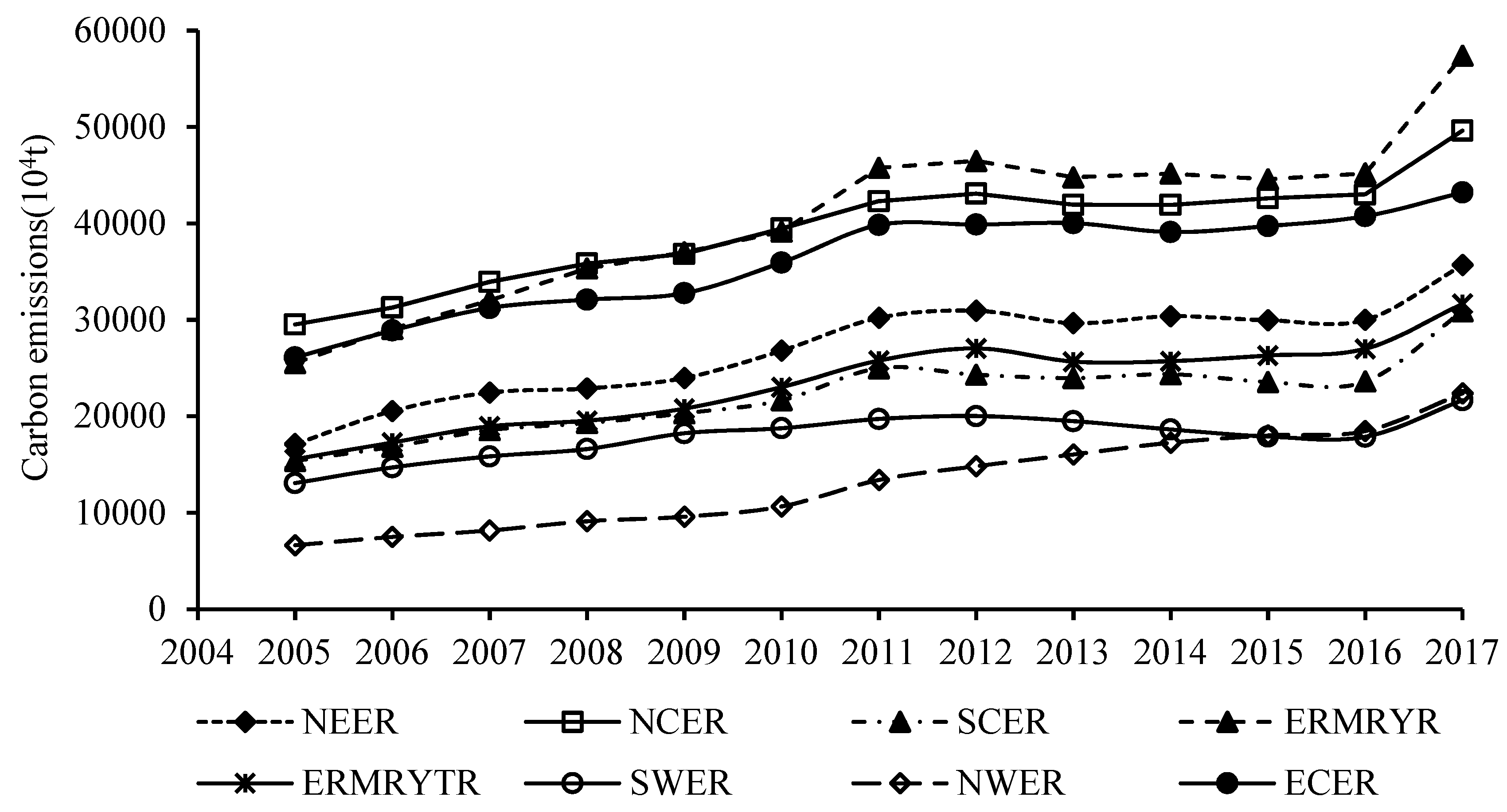
4.3. Characteristics of Carbon Emissions in China’s Eight Economic Regions

Figure 1 displays the carbon emissions and their changing trends of eight economic regions in China. From the perspective of carbon emissions, during the entire examined period (2005–2017), the top three emitters ranked as the economic region in the middle reaches of the Yellow River (ERMRYR), the northern coastal economic region (NCER), the eastern coastal economic region (ECER), and the northeast economic region (NEER). This indicates that those regions need to make more efforts to mitigate carbon emissions in the near future. Interestingly, the carbon emissions of the northwest economic region (NWER) and the southwest economic region (SWER) were always at the bottom, whereas emissions in regions such as the NEER, the economic region in the middle reaches of the Yangtze River (ERMRYTR) and the southern coastal economic region (SCER) were at medium levels. From the perspective of the change process, it can be found that all regions’ carbon emissions displayed an uptrend and experienced an obvious stage characteristic of “first rise–then fall–then rise” from 2005 to 2017 (notably, carbon emissions in the NWER continued to rise). That is to say, the carbon emissions of most regions showed an upward trend around 2012, then declined slightly, and then rose sharply again since 2016. Macro-control policies and economic growth fluctuation may explain why the regional carbon emissions overall displayed a firstly rise, then descending and then rise tendency. First, since 2005, owing to the improvement of international economic situation and the influence of macro-control policies, such as the continuous expansion of domestic demand and national “Four Trillion Yuan Stimulus Plan,” a great quantity of energy-intensive consumption industries and repetitive infrastructure projects have been launched, causing an obvious growth of energy consumption. Because the carbon emissions mainly come from fuel combustion, the carbon emissions in various regions reached a peak value around 2012, which also indirectly supported Guan et al.’s conclusion that China’s carbon dioxide emissions peaked in 2013 [56]. Second, in the 12th Five-Year-Plan (FYP), with the steady growth of the national economy and the gradual implementation of energy conservation and emission reduction and low-carbon strategy, carbon emissions in most regions began to fall. However, since the 13th FYP, China’s economy has actively adapted to and led the “new normal,” showing an overall trend of steady growth. Especially in 2017, in the context of the global economic downturn, China’s economic growth was strong, with GDP growth in the first three quarters respectively reaching 6.9%, 6.9% and 6.8%, higher than the expected goal of 6.5% in the whole year. Besides, economic growth was the most important factor stimulating carbon emissions growth. The above reasons ultimately resulted in rapid carbon emissions increase in all regions and a peak in 2017.

In terms of the change range, the growth rates of carbon emissions varied between economic regions. In all regions, the largest increase occurred in the NWER, in which carbon emissions rose from 66.25 million tons in 2005 to 223.83 million tons in 2017, with a mean annual increment of 18.30%. This implied that the emissions reduction in this region did not seem to be effective during the research period. The next were the ERMRYR, the NEER, the ERMRYTR, and the SCER, with an average annual increase of 9.60%, 8.34%, 7.96%, and 7.77%, respectively, whereas the increase in carbon emissions of the NCER, the SWER, and the ECER were very close and showed a relatively low level, with a mean annual increase of 5.23%, 5.06%, and 5.04%, respectively. In consideration of the heterogeneity of China’s regional carbon emissions, we must consider this disparity and its influencing factors in future emission reduction measures.

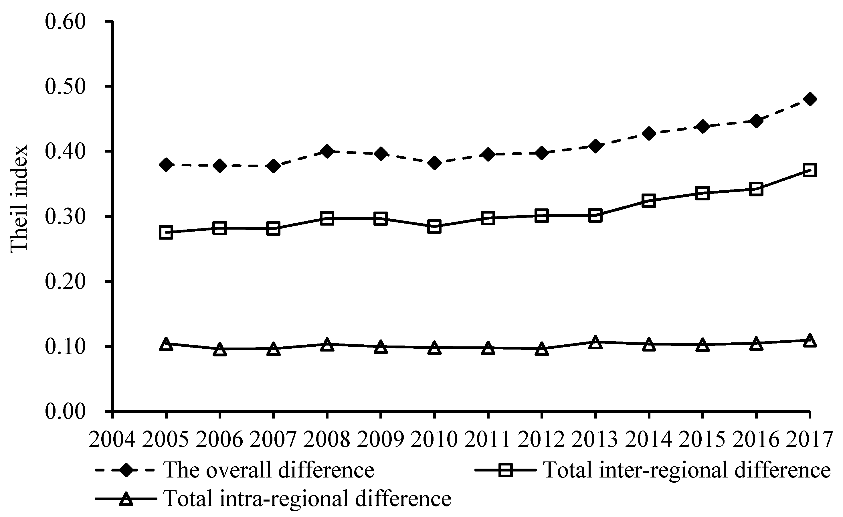
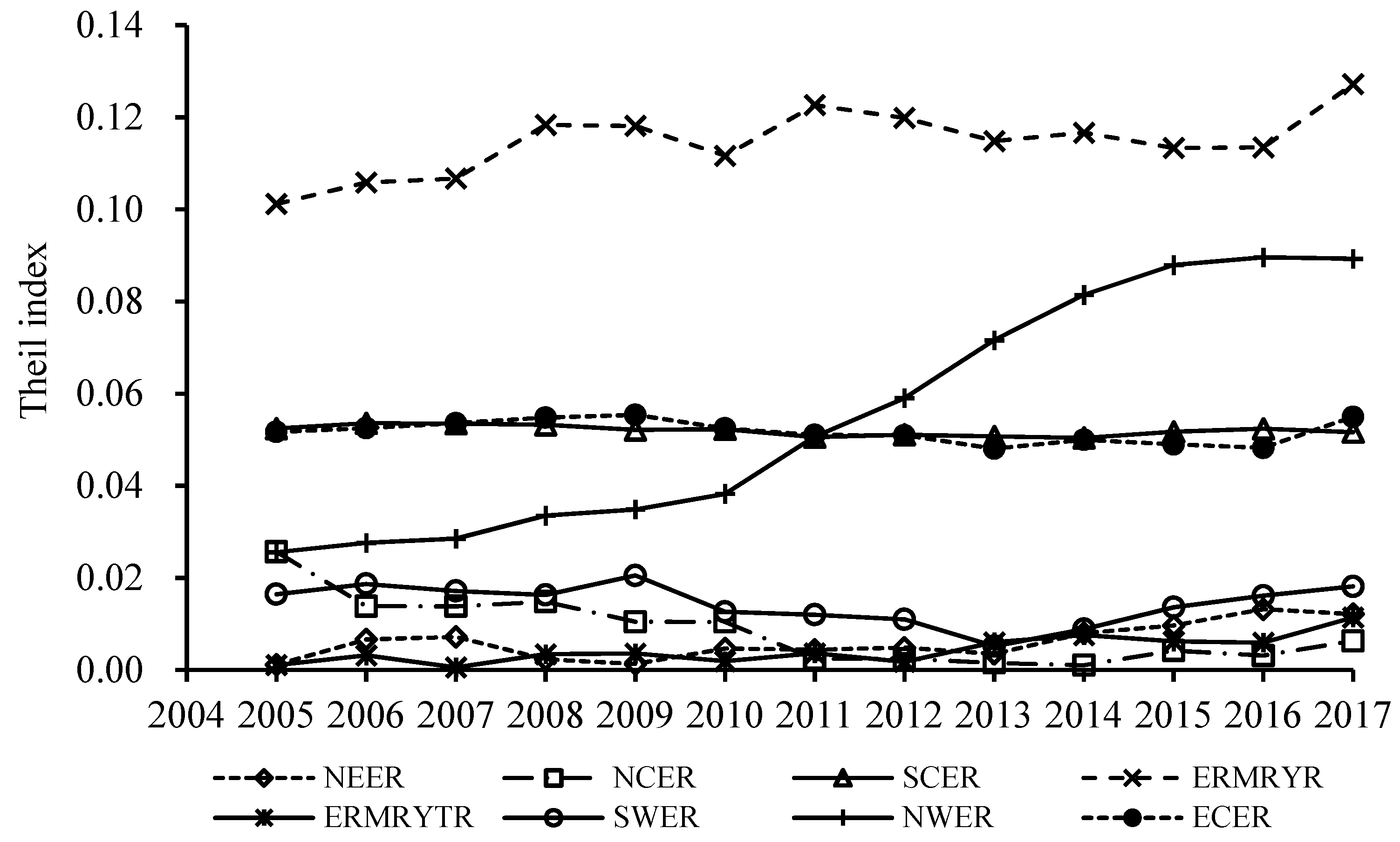
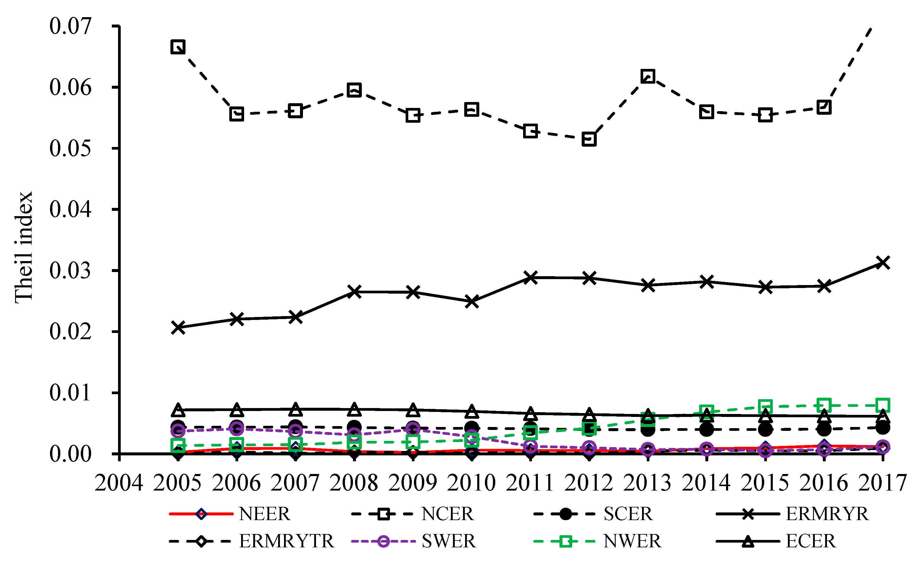
4.4. Regional Difference in Carbon Emissions and its Decomposition

During the study period, the overall difference acquired from the Theil index and the relevant results of emissions decomposition in China regions were showed in Figure 2. From Figure 2, the total Theil index (overall difference) of carbon emissions in the eight major economic regions exhibited a fluctuating ascending trend of “rising-falling-rising,” ranging from 0.37 to 0.48 during 2005–2017. That is to say, the total Theil index rose slowly in 2005–2008, and then declined slightly from 2008 to 2010, finally continued to increase in 2010–2017, with a mean annual growth rate of 3.21%. This implied that the overall difference in carbon emissions at the regional level remained a strong expansion tendency. As for the reasons, it may be associated with the increasing differences of regional economic growth, industrial structure, and policy orientation, along with the imbalanced energy production and consumption during the study period.

From the perspective of the source of the overall difference, the inter-regional difference in carbon emissions varied from 0.275 in 2005 to 0.371 in 2017, which was far higher than the corresponding intra-regional differences. However, this was contrary to the results obtained by Yang and Liu [14], who observed that the intra-regional difference of carbon emissions was far greater than the inter-regional differences. That may be attributed to the too large research unit, because Zhao’s research was based on the three regions of East, middle and West China. Moreover, the variation trend of inter-regional difference was almost similar to that of the overall difference from 2005 to 2017 (Figure 2). This result indicated that the overall difference was mainly caused by the inter-regional difference, which could be confirmed by the contributions of inter-regional and intra-regional differences. We found that the contribution of inter-regional differences showed a slightly increasing trend, whereas that of intra-regional inequality indicated a downtrend (

Table 2. Sources and contributions of carbon emission differences in China’s eight economic regions according to the Theil index in 2005–2017 (unit: %).

Year	NEER	NCER	ECER	SCER	ERMRYR	ERMRYTR	SWER	NWER	${\mathit{T}}_{\mathit{W}\mathit{B}\mathit{C}}$	${\mathit{T}}_{\mathit{W}\mathit{R}\mathit{C}}$
2005	0.42	9.33	18.79	19.04	36.76	0.39	5.98	9.29	72.55	27.45
	0.26	63.89	12.21	4.18	19.83	0.07	3.56	1.29
2006	2.36	4.92	18.62	19.00	37.54	1.13	6.63	9.80	74.60	25.40
	9.11	57.90	12.10	4.56	22.97	0.33	4.26	1.54
2007	2.56	4.92	19.07	19.03	37.96	0.21	6.11	10.14	74.47	25.53
	0.93	58.23	7.57	4.57	23.21	0.11	3.80	1.57
2008	0.79	5.00	18.46	17.94	39.86	1.16	5.49	11.30	74.20	25.80
	0.34	57.64	7.07	4.18	25.67	0.26	3.00	1.83
2009	0.45	3.53	18.69	17.58	39.85	1.21	6.92	11.76	74.84	25.16
	0.24	55.57	7.23	4.42	26.55	0.24	4.01	1.96
2010	1.64	3.68	18.45	18.39	39.27	0.68	4.45	13.45	74.34	25.66
	0.61	57.4	7.09	4.27	25.41	0.10	2.86	2.26
2011	1.48	0.80	17.17	17.00	41.24	1.23	4.04	17.05	75.24	24.76
	0.58	53.96	6.75	4.21	29.47	0.27	1.27	3.51
2012	1.61	0.82	16.93	16.97	39.80	0.60	3.65	19.61	75.73	24.27
	0.58	53.35	6.69	4.12	29.83	0.06	1.04	4.34
2013	1.17	0.51	15.94	16.82	38.08	2.00	1.72	23.75	73.85	26.15
	0.38	57.86	5.86	3.72	28.84	0.42	0.67	5.25
2014	2.47	0.32	15.43	15.55	36.00	2.34	2.73	25.14	75.79	24.21
	0.81	54.08	6.11	3.86	27.23	0.59	0.73	6.60
2015	2.88	1.26	14.59	15.41	33.76	1.85	4.06	25.78	76.58	23.42
	0.95	54.00	6.09	3.89	26.58	0.50	0.48	7.51
2016	3.86	0.92	14.10	15.31	33.16	1.74	4.72	25.89	76.55	23.45
	1.25	54.09	5.92	3.85	26.20	0.48	0.67	7.55
2017	3.28	1.70	14.81	13.92	34.27	3.07	4.89	24.06	77.20	22.80
	1.24	76.04	6.41	4.50	32.61	0.96	1.17	8.25

Note: The acronyms for regions are explained in Table 1. The underlined data is the contribution of the inter-regional difference of each economic region to the total inter-regional difference of the eight regions. The data without underline represents the contribution of intra-regional difference between provinces to the total intra-regional difference. T_WBC denotes the contribution of total inter-regional difference to the total difference of China’s carbon emissions. T_WRC represents the contribution of total intra-regional difference to the total difference of China’s carbon emissions.

). For instance, the contribution rates of inter-regional differences to the overall difference based on the Theil index were 72.55% in 2005 and 77.20% in 2017. The contribution rate of intra-regional difference to the overall difference in 2005 was 27.45%, falling to 22.80% in 2017. This showed that the contribution of inter-regional difference only had a slight increase during the research period, but future policy making and implementation should consider balancing inter-regional differences in carbon emissions.

For the inter-regional difference, it appeared that the Theil index was distinctly different, and showed the differentiation trend for various regions. As demonstrated in Figure 3, during the entire study period (2005–2017), the ERMRYR had the largest Theil index with a mean value of 0.115, followed by the NWER, SCER, and ECER, while the ERMRYTR showed the smallest inter-regional difference based on the Theil index, with a mean of 0.004. Except for an obvious uptrend of Theil index in the ERMRYR and NWER, other economic regions only presented marginal fluctuations in Theil index. These results demonstrated that the ERMRYR was the largest contributor in total inter-regional differences increase, followed by the NWER, SCER and ECER (Table 2). Compared with the inter-regional difference, the intra-regional difference based on the Theil index remained basically unchanged except for a slight rise (Figure 2), but the intra-regional difference in various economic regions showed a trend of differentiation in 2005–2017. From Figure 4, it is obvious that the NCER had the largest intra-regional difference with an average of 0.058 and a frequent fluctuation, followed by the ERMRYR, whose intra-regional difference witnessed a fluctuating upward trend, with a mean value of 0.025; while the other six economic regions only showed smaller intra-regional difference indexes, all of which were less than 0.01. This indicated that the NCER and ERMRYR were the largest two contributors in total intra-regional difference increase. However, the contribution of total intra-regional difference to the overall difference of carbon emissions was relatively small (Table 2).

From the perspective of contribution rate (Table 2), the contributions of total inter-regional difference to the overall difference in China’s carbon emissions were more than 72.50% in all years (2005–2017) and experienced an uptrend in this period, which indicating that carbon emissions between economic regions displayed significant divergence features. In China’s eight economic regions, the ones with a large contribution of inter-regional difference to the total inter-regional difference were the ERMRYR, the SCER, the ECER, and the NWER. The four regions jointly contributed to over 83.87% of the total inter-regional difference every year and showed a trend of fluctuation in the study period. Among them, the contribution of inter-regional difference of the NWER kept a continuous rising trend, which was in line with the change of inter-regional difference in the NWER described in Figure 3. With regard to the contribution of intra-regional difference, despite not being as large as that of inter-regional difference and exhibiting a gradual downward trend (the contribution rate decreased from 27.45% in 2005 to 22.80% in 2017, with an average of 24.93%, which showed that the carbon emission within the region was converging), there were also obvious discrepancies in the contribution of intra-regional (inter-provincial) difference to the total intra-regional difference across regions. As illustrated in Table 2, the top contributor to the total intra-regional difference appeared in the NCER, in which the contribution had a clear fluctuation, and increased sharply since 2016, with an average value of 58.0% between 2005 and 2017. It was closely followed by the ERMRYR, in which the intra-regional difference caused more than 19.83% contributions in 2005–2017, with a fluctuating upward trend, indicating that intra-regional differences between provinces in the ERMRYR were gradually broadening during the study period. Conversely, the ERMRYTR had the lowest contribution to total intra-regional difference, with an average of 0.337%, being far below all the regional average of 12.80%. Also, the intra-regional contributions of the remaining five economic regions were at medium levels and fluctuated between 0.263% and 8.255%, representing the average level of most regions.

From the above analysis, we can conclude that the inter-regional differences in carbon emissions and the internal differences in some regions such as the NCER and the ERMRYR were the main reasons for the overall difference in carbon emissions of China’s eight main economic regions during the study period, which also means that China’s carbon emission is not only different between regions, but also there is a gap that cannot be ignored between provinces within the region.

4.5. Influencing Factors of Regional Differences in China’s Carbon Emissions

The above results showed that there was an obvious spatial imbalance of carbon emissions in China’s eight major economic regions. In order to reveal the reasons for the regional differences in carbon emissions, we adopted the PLS-VIP method to explore the influences of various factors on carbon emissions in different economic regions. Considering whether it is necessary to use PLS-VIP method for regression analysis, a collinearity diagnosis on the influencing factors (i.e., explanatory variables) was first performed before using the PLS-VIP analysis. The diagnostic result confirmed that there was strong collinearity among explanatory variables because the values by a variance inflation factor (VIF) of explanatory variables (except the energy structure) were all greater than 10 (

Table 3. Variance inflation factor (VIF) values of influencing factors of carbon emission in NEER.

Explanatory Variable	lnP	lnA	(lnA)2	lnT	lnE	lnS	lnU
VIF	124.96	356.834	1643.34	26.30	6.11	74.86	1320.75

Note: Confined to the length of the thesis, Table 3 only listed the collinearity results of the influencing factors of carbon emissions in the NEER.

). According to the method described in Section 3.3, the interpretative test and the cross-validity test were used to determine the final cumulative explanatory ability of the principal components extracted from the factors affecting carbon emissions to the explanatory variables X and the response variable Y, as well as the cumulative cross-validity values of the principal components. As exhibited in

Table 4. Interpretation and cross-validation test of principal components base on partial least square (PLS) regression for carbon emissions and influencing factors in China’s eight economic regions.

Economic Region	Comp No.	R2X	R2X(cum)	R2Y	R2Y(cum)	Q2	Q2(cum)	α
NEER	Comp 1	0.684	0.684	0.894	0.894	0.814	0.814	0.05
	Comp 2	0.171	0.855	0.047	0.941	0.131	0.839	0.05
NCER	Comp 1	0.969	0.969	0.840	0.840	0.781	0.781	0.05
	Comp 2	0.006	0.975	0.154	0.994	0.304	0.847	0.05
SCER	Comp 1	0.786	0.786	0.787	0.787	0.672	0.672	0.05
	Comp 2	0.144	0.930	0.100	0.887	0.177	0.730	0.05
	Comp 3	0.063	0.994	0.096	0.983	0.839	0.956	0.05
ERMRYR	Comp 1	0.818	0.818	0.845	0.845	0.770	0.770	0.05
	Comp 2	0.123	0.941	0.069	0.914	0.209	0.818	0.05
ERMRYTR	Comp 1	0.830	0.830	0.877	0.877	0.831	0.831	0.05
	Comp 2	0.140	0.970	0.076	0.954	0.544	0.923	0.05
SWER	Comp 1	0.704	0.704	0.677	0.677	0.475	0.475	0.05
	Comp 2	0.207	0.911	0.174	0.852	0.364	0.666	0.05
	Comp 3	0.069	0.981	0.091	0.943	0.554	0.851	0.05
NWER	Comp 1	0.657	0.657	0.921	0.921	0.896	0.896	0.05
	Comp 2	0.164	0.821	0.071	0.991	0.767	0.976	0.05
ECER	Comp 1	0.963	0.963	0.877	0.877	0.845	0.845	0.05
	Comp 2	0.029	0.992	0.099	0.976	0.680	0.950	0.05

Note: The acronyms for regions are explained in Table 1. Comp No. indicates the number of principal components; R2x represents the variance contribution of the ith principal component extracted from the explanatory variables to the explanatory variable X, R²X(cum) denotes the cumulative variance contribution of the top i principal components extracted from the explanatory variables to the explanatory variable X; R²Y indicates the variance contribution of the ith principal component extracted from the explanatory variables to the dependent variable Y, R²Y(cum) indicates the cumulative variance contribution of the top i principal components extracted from the explanatory variables to the dependent variable Y; Q² means the cross validity of the principal component, Q²(cum) means the cumulative cross validity of the principal components; α is significant at the 0.05 level.

, in each economic region, the cumulative variance contribution rate of the principal components to the explanatory variables was more than 0.820, the cumulative variance contribution rate to the dependent variables was above 0.914, and the cumulative cross-validity was greater than 0.818. These results showed that it was reasonable to further use the PLS method to perform regression analysis based on the econometric model for carbon emissions.

Table 5. Elasticity coefficients of explanatory variables affecting carbon emissions in China’s eight regions.

Economic Region	Explanatory Variable
	lnP	lnA	(lnA)2	lnT	lnU	lnS	lnE
NEER	0.257	0.410	0.369	1.317	0.583	0.022	−0.112
NCER	0.809	0.762	0.008	0.791	0.456	0.751	−0.437
SCER	0.607	0.392	0.263	0.447	0.382	0.272	0.212
ERMRYR	0.346	0.226	0.197	−0.120	0.348	0.077	−0.117
ERMRYTR	0.310	0.310	0.259	−0.018	0.324	0.384	0.293
SWER	0.352	0.536	0.550	0.132	0.523	0.109	0.938
NWER	0.262	0.295	0.220	0.131	0.265	0.014	−0.196
ECER	0.798	0.596	0.375	0.526	−0.015	0.368	0.202
Average value	0.493(1)	0.441(2)	0.280(6)	0.401*(3)	0.363(4)	0.250(7)	0.310*(5)

Note: *Represents the average value calculated after taking the absolute value for the negative coefficient in the same variable, and the number in brackets is the ranking in all factors. The acronyms for regions are explained in Table 1.

and

Table 6. Variable importance of projection (VIP) value and ranking of the explanatory variable for carbon emissions in economic regions of China.

Economic Region	Explanatory Variable
	lnP	lnA	(lnA)2	lnU	lnT	lnS	lnE
NEER	1.018(5)	1.203(1)	1.164(2)	1.146(3)	1.065(4)	0.617(6)	0.581(7)
NCER	1.004(2)	1.002(3)	0.948(6)	0.974(5)	1.143(1)	0.989(4)	0.928(7)
SCER	1.128(1)	1.078(2)	1.032(4)	1.074(3)	0.982(5)	0.863(6)	0.799(7)
ERMRYR	1.056(3)	1.085(2)	1.009(4)	1.133(1)	0.962(5)	0.836(6)	0.760(7)
ERMRYTR	1.001(3)	1.078(1)	0.989(5)	1.072(2)	0.992(4)	0.947(7)	0.953(6)
SWER	1.309(1)	1.044(2)	0.878(6)	1.007(3)	0.816(7)	0.890(5)	0.993(4)
NWER	1.229(3)	1.253(1)	1.181(4)	1.230(2)	0.539(6)	0.815(5)	0.241(7)
ECER	1.142(1)	0.984(3)	0.956(6)	1.020(2)	0.968(5)	0.903(7)	0.969(4)
Average value	1.111(1)	1.091(2)	1.020(4)	1.082(3)	0.936(5)	0.855(6)	0.803(7)

Note: The number in brackets is the ranking in all factors. The acronyms for regions are explained in Table 1.

were respectively the regression results and the explanation abilities of various influencing factors on carbon emissions based on PLS-VIP method in each economic region. From the perspective of average value, among all the explanatory variables, the population size had the greatest impact on carbon emission, followed by the energy intensity, economic development level (the square term of GDP per capita was included in the economic development factor), urbanization, energy structure and industrial structure, which was different from the importance ranking of each factor’s average explanatory power (i.e., VIP value) for carbon emissions in the eight regions (Table 5 and Table 6). In terms of population, the population size of the eight economic regions was positively correlated with carbon emissions, with the elasticity coefficients ranging from 0.257 to 0.809 and an average of 0.493. The VIP values of the population size in all regions were above 1.0. This result indicated that population size had significantly positive effects on emissions growth and a strong ability to explain carbon emissions. It also suggested that the difference in population size was the main factor causing the difference in carbon emissions between regions. From Table 5, the regions with large population-scale effect on carbon emission increase were mainly the NCER, ECER, and SCER. Their elastic coefficients were 0.809, 0.798, and 0.607, respectively. The reasons for this may include the following two aspects: First, these regions have developed economy and superior geographical location [57]. Second, there are three municipalities directly under the central government—Beijing, Shanghai, and Tianjin in the NCER and ECER. Due to these reasons, the above regions attracted a large number of surplus labors from other regions, which led to the continuous increase in population of these three regions. For example, based on our calculation, from 2005 to 2017, the annual average growth rate of population in the NCER, ECER, and SCER were 1.24%, 1.10%, and 1.49%, respectively. As a result, with the improvement of residents’ living standards, the impact of population-scale in these three regions on carbon emission increase was inevitably greater than that of the other regions in our study. This further confirmed Deng et al.’s conclusion that population-size effect had a great impact on carbon emissions in such regions including municipalities directly under the central government [37]. Therefore, to control the population in the above regions and eliminate the uneconomical phenomenon of carbon emission caused by population-scale will play an important role in promoting carbon emission reduction. Furthermore, due to the influences of western development and the rise of central China, the population in the SWER, ERMRYR, and ERMRYTR obviously moved inward, which led carbon emissions to also have a certain population-scale effect. However, in the NEER and NWER, because there was no large internal migration in population [25], the population size effect was relatively weak compared to that in the above three regions (Table 5).

For the impact of economic development on carbon emissions, the elastic coefficients of GDP per capital in the eight economic regions were all positive, with a range of 0.226 to 0.762, and the average ranked the second among all factors, indicating that economic growth was the major factor to promote regional emissions increase during the study period. Specifically, the positive effect of GDP per capital on carbon emissions was the largest in the NCER and ECER, followed by that in the SWER, NEER, SCER, ERMRYTR, and NWER, while the per capital GDP in the ERMRYR showed the smallest positive effect in emissions increase (Table 5). This meant that economic development levels resulted from different development conditions (e.g., location difference, resources endowment and policy support, etc.) were distinctly various in different regions, and thus had different impacts on regional carbon emissions. From the perspective of the VIP value, the explanatory ability of GDP per capital in the eight major regions varied from 0.984 to 1.253, with an average of 1.091, ranking second in all the factors (Table 6). It showed that economic development had a strong ability to explain carbon emissions in all regions. Among them, in the NWER, the economic development had the strongest ability to explain carbon emission, indicating that it played a decisive role in the increase of carbon emissions in this region. Nevertheless, the weakest interpretability occurred in the ECER, in which the VIP value was 0.984. The reason may be that the ECER belongs to developed regions. With the enhancement of emission reduction awareness and the promotion of emission reduction technologies, the ability of economic development to explain carbon emissions was gradually weakened. Comprehensive considering the elasticity coefficient and explanatory capacity of per capital GDP to carbon emission, we can conclude that economic growth was the second driver for the differences in regional carbon emission, which was similar to the results reported by some previous researchers [14,19]. They found that per capital GDP was an important factor affecting the difference of carbon emission levels in East, Central, and West China. It is interesting to note that the square term of GDP per capital had a relatively weak effect on regional carbon emission (excluding the SWER), but most of its elastic coefficients were more than 0.25 (Table 5), and the VIP value was mostly close to or more than 1.0 (Table 6). On the one hand, it illustrated that the square term of GDP per capital could not be ignored in the interpretation of carbon emissions [58]. On the other hand, it also showed that no inverted U-shaped relationship appeared between economic development and carbon emissions in this period (2005–2017). Therefore, with the rapid economic development, the peak (or inflection point) of regional carbon emissions has not come. It is worth mentioning that, although the coefficients of the square term of per capital GDP were positive in all regions, the NCER coefficient almost approached to 0 (Table 5). This means that when the economic development reaches a certain level, it is possible to restrain emissions growth by improving emission reduction technology, optimizing the industrial structure and enhancing environmental awareness of the government and residents. Simultaneously, it also shows that the peak of Kuznets curve between carbon emission and GDP per capita will appear in the NCER in advance.

As far as the industrial structure was concerned, although the average of the elastic coefficients of the ratio of the second industry to GDP was the smallest, it was all positive in each economic region, which was consistent with the expectation that the increase of the proportion of the second industry will promote the growth of carbon emissions. However, from Table 5, the effect of industrial structure on energy-related carbon emission was quite different in various economic regions, and the elastic coefficients changed from 0.014 to 0.751, indicating that the industrial structure was also the contributor to regional carbon emission difference. The regions with great influence of industrial structure on carbon emission in order were the NCER, ERMRYTR, and ECER, and the VIP values of industrial structure in the NCER and ERMRYTR were close to 1.0, indicating that the industrial structure still had a strong ability to explain carbon emission in these two regions. It also means to further optimize the industrial structure and reduce the proportion of the secondary industry in the above regions, which is conducive to carbon emission mitigation. The regions with less impact of industrial structure on carbon emissions were the NWER and NEER, with the elastic coefficients of 0.014 and 0.022, respectively, and the VIP value of the NEER was less than 0.8 (Table 6), showing that the positive effect of industrial structure on carbon emissions was weak in these two regions. The results above also further indicated that the carbon emissions in the NCER and ERMRYTR were more easily affected by the industrial structure than those in the NWER and NEER, which may be related to the dependence of regional economic growth on the pull of the secondary industry [27]. For the developed NCER and ERMRYTR, although the industrial allocation has improved and the energy consumption of GDP has constantly reduced, the industrial structure is still relatively traditional. In addition, economic growth relies mainly on the energy-consuming secondary industry with high input-output efficiency. As the carbon emission of the secondary industry is far greater than that of the first and third industries, the regional carbon emission was related closely with the proportion of the secondary industry. This can be verified by the changing trend of the output proportion of the secondary industry to the GDP in the ERMRYTR (Figure 5). As for the share of secondary industry’s output in the GDP of the NCER, there was a significant downward trend. That may be caused by the decline of the proportion of the secondary industry in the Beijing-Tianjin area due to industrial structure optimization and upgrading and “capital function relief” (since 2014, the coordinated development of Beijing-Tianjin-Hebei region has become a national strategy, the industries with energy-intensive consumption and high pollution were shut down or transferred to the surrounding areas, and the proportion of secondary industry in Beijing decreased to 19.0% in 2017), which partially counteracted the influence of the large proportion of the secondary industry in Shandong and Hebei provinces and caused a significantly decline in the share of the output value of the secondary industry in the whole NCER. However, this does not mean that the carbon emission in the NCER was not significantly affected by the share of the secondary industry. The reason is that in the NCER, Shandong and Hebei are resource-intensive provinces. The economic development impelled the pillar industries such as chemical, metallurgy, building materials, machinery and automobile to consume large amounts of high-carbon fossil energy and produce a lot of carbon emissions, causing the elastic coefficient of the share of the secondary industry affecting carbon emissions reached 0.751 in this region (Table 5). This indicated that the development of the secondary industry in the NCER has reached a stage of serious diseconomy. Taking Shandong Province in the NCER as an example, its GDP increased from 1836.7 billion yuan in 2005 to 6300.2 billion yuan in 2017 (ranking the third in China), with an annual average growth of 24.3%, but its economic development was dominated by the secondary industry at the expense of energy resources. According to our calculation, the output value of the secondary industry accounted for over 52.0% of the provincial GDP during 2005–2017, which resulted in a large number of high carbon energy consumption, and thus carbon emissions. For example, the carbon emissions caused by coal consumption increased from 580 million tons in 2005 to 910 million tons in 2017, with an average annual growth of 5.2%. The NEER and NWER belong to underdeveloped areas. Although the proportion of resource-based cities and industries is relatively high, the industrial structure adjustment is vulnerable to the impact of macroeconomic policies. As a result, the proportion of the secondary industry output in total GDP changed in an “M” pattern (Figure 5). Moreover, the NWER had undertaken a large number of industries from the developed eastern region, which ultimately restrained the carbon emissions increase to a certain degree, resulting in a weak positive impact of the secondary industry’s share on the regional carbon emissions (Table 5, Table 6). This shows that the moderate transfer of the secondary industry to these regions may reduce national total carbon emissions.

In terms of urbanization, the average value of the urbanization elasticity coefficient of the eight regions was 0.363, ranking the fourth in all factors. This factor exerted positive effects on carbon emissions in most regions except the ECER where the negative effect appeared (Table 5). This result was not consistent with those of previous studies. Previous research showed that the urbanization had a positive role in promoting carbon emissions in the eastern region, no significant impact on carbon emissions in the central region, while had a negative impact in the western region [59]. In addition to the impact of time span (the sample data spanned the period from 1980 to 2014 in previous research), another reason for this phenomenon might be related to the large difference in study area division. In our study, the most significant effect of urbanization on carbon emissions occurred in the NEER, in which for every 1.0% increase in urbanization level, carbon emissions increased by about 0.583%. With regard to the VIP values of urbanization at the regional level, the ones of all economic regions except NCER were above 1.0 (Table 6), which showed that urbanization had an important explanatory capacity for carbon emissions of all regions in China [60]. Especially in the ERMRYR, the ability of the urbanization level to explain carbon emissions ranked the first among all the factors in the region, indicating that the urbanization played a decisive role in carbon emissions increase in the region. The reason may be that some provinces in the ERMRYR are in the early stage of industrialization and urbanization. Especially with the implementation of the strategies of western development and central rise, the focus of national investment and urbanization growth began to shift from the eastern coast to the central and western hinterland, which accelerated the extensive urbanization process in the ERMRYR, and increased the proportion of the urban population, so as to stimulate the consumptions of high-carbon energy and materials such as coal, cement and steel while promoting the infrastructure construction, consumer demand, and quality of life. Thus, the above reason ultimately brought more carbon emissions in the region. As regards the negative effect of the urbanization on carbon emission in the ECER, it may be related to three reasons. First, the ECER has entered the stage of new urbanization and high-quality development. The infrastructure construction has been basically completed, and the urban form has gradually changed to a compact type. Generally, the compact cities are conducive to reducing the demand for high-carbon fossil energy [20]. Second, the ECER promotes urbanization by the market allocation of resources and economic development. Therefore, with the rise of urbanization rate, the degree of industrial capital concentration will continue to improve, and then through scientific and technological innovation to improve the efficiency of energy utilization, leading to the gradual weakening of the positive effect of urbanization on carbon emissions, thereby cutting down carbon emissions. Third, the focus of national economic development and urbanization began to shift from the coastal to the inland provinces, and the speed of urbanization in the ECER slowed down. While exploring the new urbanization path, more attention was paid to economic transformation and upgrading, so as to promote the expansion of high energy consumption industries in the region to the central, western and the northeast regions, and thus inhibiting carbon emissions. Therefore, in the course of urbanization, the only way to reduce carbon emissions in the eight economic regions is to carry out new low-carbon urbanization.

Energy intensity played an active role in carbon emissions increase in most economic regions, but its elasticity coefficient and VIP value fluctuated greatly among the regions. The elasticity coefficient ranged from –0.120 to 1.317, with an average value of 0.401 (Table 5), and the VIP values varied from 0.539 to 1.143, with the average of 0.936 (Table 6), which indicated that the impact of energy intensity on the differences in regional carbon emission could not be ignored. To be specific, energy intensity played the most promoting role in carbon emissions increase in the NEER and NCER. For every 1% increase in energy intensity, the carbon emissions of the two regions increased by 1.317% and 0.791%, correspondingly, and their VIP values were as high as 1.065 and 1.143, respectively, indicating that energy intensity had a strong ability to explain carbon emissions. The reason was that in the research period, the industrial structure of the NEER and NCER (excluding the Beijing-Tianjin region) was relatively traditional, and there were more extensive resource-dependent enterprises. Additionally, in 2005–2006, with the improvement of the domestic investment environment and the acceleration of investment growth, the rise of absolute output inevitably brought more energy input (i.e., the increase of energy consumption intensity), causing carbon emissions growth. Hence, improving the efficiency of energy utilization is an important way to carbon emissions reduction in these regions. Contrarily, the positive effects of energy intensity in the ECER and SCER were relatively weak, and their VIP values were less than 1.0, indicating that energy intensity had no significant effect on carbon emissions. The main reason was that the industrial restructuring in such regions has been basically completed, and the overall level of energy efficiency has been improved. Besides, the demand for energy-consuming products due to economic development was close to saturation, and the public awareness of emission reduction was enhanced. The two reasons led to the decrease in carbon emissions, thus a weak positive effect of energy intensity. What was interesting was the energy intensity had the least positive effects on carbon emission in the NWER and SWER, while the negative effects were found in the ERMRYR and ERMRYTR (Table 5). Except that the VIP value of energy intensity in the NWER was less than 0.8, those in the other three regions were all in the range of 0.8–1.0 (Table 6). It was apparent that the energy intensity had a certain ability to explain carbon emission in the SWER, ERMRYR, and ERMRYTR. As for the above four regions, the reason why the energy intensity showed the smallest promoting or negative effects on carbon emissions, maybe that these economic regions are located in the central and western regions, and resource-dependent and high-energy consumption enterprises accounted for a large proportion in secondary industry, which was vulnerable to the impact of national macroeconomic policies (Since 2005, China has implemented energy-saving and emission-reduction policies for key industries, resulting in a significant reduction of energy consumption per unit product). Therefore, the adjustment of industrial structure or technological progress has great elasticity to restrain carbon emissions. Besides, these regions undertook some high-tech industries from the eastern developed areas, and eliminated some local backward production enterprises, causing the enhancement of energy efficiency and the corresponding reduction of carbon emissions [61].

As shown in Table 5, the energy structure represented positive and negative effects in the eight economic regions. On the whole, the average value of elasticity coefficients of energy structure was small and ranked behind in all factors, but the elasticity coefficients fluctuated greatly among the regions, with the range of −0.437 to 0.938, indicating that the energy structure was also an important factor causing the difference in regional carbon emissions. Among the eight economic regions, the absolute value of the energy structure effect in the SWER and NCER was larger than that in other economic regions (Table 5). Specifically, the energy structure effect of the NCER was significantly negative, and the VIP value was close to 1.0 (Table 6). On the one hand, it showed that the energy structure was important to the change of carbon emissions in this region; on the other hand, with the increase in the proportion of new energy use, the energy diversification effect in the region was increasingly obvious, and the energy structure is becoming more reasonable. For example, the Beijing-Tianjin area, located in the NCER, is rich in clean energy resources. In recent years, with the advantages in economy, science-technology, and education, as well as good external environment, Beijing and Tianjin have vigorously developed a new energy industry and formed a green energy industry cluster with the wind, solar, biomass, lithium batteries, and geothermal energy as the main body. In 2017, the ratio of coal, oil, natural gas and other energy sources was adjusted to 27.6:22.1:1.7:48.6 in the Beijing-Tianjin area. Although the coal consumption of Shandong Province, located in the NCER, has always been dominated (In the past 13 years, the average coal consumption ratio of this province was 72%, which was greater than the national average of 70%), the proportion of raw coal in total energy consumption of the whole region decreased from 65% in 2005 to 49% in 2017. As coal (including its products) is the energy with the largest carbon emission coefficient, the higher the share of coal in primary energy consumption, the more carbon emissions (Every 1% increase in coal proportion may increase carbon emissions by about 0.053%). Thus, the improvement of energy structure can effectively inhibit the growth of carbon emissions and shows a negative driving effect on carbon emissions. As regards the significantly positive effect of energy structure in the SWER, the reasons may include the following three aspects. First, it was related to the economic underdevelopment and the inelastic demand of energy (especially coal) for economic growth of the SWER. Second, the region is China’s main energy-produced base, and the energy consumption structure dominated by coal has not been changed for a long time. Third, the promotion and application of carbon emission reduction technology could not keep up with the increasing speed of energy consumption, especially coal. The above reasons resulted in a strong positive impact of energy structure on carbon emissions. In addition, the VIP value of energy structure in the SWER reached 0.993 (Table 6), indicating that the energy structure dominated by coal is one of the important factors to promote carbon emissions increase in the region. In the developed ECER, SCER, and ERMRYTR, economic development needs to consume a large amount of energy as the driving force. Although there are large-scale energy inputs from outside the regions (such as West–East electricity transmission, North–South coal transportation, and West–East gas transmission), the impact of energy consumption structure on carbon emissions is greatly affected by energy policies and macroeconomic situation. Especially in 2007–2010, owing to the influence of the financial crisis, alternative energy sources in the above-mentioned regions were used again, coupled with the slowdown in new energy investment, leading to a weak positive effect of energy structure on carbon emissions (Table 5). However, the VIP values of the energy structure in the ECER and ERMRYTR were all close to 1.0 (Table 6), indicating that the energy structure had a good explanation ability for carbon emissions of these two regions. Additionally, Table 5 showed that the energy structure effects in the NEER, ERMRYR, and NWER were negative, and the VIP values were all below 0.8 (Table 6). This demonstrated that the impact of the energy structure in these three regions was not important. As for the negative correlation between energy structure and carbon emissions, it may because the NEER, ERMRYR, and NWER are important coal-oil production bases in China, and fossil energy accounts for over 90% of the total energy resources. Although the industries of these regions are relatively backward, the coal-fired power industry is relatively developed. When the inhibition effect of coal treatment technology is greater than the promoting effect of coal proportion increase on carbon emission, the carbon emissions will gradually reduce (namely negative effect).

5. Conclusions and Policy Proposals

Based on Theil index and PLS-VIP method, this study makes a quantitative analysis on regional differences and causes of carbon emissions in China’s eight major economic regions from 2005 to 2017, as well as the impact degree of various factors on carbon emissions in different regions. The main conclusions are as follows:

(1) In the study period, the carbon emissions of each economic region in China witnessed a rigid increase trend and showed a phased feature. The carbon emission and its annual average growth rate were significantly different across regions. The top three emitters were the ERMRYR, NCER, and ECER, and the growth rate of carbon emissions in the NWER was significantly higher than that in other regions.

(2) From 2005 to 2017, the overall difference in carbon emissions of the eight major economic regions showed a fluctuating and increasing trend, which was mainly caused by the expansion of the inter-regional difference. The contribution of total inter-regional difference to the overall difference in carbon emissions was more than 72.5% yearly and indicated an upward trend with the time. Nevertheless, the contribution of the inter-regional difference of each region to total inter-regional difference displayed a trend of differentiation. The contribution of total intra-regional difference to the overall difference of carbon emissions in the eight economic regions was relatively small, and the intra-regional difference of each region was also at different levels.

(3) The influence degree and explanatory ability of various factors on regional carbon emissions and regional emissions discrepancy were quite different. Population size, economic development, and energy intensity were the three prominent factors affecting regional carbon emission changes and regional emissions differences, their elastic coefficients and VIP values for carbon emissions changed obviously in the eight regions. Industrial structure and urbanization displayed positive impacts on regional emissions but with significant differences. The most impacts of carbon emissions by industrial structure and urbanization occurred in the NCER and NEER, respectively, while the weak effects appeared in the NEER and ECER. The influence of energy structure on regional carbon emission and its explanatory power was weak on the whole, but the elastic coefficients and VIP values changed distinctly in different regions, indicating that the impact of energy structure on regional carbon emission difference could not be ignored.

According to the research results, several policy suggestions are put forward for regional emissions reduction in China. First, as the changing trends of carbon emissions and their influence factors were different in various regions, each region should formulate emission mitigation policies in the light of its own emission characteristics and key influencing factors. Second, the regions with large-scale carbon emissions or fast-growing carbon emissions should be regarded as the foremost regions of national emission reductions. Finally, considering the continuous growths of energy demand, strengthening emissions reduction in the energy industry, promoting renewable energy generation and tightening up demand-side management is the key to achieve emission reduction goals in most regions of China. More specifically,

(1) As the major carbon emission regions, the NCER, ECER, and ERMRYR should strictly control the total carbon emissions and take greater responsibility for carbon reductions in China. In the NCER, in addition to keeping the upper limit of population and paying attention to the uneconomical effect of carbon emission caused by population scale, the large industrial provinces, such as Shandong and Hebei, should actively connect with enterprises in Beijing-Tianjin area, carry out technical cooperation in the energy industry, and promote emission reduction by the low-carbon oriented industrial restructuring and energy structure optimization. Concerning the ECER, in which industrialization and urbanization have already entered the latter stage, more efforts are needed to release the emissions mitigation potential of high-end manufacturing industry, commercial service industry, and urban residential consumption. The ERMRYR should make use of its resource advantages to improve emission reduction space by enhancing energy utilization efficiency, innovating energy (such as coal and oil) management methods and extending industrial chain.

(2) The NWER and SWER are the main energy-exporting regions, in which energy intensity was relatively high and carbon performance was low, the energy industry played a leading role in regional emissions growth. Hence, in formulating the emission reduction targets of these two regions, we should take effective control of energy intensity and improve the carbon emission performance of the energy industry as the primary task. Moreover, for the NWER, with the fastest growth of carbon emission, it is imperative to reduce the share of the heavy chemical industry and optimize the regional energy structure. For the SWER, which focuses on the development of tourism, we should push on the energy conservation and emission mitigation of the tourism industry chain.

(3) With regard to the SCER, ERMRYTR, and NEER, as they are industrializing and urbanizing, their carbon emissions displayed an uptrend. We should moderately reduce the total carbon emissions and control the level of carbon intensity in these three regions. More concretely, less developed NEER should continue to implement the Northeast Revival Strategy and realize regional emission reduction through the transformation and upgrading of resource-based industries, the introduction of a large number of advanced production technologies and controlling the pace of urbanization process. In the ERMRYTR, we should vigorously develop renewable energies (such as hydropower and biogas) and increase the proportion of high-tech industries in this region to appropriately control carbon intensity and promote the low-carbon-oriented economy. The SCER was large energy-importing region, in which foreign investment, high-quality talents and labor resources have obvious advantages. However, commercial services and household consumption may play important roles in influencing carbon emissions of this region. Therefore, the SCER should pay more attention to reducing the emissions of the service industry and residential consumption and take the aforesaid advantages to expand services in energy saving and emissions reduction and develop the modern service industry. Besides, the development of nuclear energy and wind power should be the focus to improve the energy structure.

It should be pointed out that there are still some limitations in this research. First, we only analyzed the impacts of economic growth, population size, energy intensity, energy structure, and industrial structure, as well as the level of urbanization on regional carbon emissions, without in-depth study of other factors, such as technological progress, foreign direct investment, and residential energy consumption on carbon emissions. Although energy intensity can reflect technological progress to some extent, other variables may also be important factors affecting carbon emissions. Second, when discussing the impact of economic development on carbon emissions, some major economic events on economic growth were not taken into account; and major economic events are often important factors affecting carbon emissions. Third, the selection of different conversion coefficients has a certain influence on the accurate calculation of energy consumption. However, in this study, the energy consumption based on standard coal was calculated according to the conversion coefficient in China Energy Statistics Yearbooks, which does not necessarily reflect the most realistic situation. Therefore, it is of great significance to strengthen the experimental study of energy conversion standard coefficient and further improve the level of coal treatment technology for revealing the relationship between energy consumption and carbon emission, as well as driving carbon emission reduction. These issues will be considered in our future research.

References

1. Tao, S.; Li, B.G.; Gasser, T.; Ciais, P.; Piao, S.L.; Balkanski, Y.; Hauglustaine, D.; Boisier, J.P.; Chen, Z.; Huang, M.T. The contribution of China’s emissions to global climate forcing. Nature 2016, 531, 357–361. [Google Scholar]
2. Ye, B.; Jiang, J.J.; Sheng, L.C. Quantification and driving force analysis of provincial-level carbon emissions in China. Appl. Energy 2017, 198, 223–238. [Google Scholar] [CrossRef]
3. National Development and Reform Commission of China (NDRC). Enhanced Actions on Climate Change: China’s Intended Nationally Determined Contributions; National Development and Reform Commission of China: Beijing, China, 2015. (In Chinese)
4. Lai, L.; Huang, X.J.; Yang, H.; Julian, R.T. Carbon emissions from land-use change and management in China between 1990 and 2010. Sci. Adv. 2016, 2, e1601063. [Google Scholar] [CrossRef] [PubMed] [Green Version]
5. Li, K.; Lin, B.Q. Economic growth model, structural transformation, and green productivity in China. Appl. Energy 2017, 187, 489–500. [Google Scholar] [CrossRef]
6. Liu, Z.; Guan, D.B.; Moore, S.; Lee, H.; Su, J.; Zhang, Q. Climate policy: Steps to China’s carbon peak. Nature 2015, 522, 279–281. [Google Scholar] [CrossRef] [Green Version]
7. Shan, Y.L.; Liu, J.H.; Liu, Z.; Xu, X.H.; Shao, S.; Wang, P.; Guan, D.B. New provincial CO2 emission inventories in China based on apparent energy consumption data and updated emission factors. Appl. Energy 2016, 184, 742–750. [Google Scholar] [CrossRef] [Green Version]
8. Wang, J.; Yang, J. Regional carbon emission intensity disparities in China based on the decomposition method of Shapley value. Resour. Sci. 2014, 36, 557–566. (In Chinese) [Google Scholar]
9. Chen, J.D.; Xu, C.; Cui, L.B.; Huang, S. Driving factors of CO2 emissions and inequality characteristics in China: A combined decomposition approach. Energy Econ. 2019, 78, 589–597. [Google Scholar] [CrossRef]
10. Clarke-Sather, A.; Qu, J.S.; Wang, Q.; Zeng, J.J.; Li, Y. Carbon inequality at the sub-national scale: A case study of provincial-level inequality in CO2 emissions in China 1997–2007. Energy Policy 2011, 9, 5420–5428. [Google Scholar] [CrossRef]
11. Yang, J.; Wang, J.; Zhang, Z.Y. Inter-provincial discrepancy and abatement target achievement in carbon emissions: A study on carbon Lorenz curve. Acta Sci. Circumstantiae 2012, 32, 2016–2023. (In Chinese) [Google Scholar]
12. Cheng, Y.Q.; Wang, Z.Y.; Ye, X.Y. Spatiotemporal dynamics of carbon intensity from energy consumption in China. J. Geogr. Sci. 2014, 24, 631–650. [Google Scholar] [CrossRef] [Green Version]
13. Liu, C.J.; Hu, W. Does foreign direct investment increase China’s carbon productivity? Empirical analysis based on the spatial panel Durbin model. World Econ. Stud. 2016, 1, 99–109. [Google Scholar]
14. Yang, J.; Liu, H.J. Regional difference decomposition and influence factors of China’s carbon dioxide emissions. J. Quant. Tech. Econ. 2012, 5, 36–49. (In Chinese) [Google Scholar]
15. Wang, F.; Wu, L.H.; Yang, C. Driving factors for growth of carbon dioxide emissions during economic development in China. Econ. Res. J. 2010, 2, 123–136. (In Chinese) [Google Scholar]
16. Wang, M.; Feng, C. Decomposition of energy-related CO2 emissions in China: An empirical analysis based on provincial panel data of three sectors. Appl. Energy 2017, 190, 772–787. [Google Scholar] [CrossRef]
17. Jiang, J.H. An evaluation and decomposition analysis of carbon emissions in China. Resour. Sci. 2011, 33, 597–604. (In Chinese) [Google Scholar]
18. Zha, D.; Zhou, D.; Zhou, P. Driving forces of residential CO2 emissions in urban and rural China: An index decomposition analysis. Energy Policy 2010, 38, 3377–3383. [Google Scholar]
19. Li, G.Z.; Li, Z.Z. Regional difference and influence factors of China’s carbon dioxide emissions. China Popul. Resour. Environ. 2010, 20, 22–27. (In Chinese) [Google Scholar]
20. Xiao, M.Y.; Fang, Y.L. The impact of FDI on carbon emissions in the eastern region of China: An empirical analysis based on STIRPAT model. J. Cent. Univ. Financ. Econ. 2013, 7, 59–64. (In Chinese) [Google Scholar]
21. Zhang, L.Q.; Li, R.F.; Chen, S.P.; Zu, Y.W.; Xu, X.W. Trend prediction and analysis of driving factors of carbon emissions from energy consumption during the period of 1995–2009 in Anhui province based on the STIRPAT model. Resour. Sci. 2012, 34, 316–327. (In Chinese) [Google Scholar]
22. Wang, Y.; Yang, G.; Dong, Y.; Cheng, Y.; Shang, P.P. The scale, structure and influencing factors of total carbon emissions from households in 30 provinces of China: Based on the extended STIRPAT model. Energy 2018, 11, 1125. [Google Scholar] [CrossRef] [Green Version]
23. Zhang, Y.; Zhang, L.Q.; Bao, T.T. Research on the influential factors of carbon emissions in the process of urbanization in Anhui province-based on STIRPAT model. Resour. Environ. Yangtze Basin 2014, 23, 512–517. (In Chinese) [Google Scholar]
24. Zhou, X.; Zhang, M.; Zhou, M. A comparative study on decoupling relationship and influence factors between China’s regional economic development and industrial energy–related carbon emissions. J. Clean. Prod. 2017, 142, 783–800. [Google Scholar] [CrossRef]
25. Jiang, J.; Ye, B.; Xie, D.; Tang, J. Provincial-level carbon emission drivers and emission reduction strategies in China: Combining multi-layer LMDI decomposition with hierarchical clustering. J. Clean. Prod. 2017, 169, 178–190. [Google Scholar] [CrossRef]
26. Shen, L.; Wu, Y.; Lou, Y.; Zeng, D.; Shuai, C.; Song, X. What drives the carbon emission in the Chinese cities?—A case of pilot low carbon city of Beijing. J. Clean. Prod. 2018, 174, 343–354. [Google Scholar] [CrossRef]
27. Liu, Z.X. Research on the relationship between energy consumption, economic growth and carbon emission in China. Coal Econ. Res. 2011, 4, 37–43. (In Chinese) [Google Scholar]
28. Geng, Y.H.; Tian, M.Z.; Zhu, Q.; Zhang, J.J.; Peng, C.H. Quantification of provincial-level carbon emissions from energy consumption in China. Renew. Sustain. Energy Rev. 2011, 15, 3658–3668. [Google Scholar] [CrossRef]
29. Ren, S.; Fu, X.; Chen, X.H. Regional variation of energy-related industrial CO2 emissions mitigation in China. China Econ. Rev. 2012, 4, 1134–1145. [Google Scholar] [CrossRef]
30. Liu, Z.; Geng, Y.; Lindner, S.; Guan, D. Uncovering China’s greenhouse gas emission from regional and sectoral perspectives. Energy 2012, 45, 1059–1068. [Google Scholar] [CrossRef] [Green Version]
31. Zhou, X.; Zhou, M.; Zhang, M. Contrastive analyses of the influence factors of interprovincial carbon emission induced by industry energy in China. Nat. Hazards 2016, 81, 1405–1433. [Google Scholar] [CrossRef]
32. Zhang, X.F.; Han, X.; Zhang, Q.C. Regional difference and influence factors of carbon emissions: Empirical analysis based on partial least squares method. J. Ind. Technol. Econ. 2013, 7, 100–109. (In Chinese) [Google Scholar]
33. Liu, Y.; Chen, Z.M.; Xiao, H.; Yang, W.; Liu, D.H.; Chen, B. Driving factors of carbon dioxide emissions in China: An empirical study using 2006–2010 provincial data. Front. Earth Sci. 2017, 11, 156–161. [Google Scholar] [CrossRef]
34. Wang, H.; Chen, C.C.; Pan, T.; Liu, C.L.; Chen, L.; Sun, L. County scale characteristics of CO2 Emission’s spatial-temporal evolution in the Beijing-Tianjin-Hebei Metropolitan region. Environ. Sci. 2014, 35, 385–393. (In Chinese) [Google Scholar]
35. Chen, Z.M.; Wu, S.M.; Ma, W.B. Driving forces of carbon dioxide emission for China’s cities: Empirical analysis based on extended STIRPAT Model. China Popul. Resour. Environ. 2018, 28, 45–54. (In Chinese) [Google Scholar]
36. Sun, Y.H.; Zhong, W.Z.; Qing, D.R. Analysis on differences of carbon emission intensity of each province in China based on Theil index. Financ. Trade Res. 2012, 3, 1–7. (In Chinese) [Google Scholar]
37. Deng, J.X.; Liu, X.; Wang, Z. Characteristics analysis and factor decomposition based on the regional difference changes in China’s CO2 emission. J. Nat. Resour. 2014, 29, 189–200. (In Chinese) [Google Scholar]
38. Liu, H.G.; Fan, X.M. CO2 emissions transfer embedded in inter-regional trade in China. Acta Ecol. Sin. 2014, 343, 3016–3024. (In Chinese) [Google Scholar]
39. Kang, Y.Q.; Zhao, T.; Yang, Y.Y. Environmental Kuznets curve for CO2 emissions in China: A spatial panel data approach. Ecol. Indic. 2016, 63, 231–239. [Google Scholar] [CrossRef]
40. O’Mahony, T. Decomposition of Ireland´s carbon emissions from 1990 to 2010: An extended Kaya identity. Energy Policy 2013, 59, 573–581. [Google Scholar]
41. Sun, W.; He, Y.; Chang, H. Regional characteristics of CO2 emissions from China’s power generation: Affinity propagation and refined Laspeyres decomposition. Int. J. Glob. Warm. 2017, 11, 38–66. [Google Scholar] [CrossRef]
42. Mi, Z.; Zhang, Y.; Guan, D.; Shan, Y.; Liu, Z.; Cong, R.; Yuan, X.C.; Wei, Y.M. Consumption-based emission accounting for Chinese cities. Appl. Energy 2016, 184, 1073–1081. [Google Scholar] [CrossRef] [Green Version]
43. Goh, T.; Ang, B.W. Tracking economy-wide energy efficiency using LMDI: Approach and practices. Energy Effic. 2019, 12, 829–847. [Google Scholar] [CrossRef]
44. Wang, H.; Ang, B.W.; Su, B. Assessing drivers of economy-wide energy use and emissions: IDA versus SDA. Energy Policy 2017, 107, 585–599. [Google Scholar] [CrossRef]
45. Wang, Q.; Wang, Y.; Zhou, P.; Wei, H. Whole process decomposition of energy related SO2 in Jiangsu Province, China. Appl. Energy 2017, 194, 679–687. [Google Scholar] [CrossRef]
46. Wang, Z.; Yang, L. Delinking indicators on regional industry development and carbon emissions: Beijing-Tianjin-Hebei economic band case. Ecol. Indic. 2015, 48, 41–48. [Google Scholar] [CrossRef]
47. Wang, S.; Fang, C.; Guan, X.; Pang, B.; Ma, H. Urbanization, energy consumption, and carbon dioxide emissions in China: A panel data analysis of China’s provinces. Appl. Energy 2014, 136, 738–749. [Google Scholar] [CrossRef]
48. Wang, H.; Zhou, P. Assessing global CO2 emission inequality from consumption perspective: An index decomposition analysis. Ecol. Econ. 2018, 154, 257–271. [Google Scholar] [CrossRef]
49. Ramakrishnan, R. A multi-factor efficiency perspective to the relationships among world GDP, energy consumption and carbon sioxide emissions. Technol. Forecast. Soc. Chang. 2006, 73, 483–494. [Google Scholar]
50. Wold, H. Soft modeling by latent variables: The non-linear iterative partial least squares (NIPALS) approach. J. Appl. Probab. 1975, 12, 117–142. [Google Scholar] [CrossRef]
51. Chong, I.G.; Jun, C.H. Performance of some variable selection methods when multicollinearity is present. Chemom. Intell. Lab. Syst. 2005, 78, 103–112. [Google Scholar] [CrossRef]
52. Development Research Center of the State Council. Regional Policy and Coordinated Development 1995; Development Research Center of China State Council: Beijing, China, 1995. (In Chinese)
53. IPCC. Intergovernmental Panel on Climate Change Guidelines for National Greenhouse Gas Inventories: Volume 2 Energy. Available online: http://www.ipcc-nggip.iges.or.jp/public/2006gl/vol2.html (accessed on 12 July 2018).
54. National Bureau of Statistics of China (NBSC). Chinese Energy Statistics Yearbook; NBSC, Beijing, China Statistics, 2006–2018; NBSC: Beijing, China, 2006–2018. (In Chinese)
55. National Bureau of Statistics of China (NBSC). Chinese Statistics Yearbook; NBSC, Beijing, China Statistics, 2006–2018; NBSC: Beijing, China, 2006–2018. (In Chinese)
56. Guan, D.; Meng, J.; Reiner, D.M.; Zhang, N.; Shan, Y.L.; Mi, Z.F.; Shao, S.; Liu, Z. Structural decline in China’s CO2 emissions through transitions in industry and energy systems. Nat. Geosci. 2018, 11, 551–555. [Google Scholar] [CrossRef]
57. Zhang, H.G.; Wang, C.J.; Wang, F. Examining the driving factors of energy related carbon emissions using the extended STIRPAT model based on IPAT identity in Xinjiang. Renew. Sustain. Energy Rev. 2017, 67, 51–61. [Google Scholar]
58. Peng, J.M.; Wu, R.H. Decomposition of Pearl River Delta’s carbon emissions based on LMDI method. China Popul. Resour. Environ. 2012, 22, 69–74. (In Chinese) [Google Scholar]
59. Chen, W.H.; Lei, Y.L. Analysis of the impact path on factors of China’s energy-related CO2 emissions: a path analysis with latent variables. Environ. Sci. Pollut. Res. 2017, 24, 5757–5772. [Google Scholar] [CrossRef]
60. Wu, H.; Gu, S.Z.; Guan, X.L. Analysis on relationship between carbon emissions from fossil energy consumption and economic growth in China. J. Nat. Resour. 2013, 28, 381–390. (In Chinese) [Google Scholar]
61. Liu, X.Z.; Gao, C.C.; Zhang, Y. Spatial dependence pattern of carbon emission intensity in China’s provinces and spatial heterogeneity of its influencing factors. Sci. Geogr. Sin. 2018, 38, 681–690. (In Chinese) [Google Scholar]
Figure 1. Changes in carbon emissions of China’s eight major economic regions in 2005–2017. Note: Table 1.
Sustainability 12 02576 g001
Figure 2. Decomposition results of China’s regional carbon emissions from 2005 to 2017.
Sustainability 12 02576 g002
Figure 3. Inter-regional differences in carbon emissions of China’s eight economic regions according to Theil index between 2005 and 2017. Note: The acronyms for regions are explained in Table 1.
Sustainability 12 02576 g003
Figure 4. Intra-regional differences in carbon emissions of China’s eight economic regions according to Theil index between 2005 and 2017. Note: The acronyms for regions are explained in Table 1.
Sustainability 12 02576 g004
Figure 5. The proportion of secondary industry output in the GDP of some economic regions. Note: The acronyms for regions are explained in Table 1.
Sustainability 12 02576 g005