Mapping Maize Fields by Using Multi-Temporal Sentinel-1A and Sentinel-2A Images in Makarfi, Northern Nigeria, Africa

Abstract

A timely and accurate crop type mapping is very significant, and a prerequisite for agricultural regions and ensuring global food security. The combination of remotely sensed optical and radar datasets presents an opportunity for acquiring crop information at relative spatial resolution and temporal resolution adequately to capture the growth profiles of various crop species. In this paper, we employed Sentinel-1A (S-1) and Sentinel-2A (S-2) data acquired between the end of June and early September 2016, on a semi-arid area in northern Nigeria. A different set of (VV and VH) SAR and optical (SI and SB) images, illustrating crop phenological development stage, were employed as inputs to the two machines learning Random Forest (RF) and Support Vector Machine (SVM) algorithms to automatically map maize fields. Significant increases in overall classification were shown when the multi-temporal spectral indices (SI) and spectral band (SB) datasets were added with the different integration of SAR datasets (i.e., VV and VH). The best overall accuracy (OA) for maize (96.93%) was derived by using RF classification algorithms with SI-SB-SAR datasets, although the SI datasets for RF and SB datasets for SVM also produced high overall maize classification accuracies, of 97.04% and 97.44%. The outcomes indicate the robustness of the RF or SVM methods to produce high-resolution maps of maize for subsequent application from agronomists, policy planners, and the government, because such information is lacking in our study area.

1. Introduction

Recent global food insecurity has been largely observed in Latin America and Africa, mainly associated with a range of factors, including an increase in the human population, armed conflicts, climate change, and inequality in accessing sufficient and quality food [1]. For example, countries with a large population in the African sub-continent have suffered food insecurity, which is largely connected to agricultural production [2]. Nigeria is the largest and most populous country in Africa, with over 200 million people as of 2019 [3], and it has seen rapid population growth coupled with armed conflicts and thus an increase in food insecurity. Nigeria has already witnessed famine in recent years, which was largely associated with the agricultural sector. Agricultural sectors in countries like Nigeria and other countries in Africa have a crucial role in the nation’s food security and sustainable development. Maize is one of the staple foods in Africa [4] and Nigeria [5] and the demand is skyrocketing with an increase in population. The area cultivated with maize in a year/season provides an early indication of the potential production and possible warning for food shortage and famine. Consequently, there is an urgent need to develop a famine early warning framework through mapping and monitoring maize production areas to ensure food security and sustainable development in countries like Nigeria.

Timely and accurate estimation of agricultural production area under a certain crop like maize at regional and global scales provides a means to assist government decision-makers and planners [6]. The Earth Observation (EO) system offers an incredible direction and promotes scientists and policymakers to move beyond conventional agricultural surveying techniques in quantifying the area under a crop and tackle associated agrarian problems [7,8]. With the increased availability of current and historical remotely sensed imagery archives, it is now possible to monitor farmlands in a timely, cost-effective, and repetitive way [9,10]. For example, data from Moderate Resolution Imaging Spectroradiometer (MODIS) and Landsat satellite images have been widely used for agricultural mapping and monitoring [11,12].

One of the major problems with the application of remotely sensed imagery, particularly optical imagery in tropical countries like Nigeria, is weather conditions, including clouds and rain, affecting the quality of images [13]. This problem could largely limit the mapping and classification of a cropped area, such as fields under maize [14]. Synthetic Aperture Radar (SAR) imagery shows potential as it is not affected by weather and clouds [15,16,17,18]. The integrated use of optical and SAR data offers a great opportunity for mapping the cropped area [17,19]. For example, Blaes et al. [20] reported a 5% increase in accuracy by adding ERS and RADARSAT imagery with optical SPOT and Landsat images. Lamin R. Mansaray et al. [21] successfully used five Sentinel 1A and one Landsat-8 images for paddy rice field mapping in urban Shanghai and reported a 5% increase in overall accuracy than individuals. Rosenthal and Blanchard [22] and Brisco et al. [23] also reported that the combination of optical and radar datasets in crop mapping increased the overall accuracy by 20% and 25%, respectively. Other studies revealed an increased percentage range of 5% and 8% when the two data sources were employed [24,25]. Zhou et al. [26] utilized Sentinel-1A and Landsat-8 in mapping winter wheat in the urban agricultural region in China.

Recently, a growing number of studies utilizing Sentinel-1 (S-1) and Sentinel-2 (S-2 images in agricultural research have been in focus [27,28,29]. This shows strong potential for both satellite sensors to be used by the remote sensing community and to develop a method that distinguishes various crops using remotely sensed data [27,30]. Thus, they provide unprecedented perspectives for monitoring vegetation dynamics and land use/cover. Several studies have demonstrated that optical multi-temporal satellite imagery allows crop type mapping over different climate and diverse cropping systems [30,31,32,33,34]. For example, recently, S-1 and S-2 were applied to assess the suitability of data for crop classification in Japan [35].

Choosing a suitable model for classification is essential for successful crop mapping. Several classification algorithms have been employed to conduct crop mapping, however, Random Forest (RF) and Support Vector Machine (SVM) are the two most commonly employed machine learning algorithms in remote sensing community for mapping purposes, because RF and SVM classifiers are two algorithms with high potential for classifying high-dimensional data [36,37]. Most of the researchers have studied either Sentinel-1 alone or Sentinel-2 alone for crop mapping [27,38]. Sonobe et al. [35] studied the suitability of data from Sentinel-1A and -2A for crop classification in order to improve the recognition accuracy of dryland crops. TerraSAR-X image and RapidEye optical data have also been used to identify the accuracy of maize using RF in Northwestern Benin, West Africa [39]. Additionally, COSMO-SkyMed (CSK) and Radarsat-2, an integration of remote sensing data in conjunction with optical data, were used to acquire accurate classification results for maize [40]. Unfortunately, in all the aforementioned studies, few studies have been conducted incorporating Sentinel-1 and Sentinel-2 multi-temporal images in maize mapping. The potential of maize mapping accuracies with the RF and SVM classification algorithms has rarely been reported with single and different combinations of S-1 and S-2 datasets, in rain-fed, heterogeneous, and fragmented agricultural land.

However, the integration of Sentinel sensor datasets for mapping maize field is scarce. Moreover, the success in mapping crops using the combined images to large extent depends on accurate differentiation between crop and other land covers. The small field size creates a major issue in this situation. For example, mapping cropped area under a smallholder farm system, such as maize fields in Nigeria, becomes very difficult. The use of multi-temporal satellite images from the beginning, middle, and end of cropping seasons could help tackle the problem, as crop growth stages will have distinct features and be different from other crops.

The goal of the present paper is to examine the potential of multi-temporal S-2 (optical), S-1 (SAR) multi-temporal satellite imagery, and their combinations for automatically mapping maize fields in Makarfi, Kaduna State, Nigeria. To achieve this, the following objectives are addressed in this study:

• To evaluate the integration of Sentinel-1A (SAR) and Sentinel-2A (optical) images for maize crop mapping using RF and SVM;
• To provide the optimal combination of S-1 dual-polarization channels that complement the S-2 for maize mapping;
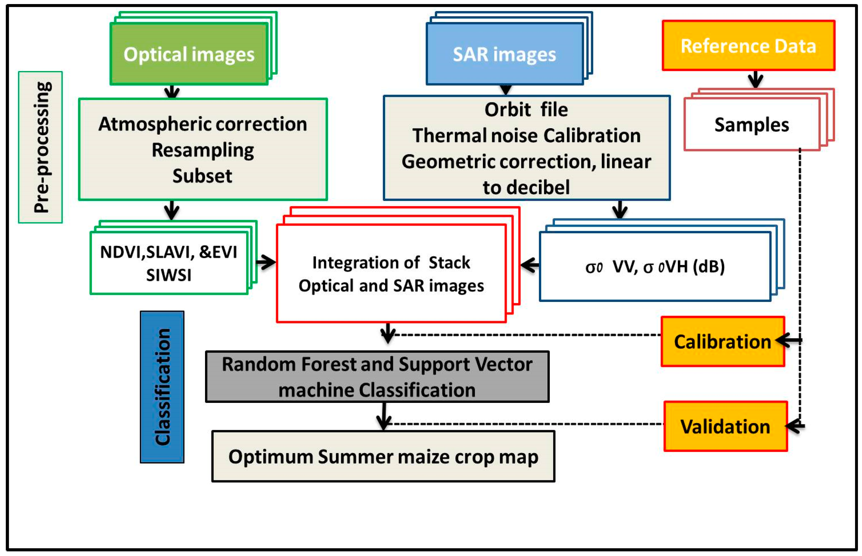
• To design a simple framework for integrating S-1 and S-2 images to map maize crops and use for agricultural applications.

2. Materials and Methods

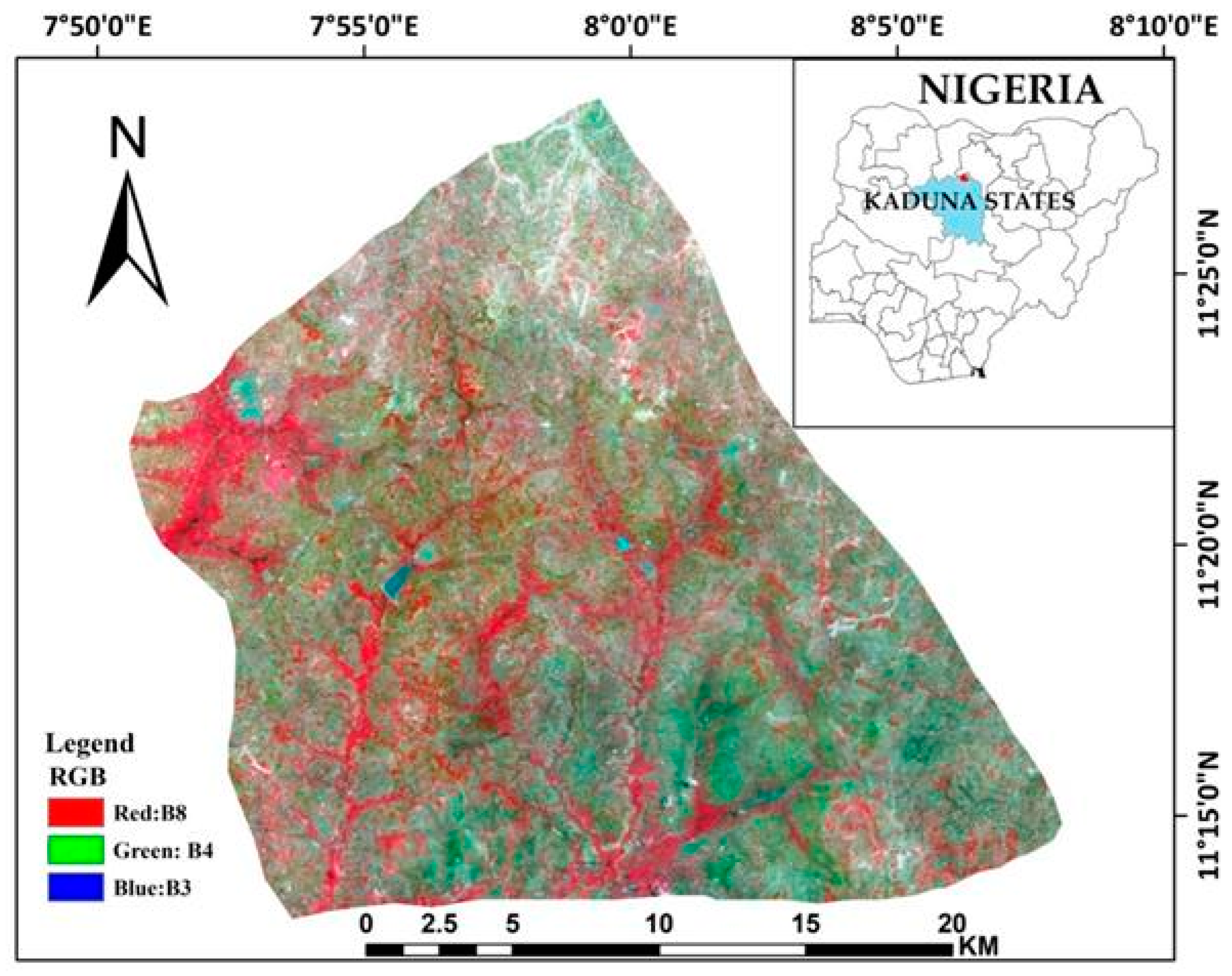
2.1. Study Area

Makarfi Local Government Area (central latitude 11°22’N and longitude 7°52’E) located in Kaduna State, Nigeria (Figure 1). Makarfi is one of the major maize growing areas of Kaduna State and has higher average productivity compared to other local government areas [41]. The main maize growing system in this county relies on smallholder farms, where most of the farm sizes are fragmented by various land cover types. The study area within the Northern Guinea savannah agro-ecological zone [42], is characterized by undulating plain with Cambisols and Acrisols dominated soil types. This region covers an area of about 541 km² with a tropical climate, based on the Köppen–Geiger system. The climate is suitable to support optimal conditions for growing maize. The average annual temperature ranges from 36 °C in the hot months of March through May to 12 °C in the cold months of July through September. The mean annual precipitation is 1016 mm. The monthly average rainfall is about 361 mm between May and September, with the wettest month being August.

According to the local agricultural calendar, the growing season of maize is from the end of May to the end of September. Nearly four months (June–September) of this period are considered the precipitation season with fewer numbers of cloud-free days. This places a constraint on acquiring optical remotely sensed data. Therefore, this region can be an ideal representative of growing maize at a smallholder scale in a tropical climate to examine the potential of dense multi-temporal SAR imagery in conjunction with a few optical data.

2.2. Field Data Collection

In Makarfi region, maize is planted at the end of May to early June and harvested in mid-September. We used official spatial data of maize planted region from the International Institute of Tropical Agriculture (IITA), Kano, Nigeria, for the period from 2014 to 2018. The main goal of this field campaign was to improve crop productivity and profitability for small-scale maize farmers in Africa (Ethiopia, Tanzania, and Nigeria). The data was collected by experienced agricultural officers along with the assistance of farmers in the regions. Noteworthy that any bias or considerations associated with this survey were not reported for subsequent procedures. In this study, we first extracted sample points related to the Makarfi region. We collected a substantial maize sample points (100) during the field campaign as our region of interest (ROI), these point were randomly acquired from the maize fields with the help of Global Positioning System (GPS) device, and recorded with a good accuracy. Besides maize sample points, we randomly acquired additional training and validation sample in combination with previous for the remaining five classes by visually interpreting the geo-referenced Google Earth images based on the ground truth. These classes were collected by supervised visual inspection and local knowledge of the region on Google Earth imagery. Based on the target crop (maize), the broad land cover classes in Makarfi in which a classification was designed, into six dominant Land Use/Land Covers classes, including maize fields, build-up, grassland, bare land, water bodies, and others were recognized. The build-up, grassland and bare land classes, later were dissolved to Others class, hence, we have three classes i.e. maize fields, water and others classes. These sample data of each class were separated randomly into two-third for training and one-third were preserving for validation, respectively. Regarding that the maize fields were our main target of the study, large training data depicting the maize class was derived for the image classification as adopted in Onojeghuo et al., [43].

2.3. Satellite Data and Pre-Processing

2.3.1. Sentinel-1 Image and Preprocessing

The European Space Agency (ESA) launched the Sentinel-1A (S-1A) satellite in April 2014. Sentinel-1A is the first of its series programs, as part of the Copernicus programs for the monitoring and observation of the Earth’s surface, and for the development of many operational applications for environmental monitoring. The Synthetic Aperture Radar (SAR) is carried out by two satellites (1A and 1B) and with a frequency of 5.4 GHz. The two satellites are indifferent to weather conditions and allow data acquisition day and night, the main features detected by Sentinel in the study area were single and dual-polarization images (VV and VH). In this study, we employed six C-band data (wavelength ~ 6 cm) in the form of Interferometric Wide (IW) swath images, acquired by the Sentinel-1 (S-1) satellite between June and early September 2016. S-1A images were acquired from the web site (https://scihub.copernicus.eu/dhus/#/home). The Ground Range Detected (GRD) products Level-1C images were used (

Table 1. A detailed description of S-1 and S-2 data acquisitions in 2016.

Sentinel-1 (SAR)		Sentinel-2 (Optical)
Azimuth Resolution	10	Band ID	Spatial Resolution—10/20/60 m
Polarization	Dual (VV-VH)	Band 1	(Coastal)—0.443 µm
		Band 2	(Blue)—0.490 µm
		Band 3	(Green)—0.560 µm
		Band 4	(Red)—0.665 µm
		Band 5	(Red Edge)—0.705 µm
Mode	IW	Band 6	(Red Edge)—0.740 µm
		Band 7	(Red Edge)—0.783 µm
		Band 8	(NIR)—0.842 µm
Incidence angle	Ascending 30.9–46	Band 8A	(NIR)—0.865 µm
		Band 9	(Water)—0.940 µm
		Band 10	(SWIR)—1.375 µm
		Band 11	(SWIR)—1.610 µm
		Band 12	(SWIR)—2.190 µm
Dates		Dates
29-Jun-16		22-Jun-16
11-Jul-16		23-Aug-16
23-Jul-16		11-Sep-16
4-Aug-16
16-Aug-16
9-Sep-16

).

In this study, six S-1 images of the study site were imaged at an incidence angle (0) of about 30.9–46 of the maize growing season in Makarfi. We performed several processing steps on a different image that was made up of an Orbit file, and then, we applied removal of thermal noise, followed by radiometric calibration, geometric correction, and finally speckle filtering [44], and then converted to sigma for the subsequent analysis.

2.3.2. Sentinel-2 Image and Preprocessing

Sentinel-2A (S-2A) is the second satellite launched by the (ESA) in June 2015. The S-2A has 13 spectral bands at different spatial resolutions (10, 20, 60 m). The S-2 characteristics are presented in Table 1. We retrieved three S-2 data from their open access hub, and the images were corrected atmospherically, using the Sentinel Applications Platform (SNAP) version 7.0 with the help of Sen2Cor 4, an atmospheric correction toolbox. We resampled bands with different spatial resolutions to 10 m using the nearest neighbor interpolation method [45]. This was employed to ensure that the pixel size of S-2 images corresponded with the identified maize field.

We derived four spectral indices from S-2 images. The Normalized Difference Vegetation Index (NDVI) was first proposed by Rouse et al. [46], and is the vegetation index most commonly employed in the remote sensing community, because it has the capability to map land covers and crops. Many studies have used the index and achieved great success [47]. The Enhanced Vegetation Index (EVI), Specific Leaf Area Vegetation Index (SLAVI), and finally, Shortwave Infrared Water Stress Index (SIWSI) are shown in

Table 2. Formulas of spectral indices features.

Spectral Indices	Formula	References
Normalized Difference Vegetation index	$NDVI=\frac{NIR-R^{*}}{NIR+R}$	[48]
Enhanced Vegetation Index	$EVI=2.5 \frac{pNIR-pR}{pNIR+6pR-7.5pB+1}$	[49,50]
Specific Leaf Area Vegetation Index	$SLAVI=\frac{NIR}{NIR+SWR2}$	[51]
Shortwave Infrared Water Stress Index	$SIWSI=\frac{NIRa-SWIR1}{NIR+SWR1}$	[52]

.

2.4. Classification Scheme

2.4.1. Feature Integration

We evaluated the effect of spectral bands, indices and SAR datasets used on the classification performances. The spectral indices were computed for each image, as presented in Table 2. SAR datasets were computed on S-1A, as shown in Table 1. These datasets were used alone or in association with the SAR images with a different date, i.e., 13 the spectral bands for S-2A and two polarized channels (VV and VH) for S-1A images. In essence, seven datasets were employed in this study, these were as follows:

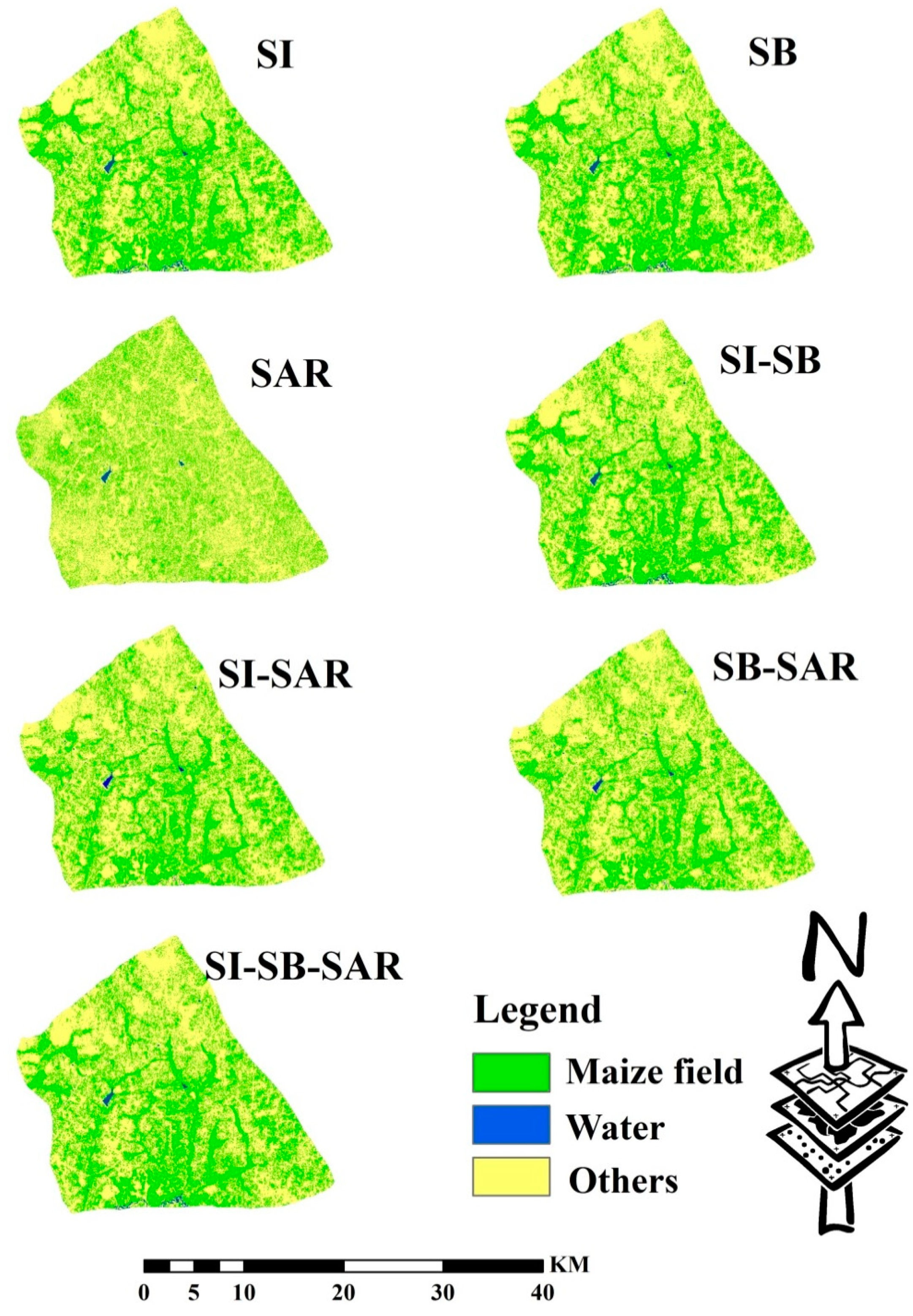
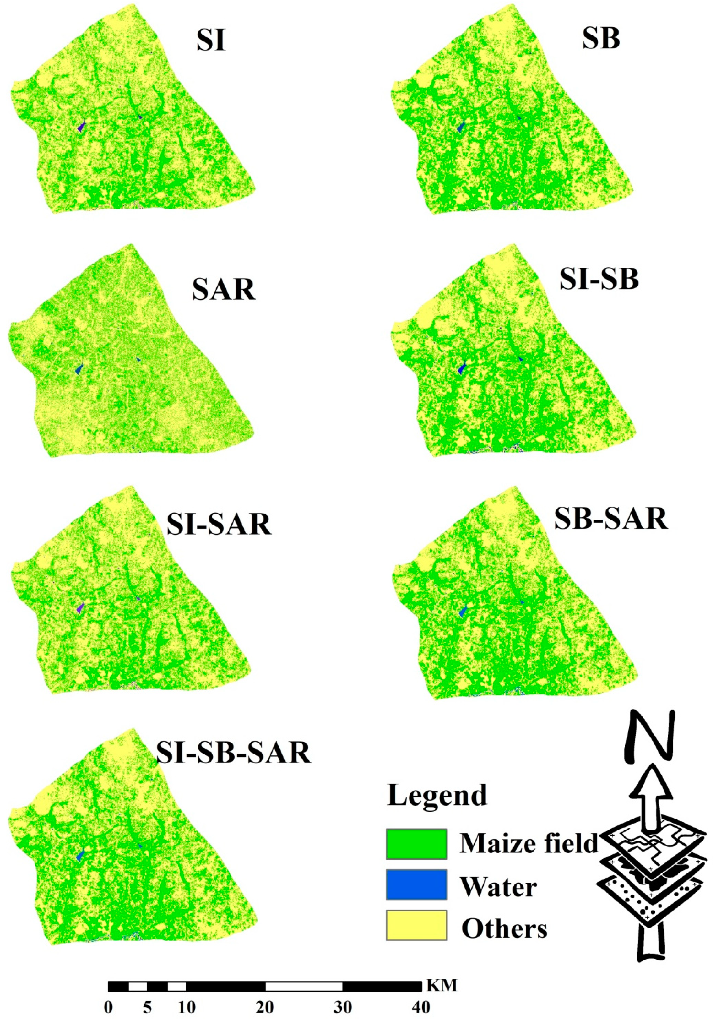
• Spectral indices only (SI);
• Spectral bands only (SB);
• Synthetic Aperture Radar (SAR);
• Spectral indices only and spectral bands only (SI-SB);
• Spectral indices only and Synthetic Aperture Radar (SI-SAR);
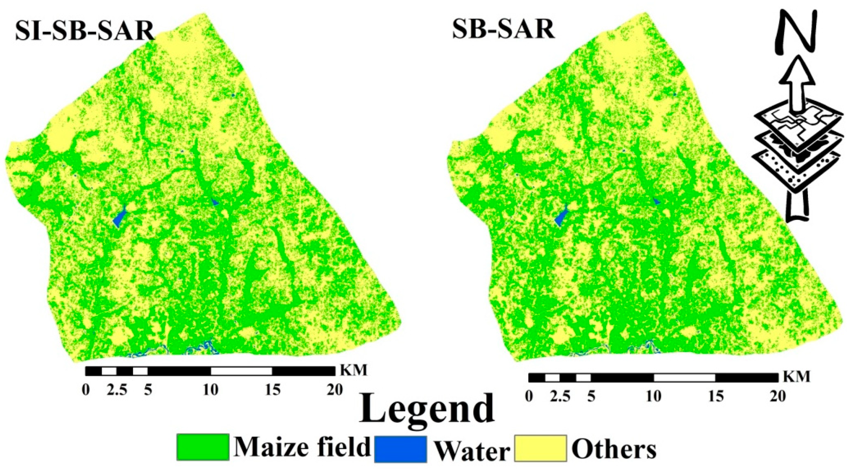
• Spectral bands only and Synthetic Aperture Radar (SB-SAR);
• Spectral indices, Spectral bands, and Synthetic Aperture Radar (SI-SB-SAR).

2.4.2. Classification Algorithms

Many classification techniques have been applied in the community of remote sensing for mapping over agricultural fields [53]. In this study, the two most known classification techniques were employed. The RF and SVM algorithms, which are supervised classification methods, were used to classify maize field and other classes during summer 2016.

The RF algorithm is an ensemble classifier that employs a set of classification and regression trees in order to make a prediction [54]. It was chosen over other classification models because it performs well on huge input datasets with several different features [55], and hence, it has been used by previous research for mapping purposes with tremendous success [51,56,57]. The two RF parameters are the number of trees (ntree), and the number of variables used for tree nodes splitting (mtry), which was created by randomly selecting samples from the training dataset [57]. We tuned the parameter randomly to determine the optimum one using the tune function. In this study, the optimal number of trees (ntree) was set between 150, 300, 500, and 1000, while the optimal mtry was set on the mtry vector factor with a default mtry being set as the square root of the total number of datasets. RF has the capability to detect the information that is valuable in each of its features, which is one of its strengths. RF classifiers possess the highest efficiency in terms of accuracy with limited processing time. We used the EnMAP-Box software, which is free, and an open source plug-in in QGIS capable of processing raster images.

The SVM algorithm is a machine learning that strives to maximize the margin between classes (the crops) through finding the optimal hyperplane in the n-dimensional classification space [36]. Several kernel functions have already been proposed, the one commonly employed is radial basis function (RBF) kernels [58]. In this study, an SVM with (RBF) kernel was employed. SVM strives to locate the decision boundaries which produce an optimal separation of classes [59]. The two parameters are the C regularization parameter for the kernel functions to be tuned. One important advantage of SVMs is their kernel function: by choosing a suitable kernel function, a complex problem could be solved. One weakness of the SVM is that of high cost in terms of computing time. The major parameters of SVM modeling include gamma and cost. In this study, the C parameter was set up between 150, 300, 500, and 1000, while the other parameter was set at default. We used ENVI software (Exelis Visual Information Solutions., Broomfield, CO, USA), version 5.3.

2.4.3. Accuracy Assessment

For all the classification schemes, the overall accuracy (OA), producer’s accuracy (PA), user’s accuracy (UA), and Cohen’s kappa coefficient of agreement (κ) were computed using the confusion matrices, with the aim to evaluate the accuracy of the produced crop maps [60]. Furthermore, McNemar’s test was adopted in this study, in order to evaluate the superiority of the two classifier methods. In other words, the test analyzed the significance of the difference between the classification derived from the six datasets. It is a non-parametric test, quite simple to understood and execute. Besides this, it is very precise and sensitive compared with other tests, such as the Kappa z-test. The analysis was based on a standard normal (χ²) statistics, which was computed from two error matrices using Equation (1):

$$x^2=\frac{\left(f_{12}-f_{21}\right)}{f_{12}+f_{21}},$$

(1)

where $f_{12}$ indicates the number of cases which were incorrectly classified by classifier one but correctly classified by classifier two, while $f_{21}$ implies the number of cases which were correctly classified by classifier one but incorrectly classified by classifier two.

An illustration of the methodological workflow adopted for this study is in the flow chart below (Figure 2).

3. Results—Support Vector Machines and Random Forests comparison

SVM and RF are the two most used machine learning methods, and their abilities to map crops and land cover using multi-source high spatial-resolution satellite images were compared. In this study, the evaluation was performed by using the seven datasets, explained in Section 2.4.1, consisting of maize and other cover classes.

3.1. SVM and RF Results

Table 3. The maize and land cover classes overall accuracy (OA) with producer’s accuracy (PA) and User’s accuracy (UA) obtained using RF and SVM.

RF								SVM
		SI		SI-SB		SI-SB-SAR		SI		SI-SB		SI-SB-SAR
		PA	UA	PA	UA	PA	UA	PA	UA	PA	UA	PA	UA
	Maize	95.38	92.99	94.82	95.68	94.65	94.41	95	95.4	92.43	95.7	93.19	94.78
	Water	77.55	99.13	91.16	100	88.11	100	70.07	100	88.44	100	86.01	100
150	Others	97.3	97.73	98.42	97.88	97.93	97.75	98.29	97.45	98.53	97.02	98.15	97.23
	OA	96.45		97.33		96.88		96.93		96.73		96.62
	Kappa	0.91		0.94		0.93		0.93		0.92		0.92
		PA	UA	PA	UA	PA	UA	PA	UA	PA	UA	PA	UA
	Maize	95.68	92.94	94.4	96.08	94.39	94.72	95.12	95.66	92.56	95.2	93.28	94.04
	Water	79.59	99.15	91.16	100	88.81	100	70.07	100	89.12	100	88.81	100
300	Others	97.26	97.89	98.56	97.72	98.5	97.68	98.38	97.5	98.34	97.08	97.85	97.3
	OA	96.54		97.32		96.92		97.04		96.63		96.47
	Kappa	0.92		0.94		0.93		0.93		0.92		0.91
		PA	UA	PA	UA	PA	UA	PA	UA	PA	UA	PA	UA
	Maize	95.34	93.07	94.65	95.88	94.65	94.37	95.12	95.37	92.56	95.2	93.49	93.49
	Water	78.91	100	91.84	100	88.81	100	70.07	100	89.12	100	88.81	100
500	Others	97.34	97.75	98.48	97.82	97.91	97.77	98.27	97.49	98.34	97.08	97.62	97.37
	OA	96.5		97.34		96.88		96.96		96.63		96.37
	Kappa	0.92		0.94		0.93		0.93		0.92		0.91
		PA	UA	PA	UA	PA	UA	PA	UA	PA	UA	PA	UA
	Maize	95.77	93.76	94.61	95.92	94.56	94.6	95.3	95.38	93.03	94.85	93.58	93.58
	Water	77.55	99.13	91.16	100	88.81	100	70.07	100	89.12	100	88.81	100
1000	Others	97.6	97.88	98.5	97.79	98.01	97.74	98.27	97.55	98.19	97.24	97.65	97.4
	OA	96.77		97.33		96.93		97		96.66		96.41
	Kappa	0.92		0.94		0.93		0.93		0.92		0.91

shows the averaged producer’s accuracy (PA) and user’s accuracy (UA) per class category, kappa and overall accuracy (OA) of SI (i.e., the lower case), SI-SB (the medium with the average number of features), and SI-SB-SAR (the higher with the vast amount of datasets) for SVM and RF.

In the lower case, the analysis of OA values indicated that SVM outperformed RF using the same feature datasets, with 300 C parameters for SVM and 1000 trees for RF. In the SI-SB case, the results of the OA percentage show that SVM underperformed RF using the same feature datasets, with 150 C parameters for SVM and 500 trees for RF. In the last case (SI-SB-SAR), the OA values show that SVM also underperformed RF using the same largest number of features, with 150 C parameters for SVM and 1000 trees for RF. Moreover, RF with SI-SB obtained good results. Furthermore, the OA differences between the RF and SVM were not always observed by looking at individual kappa values. Therefore, there was no much difference in kappa for SI-SB between SVM and RF, which would give rise to variation in OA.

With concern about the input datasets, SVM and RF had greater kappa differences among SI, SI-SB, and SI-SB-SAR. However, this was slightly higher for SI-SB. The RF classifier was more sensitive compared to SVM in terms of input feature sets. It could be observed that for differences per maize class and other land cover classes for “input features” the integration did not increase in any percentage. Despite the balanced training data, this is an agreement with the literature demonstrating that the RF classifier performs better [61], while sometimes SVM prevails [62]. Besides this, in all the classifiers, differences may also arise for the thematic land cover: RF is better on maize, others, and water, whereas SVM is suitable in all classes.

Several studies have employed the comparison between RF and SVM indicating their performances with different remote sensing data using both classifiers [63,64,65,66].

Table 4. McNemar test for the significant differences in RF and SVM classification.

S/N	Comparison	RF Z-score	SVM Z-score	SL 95%
1	SI versus SB	9.631	9.588	S
2	SI versus SAR	8.723	8.619	S
3	SI versus SI-SB	9.626	9.593	S
4	SI versus SI-SAR	9.560	9.570	S
5	SI versus SB-SAR	9.603	9.601	S
6	SI versus SI-SB-SAR	9.604	9.587	S
7	SB versus SAR	8.720	8.620	S
8	SB versus SI-SB	9.624	9.595	S
9	SB versus SI-SAR	9.558	9.572	S
10	SB versus SB-SAR	9.601	9.602	S
11	SB versus SI-SB-SAR	9.602	9.589	S
12	SAR versus SI-SB	9.689	9.662	S
13	SAR versus SI-SAR	9.623	9.639	S
14	SAR versus SB-SAR	9.666	9.670	S
15	SAR versus SI-SB-SAR	9.667	9.657	S
16	SI-SB versus SI-SAR	9.558	9.571	S
17	SI-SB versus SB-SAR	9.601	9.602	S
18	SI-SB versus SI-SB-SAR	9.602	9.589	S
19	SI-SAR versus SB-SAR	9.606	9.603	S
20	SI-SAR versus SI-SB-SAR	9.607	9.590	S
21	SB-SAR versus SI-SB-SAR	9.604	9.588	S

shows a slight improvement by the RF classifier; this could possibly be because of the ability of RF to deal with the high-dimensionality of the feature space.

3.2. Effect of Different Data Integration on the Maize Crop Mapping

The three datasets explained in the previous section were meant or designed to investigate the significant role of SI, SI-SB, and SI-SB-SAR at the end season crop mapping. SI datasets only use spectral indices, SI-SB combines the spectral indices and spectral band, and SI-SB-SAR includes SAR. These different three datasets were all used for RF and SVM classifiers. When only applying SI, 12 spectral indices were needed in order to get a maize map with high overall accuracy, since our main concern was maize, while the performance of SI for identifying the “water” and “others” class categories was relatively considered in this study. When using the combined SI-SB, (41 stacked features) from the images. It can also be observed that the performance of SI-SB slightly improved compared with SI only. We further integrated the SAR datasets; i.e., SI-SB-SAR: 12, 39, and 12 features were stacked. There was no improvement in the overall accuracy. The OA of SI and SI-SB-SAR were the same. Therefore, the inclusion of SAR datasets did not exhibit any increase as previous work reported [47].

3.3. Result of RF, SVM, and Accuracy Evaluation for SI, SI-SB, and SI-SB-SAR

With the RF classification, the integration of phenology information, that is, SI and SB, to the dual-polarized channels, the overall classification accuracy substantially increased. In this case, for spectral indices, spectral bands combined with SAR datasets, the OA increased from 80.60% (k = 0.50) to 96.2% with (k = 0.93), a difference of 16% increase was observed at 95% significant level, as indicated by McNemar test (Table 4). The overall accuracy of SI and SB did not increase (

Table 5. Error matrix of RF.

SI							SB
	Maize	Water	Others	Total	PA	UA		Maize	Water	Others	Total	PA	UA
Maize	2239	0	149	2388	95.77	93.76	Maize	2215	0	88	2303	94.74	96.18
Water	0	114	1	115	77.55	99.13	Water	0	135	0	135	91.84	100
Others	99	33	6101	6233	97.6	97.88	Others	123	12	6156	6291	98.59	97.85
Total	2338	147	6251	8736			Total	2338	147	6244	8729
SAR							SI-SB
	Maize	Water	Others	Total	PA	UA		Maize	Water	Others	Total	PA	UA
Maize	1326	5	516	847	56.76	71.79	Maize	2213	0	95	2308	94.65	95.88
Water	0	57	62	119	39.86	47.9	Water	0	135	0	135	91.84	100
Others	1010	81	5642	6733	90.71	83.8	Others	125	12	6156	6293	98.48	97.82
Total	2336	143	6220	8699			Total	2338	147	6251	8736
SI-SAR							SB-SAR
	Maize	Water	Others	Total	PA	UA		Maize	Water	Others	Total	PA	UA
Maize	2222	3	183	2408	95.12	92.28	Maize	2204	2	122	2328	94.35	94.67
Water	0	99	0	99	69.23	100	Water	0	128	0	128	89.51	100
Others	114	41	6037	6192	97.06	97.5	Others	132	13	6098	6243	98.04	97.68
Total	2336	143	6220	8699			Total	2336	143	6220	8699
			SI-SB-SAR
				Maize	Water	Others	Total	PA	UA
			Maize	2209	2	124	2335	94.65	94.37
			Water	0	127	0	127	88.81	100
			Others	127	14	6096	6237	97.91	97.77
			Total	2336	143	6220	8699

). As shown by the McNemar test of significant difference, the OAs of multi-temporal imagery SI-SAR, SB-SAR, and SI-SB-SAR integration were significantly higher in the RF classification process. Figure 3 presents the RF-generated maps by the integration S-1A (SAR) data and S-2 (optical) images.

For the SVM classification, the SAR datasets, the overall accuracy increased from 78.9% to 96.2%, 96.87%, and 96.62% when SI, SB, and a combination of both datasets were incorporated into the classification technique (

Table 6. Error matrix of SVM.

SI							SB
	Maize	Water	Others	Total	PA	UA		Maize	Water	Others	Total	PA	UA
Maize	2224	0	101	2325	95.12	95.66	Maize	2154	10	89	2253	92.13	95.61
Water	0	103	0	103	70.07	100	Water	0	126	0	126	85.71	100
Others	114	44	6150	6308	98.38	97.5	Others	184	11	6155	6350	98.57	96.93
Total	2338	147	6251	8736			Total	2338	147	6244	8729
SAR							SI-SB
	Maize	Water	Others	Total	PA	UA		Maize	Water	Others	Total	PA	UA
Maize	1314	10	663	1987	56.25	66.13	Maize	2161	5	92	2258	92.43	95.7
Water	0	58	60	118	40.56	49.15	Water	0	130	0	130	88.44	100
Others	1022	75	5497	6594	88.38	83.36	Others	177	12	6159	6348	98.53	97.02
Total	2336	143	6220	8699			Total	2338	147	6251	8736
SI-SAR							SB-SAR
	Maize	Water	Others	Total	PA	UA		Maize	Water	Others	Total	PA	UA
Maize	2216	2	168	2386	94.86	92.88	Maize	2217	7	132	2356	94.91	94.1
Water	0	108	0	108	75.52	100	Water	0	122	0	122	85.31	100
Others	120	33	6052	6205	97.3	97.53	Others	119	14	6088	6221	97.88	97.86
Total	2336	143	6220	8699			Total	2336	143	6220	8699
			SI-SB-SAR
				Maize	Water	Others	Total	PA	UA
			Maize	2177	5	115	2297	93.19	94.78
			Water	0	123	0	123	86.01	100
			Others	159	15	6105	6279	98.15	97.23
			Total	2336	143	6220	8699

). We set the test levels of significant difference to exist at 95% with Z > 1.96. In this case, the results less than the Z value indicated that the classification accuracy result was not significantly different. Based on the results of the McNemar test, variation for the datasets SI and SB at the 95% level was significant, with a Z value of 9.588 (Table 3, SI versus SB). The SVM classification (i.e., SAR versus SI-SB) was significant at the 95% level, with a Z value of 9.689 (Table 3). The integration of SI and SB as reciprocal information in the classifications substantially increased the OA. Figure 4 presents the SVM-generated maps by the integration S-1A (SAR) data and S-2A (optical) images.

However, it is imperative to note that for the classifiers, RF and SVM, SI and SB had higher overall accuracy when the image was available during the maize growing season. This was evidenced in our results (Table 5 and Table 6). However, for all the classifiers, that is, RF and SVM, the highest OA for the maize field class was derived from the datasets SB and SI (i.e., multi-temporal spectral band and spectral indices), with an OA of 97.45% and 97.04%, respectively. Results of the McNemar test revealed that the maize fields and other classes were significantly higher in all datasets. Thus, for the RF and SVM classifications, the optimal dataset was identified as SB and SI with overall classification accuracy = 97.45%, with kappa = 0.94, and 97.04% with kappa = 0.93 (Table 3). We present the RF and SVM maps derived using optical data and in addition to multi-source SAR images. Figure 5 shows the optimal RF and SVM in the study.

4. Discussions

In this study, we demonstrated the contribution and usefulness of SI, SB, and SAR datasets and in a combination of either one, for mapping crops with the S-1 and S-2 monitoring satellites that operate at high spatial and temporal resolutions, at local and global scales [47]. Therefore, in this study, we applied multi-temporal S-1 and S-2 images for the 2016 maize growing rainy season to map maize fields with RF and SVM. The twin satellites, i.e., S-1 and S-2, spanned over the sowing stage up to the senescence stages of maize, a period that alterations in both temporal and spectral of maize are most pronounced. Even though single-season maize cultivation is obviously practiced in the area, there is a high level of differences in the development and growth of maize crops due to the variation in planting dates and varieties.

Besides the multi-temporal SAR satellite sensor data, the integration of optical S-2 (spectral band and derived spectral indices) for detecting maize crop phenological information could facilitate suitable techniques of mapping maize fields from other land-cover types. In this study, the performances of various integrations of multi-temporal SAR and optical images were evaluated using RF and SVM. The results of accuracy assessment for both the RF and SVM algorithms indicated a significant increase in the OA when the SI and SB multi-temporal datasets were combined with the SAR datasets. The overall classification accuracy for the maize field was higher with RF in all the datasets compared with SVM. However, they were not statistically significant, as indicated by the McNemar test (Table 6); similar results elsewhere had shown that RF usually outperforms SVM when applied in the different land-cover mapping [67].

In this study, the results also demonstrated that when multi-temporal SI and SB optical datasets were integrated with SAR datasets, a significant increase was observed in maize field classification accuracy [39].

However, as for the RF, the SB datasets had the highest OA, and for SVM, SI had the highest OA when compared with combined SAR for the maize class, which was in agreement with those results obtained by Pelletier et al. [68].

5. Conclusions

The study evaluated the potentials and the integration of multi-temporal S-1 and S-2 images acquired in the maize growing season, which could detect and map maize fields from neighboring land-cover types. Single time series SI, SB, and SAR, with a variety of combinations of multi-temporal datasets, were employed to map maize fields in parts of northern Nigeria with robust SVM and RF. The classified maps derived from the RF and SVM showed a significant increase in the OA when SI and SB datasets were introduced to the classification technique.

Our outcomes indicated that the scheme with the optimal and highest OA of maize was the spectral indices and spectral bands optical datasets combined with SAR time series (i.e., SI-SB-SAR) using the RF algorithm. The approach achieved OA 96.93 and kappa 0.93. Our results further validated the importance of the RF approach to monitor and map the spatio-temporal dynamics of crops such as maize fields in Makarfi Nigeria. However, we found out that when the optical data is available throughout the maize growing season, the SB is the best dataset for RF, while the SI dataset is the best for SVM.

For future research, we might focus on mapping maize and other land cover using the S-1 time series and climatic variables (temperature and rainfall), and its effects on crop production, since the prevalence of cloud hindered the optical data during the 2016, 2017, and 2018 growing seasons.

References

1. FAO; IFAD; UNICEF; WFP; WHO. The State of Food Security and Nutrition in the World; FAO: Rome, Italy, 2018. [Google Scholar]
2. Tripathi, A.; Tripathi, D.K.; Chauhan, D.K.; Kumar, N.; Singh, G.S. Paradigms of climate change impacts on some major food sources of the world: A review on current knowledge and future prospects. Agric. Ecosyst. Environ. 2016, 216, 356–373. [Google Scholar] [CrossRef]
3. WPR 2019 World Population by Country. Available online: http://worldpopulationreview.com/ (accessed on 3 December 2019).
4. FAOSTAT. Production Year Book; Food and Agriculture Organization of the United Nations: Rome, Italy, 2014. [Google Scholar]
5. NAERLS; FDAE; PPCD. Agricultural Performance Survey Report of 2017 Wet Season in Nigeria; Ahmadu Bello University: Zaria, Nigeria, 2017. [Google Scholar]
6. Gumma, M.K. Mapping rice areas of South Asia using MODIS multitemporal data. J. Appl. Remote Sens. 2011, 5, 053547. [Google Scholar] [CrossRef] [Green Version]
7. Rasmussen, M.S. Operational yield forecast using AVHRR NDVI data: Reduction of environmental and inter-annual variability. Int. J. Remote Sens. 1997, 18, 1059–1077. [Google Scholar] [CrossRef]
8. Becker-Reshef, I.; Vermote, E.; Lindeman, M.; Justice, C. A generalized regression-based model for forecasting winter wheat yields in Kansas and Ukraine using MODIS data. Remote Sens. Environ. 2010, 114, 1312–1323. [Google Scholar] [CrossRef]
9. Sibanda, M.; Murwira, A. The use of multi-temporal MODIS images with ground data to distinguish cotton from maize and sorghum fields in smallholder agricultural landscapes of Southern Africa. Int. J. Remote Sens. 2012, 33, 4841–4855. [Google Scholar] [CrossRef]
10. Forkuor, G.; Conrad, C.; Thiel, M.; Landmann, T.; Barry, B. Evaluating the sequential masking classification approach for improving crop discrimination in the Sudanian Savanna of West Africa. Comput. Electron. Agric. 2015, 118, 380–389. [Google Scholar] [CrossRef]
11. Maselli, F.; Rembold, F. Analysis of GAC NDVI Data for Cropland Identification and Yield Forecasting in Mediterranean African Countries. Photogramm. Eng. Remote Sens. 2001, 67, 593–602. [Google Scholar]
12. Funk, C.; Budde, M.E. Phenologically-tuned MODIS NDVI-based production anomaly estimates for Zimbabwe. Remote Sens. Environ. 2009, 113, 115–125. [Google Scholar] [CrossRef]
13. Formaggio, A.; Mello, M.; Schultz, B.; Foschiera, W.; Atzberger, C.; Trabaquini, K.; Rizzi, R.; Sanches, I.; Immitzer, M.; José Barreto Luiz, A.; et al. Cloud cover assessment for operational crop monitoring systems in tropical areas. Remote Sens. 2016, 8, 219. [Google Scholar]
14. Qi, Z.; Yeh, A.G.O.; Li, X.; Lin, Z. A novel algorithm for land use and land cover classification using RADARSAT-2 polarimetric SAR data. Remote Sens. Environ. 2012, 118, 21–39. [Google Scholar] [CrossRef]
15. Meng, J.; Li, Q.; Jia, K.; Zhang, F.; Tian, Y.; Wu, B. Crop classification using multi-configuration SAR data in the North China Plain. Int. J. Remote Sens. 2011, 33, 170–183. [Google Scholar]
16. Xu, L.; Zhang, H.; Wang, C.; Zhang, B.; Liu, M. Corn mapping uisng multi-temporal fully and compact SAR data. In Proceedings of the 2017 SAR in Big Data Era: Models, Methods and Applications, BIGSARDATA 2017, Beijing, China, 13–14 November 2017; Volume 2017-January, pp. 1–4. [Google Scholar]
17. Woodhouse, I.H. Polarimetric radar imaging: From basics to applications by Jong-Sen Lee and Eric Pottier. Int. J. Remote Sens. 2011, 33, 333–334. [Google Scholar] [CrossRef]
18. Hong, G.; Zhang, A.; Zhou, F.; Brisco, B. Integration of optical and synthetic aperture radar (SAR) images to differentiate grassland and alfalfa in Prairie area. Int. J. Appl. Earth Obs. Geoinf. 2014, 28, 12–19. [Google Scholar] [CrossRef]
19. Inglada, J.; Vincent, A.; Arias, M.; Marais-Sicre, C. Improved early crop type identification by joint use of high temporal resolution sar and optical image time series. Remote Sens. 2016, 8, 362. [Google Scholar] [CrossRef] [Green Version]
20. Blaes, X.; Vanhalle, L.; Defourny, P. Efficiency of crop identification based on optical and SAR image time series. Remote Sens. Environ. 2005, 96, 352–365. [Google Scholar] [CrossRef]
21. Mansaray, L.R.; Huang, W.; Zhang, D.; Huang, J.; Li, J. Mapping rice fields in urban Shanghai, southeast China, using Sentinel-1A and Landsat 8 datasets. Remote Sens. 2017, 9, 257. [Google Scholar] [CrossRef] [Green Version]
22. Rosenthal, W.D.; Blanchard, B.J. Active microwave responses: An aid in improved crop classification. Photogramm. Eng. Remote Sens. 1984, 50, 461–468. [Google Scholar]
23. Brisco, B.; Brown, R.J.; Manore, M.J. Early season crop discrimination with combined SAR and TM data. Can. J. Remote Sens. 1989, 15, 44–54. [Google Scholar]
24. Ban, Y. Synergy of multitemporal ERS-1 SAR and Landsat TM data for classification of agricultural crops. Can. J. Remote Sens. 2003, 29, 518–526. [Google Scholar] [CrossRef]
25. Sheoran, A.; Haack, B. Classification of California agriculture using quad polarization radar data and Landsat Thematic Mapper data. GISci. Remote Sens. 2013, 50, 50–63. [Google Scholar] [CrossRef]
26. Zhou, T.; Pan, J.; Zhang, P.; Wei, S.; Han, T. Mapping winter wheat with multi-temporal SAR and optical images in an urban agricultural region. Sensors 2017, 17, 1210. [Google Scholar] [CrossRef] [PubMed]
27. Immitzer, M.; Vuolo, F.; Atzberger, C. First experience with Sentinel-2 data for crop and tree species classifications in central Europe. Remote Sens. 2016, 8, 166. [Google Scholar] [CrossRef]
28. Mansaray, L.R.; Zhang, D.; Zhou, Z.; Huang, J. Evaluating the potential of temporal Sentinel-1A data for paddy rice discrimination at local scales. Remote Sens. Lett. 2017, 8, 967–976. [Google Scholar] [CrossRef]
29. Ndikumana, E.; Minh, D.H.T.; Baghdadi, N.; Courault, D.; Hossard, L. Deep recurrent neural network for agricultural classification using multitemporal SAR Sentinel-1 for Camargue, France. Remote Sens. 2018, 10, 1217. [Google Scholar] [CrossRef] [Green Version]
30. Asgarian, A.; Soffianian, A.; Pourmanafi, S. Crop type mapping in a highly fragmented and heterogeneous agricultural landscape: A case of central Iran using multi-temporal Landsat 8 imagery. Comput. Electron. Agric. 2016, 127, 531–540. [Google Scholar] [CrossRef]
31. Julien, Y.; Sobrino, J.A.; Jiménez-Muñoz, J.C. Land use classification from multitemporal landsat imagery using the yearly land cover dynamics (YLCD) method. Int. J. Appl. Earth Obs. Geoinf. 2011, 13, 711–720. [Google Scholar] [CrossRef]
32. Miao, X.; Heaton, J.S.; Zheng, S.; Charlet, D.A.; Liu, H. Applying tree-based ensemble algorithms to the classification of ecological zones using multi-temporal multi-source remote-sensing data. Int. J. Remote Sens. 2012, 33, 1823–1849. [Google Scholar] [CrossRef]
33. Inglada, J.; Arias, M.; Tardy, B.; Hagolle, O.; Valero, S.; Morin, D.; Dedieu, G.; Sepulcre, G.; Bontemps, S.; Defourny, P.; et al. Assessment of an operational system for crop type map production using high temporal and spatial resolution satellite optical imagery. Remote Sens. 2015, 7, 12356–12379. [Google Scholar] [CrossRef] [Green Version]
34. Wang, X.; Mochizuki, K.; Yamaya, Y.; Tani, H.; Kobayashi, N.; Sonobe, R. Crop classification from Sentinel-2-derived vegetation indices using ensemble learning. J. Appl. Remote Sens. 2018, 12, 026019. [Google Scholar]
35. Sonobe, R.; Yamaya, Y.; Tani, H.; Wang, X.; Kobayashi, N.; Mochizuki, K. ichiro Assessing the suitability of data from Sentinel-1A and 2A for crop classification. GISci. Remote Sens. 2017, 54, 918–938. [Google Scholar] [CrossRef]
36. Su, L.; Huang, Y. Support Vector Machine (SVM) Classification: Comparison of Linkage Techniques Using a Clustering-Based Method for Training Data Selection. GISci. Remote Sens. 2009, 46, 411–423. [Google Scholar] [CrossRef]
37. Ghimire, B.; Rogan, J.; Galiano, V.; Panday, P.; Neeti, N. An evaluation of bagging, boosting, and random forests for land-cover classification in Cape Cod, Massachusetts, USA. GISci. Remote Sens. 2012, 49, 623–643. [Google Scholar] [CrossRef]
38. Li, L.; Kong, Q.; Wang, P.; Xun, L.; Wang, L.; Xu, L.; Zhao, Z. Precise identification of maize in the North China Plain based on Sentinel-1A SAR time series data. Int. J. Remote Sens. 2019, 40, 1996–2013. [Google Scholar] [CrossRef]
39. Forkuor, G.; Conrad, C.; Thiel, M.; Ullmann, T.; Zoungrana, E. Integration of optical and synthetic aperture radar imagery for improving crop mapping in northwestern Benin, West Africa. Remote Sens. 2014, 6, 6472–6499. [Google Scholar] [CrossRef] [Green Version]
40. Sukawattanavijit, C.; Chen, J. Fusion of multi-frequency SAR data with THAICHOTE optical imagery for maize classification in Thailand. In Proceedings of the 2015 IEEE International Geoscience and Remote Sensing Symposium (IGARSS), Milan, Italy, 26–31 July 2015; IEEE: Piscataway, NJ, USA, 2015; pp. 617–620. [Google Scholar]
41. Shehu, B.M.; Merckx, R.; Jibrin, J.M.; Kamara, A.Y.; 5, J.R. Quantifying variability in maize yield response to nutrient applications in the Northern Nigerian Savanna. Agronomy 2018, 8, 18. [Google Scholar] [CrossRef] [Green Version]
42. Magaji, M.J. Soil chacterization and Development of Pedotransfer Functions for Estimating Soil properties in Nigerian Northern and Southern Guinea Savanna. Master’s Thesis, Bayero University, Kano, Nigeria, 2015. [Google Scholar]
43. Onojeghuo, A.O.; Blackburn, G.A.; Wang, Q.; Atkinson, P.M.; Kindred, D.; Miao, Y. Mapping paddy rice fields by applying machine learning algorithms to multi-temporal sentinel-1A and landsat data. Int. J. Remote Sens. 2018, 39, 1042–1067. [Google Scholar] [CrossRef] [Green Version]
44. Lee, J.-S.; Pottier, E. Polarimetric Radar Imaging: From Basics to Applications; CRC Press: Boca Raton, FL, USA, 2017; ISBN 9781420054989. [Google Scholar]
45. Zheng, H.; Du, P.; Chen, J.; Xia, J.; Li, E.; Xu, Z.; Li, X.; Yokoya, N. Performance evaluation of downscaling sentinel-2 imagery for land use and land cover classification by spectral-spatial features. Remote Sens. 2017, 9, 1274. [Google Scholar] [CrossRef] [Green Version]
46. Rouse, J.W., Jr.; Haas, R.H.; Schell, J.A.; Deering, D.W. Monitoring vegetation systems in the great plains with erts. In Proceedings of the NASA SP-351, 3rd ERTS-1 Symposium, Washington, DC, USA, 10–14 December 1974. [Google Scholar]
47. Tang, K.; Zhu, W.; Zhan, P.; Ding, S. An identification method for spring maize in Northeast China based on spectral and phenological features. Remote Sens. 2018, 10, 193. [Google Scholar] [CrossRef] [Green Version]
48. Tucker, C.J. Red and photographic infrared linear combinations for monitoring vegetation. Remote Sens. Environ. 1979, 8, 127–150. [Google Scholar] [CrossRef] [Green Version]
49. Ahamed, T.; Tian, L.; Zhang, Y.; Ting, K.C. A review of remote sensing methods for biomass feedstock production. Biomass Bioenergy 2011, 35, 2455–2469. [Google Scholar] [CrossRef]
50. Huete, A.; Didan, K.; Miura, T.; Rodriguez, E.P.; Gao, X.; Ferreira, L.G. Overview of the radiometric and biophysical performance of the MODIS vegetation indices. Remote Sens. Environ. 2002, 83, 195–213. [Google Scholar] [CrossRef]
51. Lymburner, L.; Beggs, P.J.; Jacobson, C.R. Estimation of canopy-average surface-specific leaf area using Landsat TM data. Photogramm. Eng. Remote Sens. 2000, 66, 183–192. [Google Scholar]
52. Olsen, J.L.; Ceccato, P.; Proud, S.R.; Fensholt, R.; Grippa, M.; Mougin, E.; Ardö, J.; Sandholt, I. Relation between seasonally detrended shortwave infrared reflectance data and land surface moisture in semi-arid Sahel. Remote Sens. 2013, 5, 2898–2927. [Google Scholar] [CrossRef] [Green Version]
53. Breiman, L. Random forests. Mach. Learn. 2001, 45, 5–32. [Google Scholar] [CrossRef] [Green Version]
54. Belgiu, M.; Drăgu, L. Random forest in remote sensing: A review of applications and future directions. ISPRS J. Photogramm. Remote Sens. 2016, 114, 24–31. [Google Scholar] [CrossRef]
55. Rodriguez-Galiano, V.F.; Ghimire, B.; Rogan, J.; Chica-Olmo, M.; Rigol-Sanchez, J.P. An assessment of the effectiveness of a random forest classifier for land-cover classification. ISPRS J. Photogramm. Remote Sens. 2012, 67, 93–104. [Google Scholar] [CrossRef]
56. Torbick, N.; Huang, X.; Ziniti, B.; Johnson, D.; Masek, J.; Reba, M. Fusion of moderate resolution earth observations for operational crop Type mapping. Remote Sens. 2018, 10, 1058. [Google Scholar] [CrossRef] [Green Version]
57. Belgiu, M.; Csillik, O. Sentinel-2 cropland mapping using pixel-based and object-based time-weighted dynamic time warping analysis. Remote Sens. Environ. 2018, 204, 509–523. [Google Scholar] [CrossRef]
58. Cortes, C.; Vapnik, V. Support-vector networks. Mach. Learn. 1995, 20, 273–297. [Google Scholar] [CrossRef]
59. Van Tricht, K.; Gobin, A.; Gilliams, S.; Piccard, I. Synergistic use of radar sentinel-1 and optical sentinel-2 imagery for crop mapping: A case study for Belgium. Remote Sens. 2018, 10, 1642. [Google Scholar] [CrossRef] [Green Version]
60. Li, W.; Niu, Z.; Chen, H.; Li, D.; Wu, M.; Zhao, W. Remote estimation of canopy height and aboveground biomass of maize using high-resolution stereo images from a low-cost unmanned aerial vehicle system. Ecol. Indic. 2016, 67, 637–648. [Google Scholar] [CrossRef]
61. Khalilia, M.; Chakraborty, S.; Popescu, M. Predicting disease risks from highly imbalanced data using random forest. BMC Med. Inform. Decis. Mak. 2011, 11, 51. [Google Scholar] [CrossRef] [PubMed] [Green Version]
62. Lin, W.J.; Chen, J.J. Class-imbalanced classifiers for high-dimensional data. Brief. Bioinform. 2013, 14, 13–26. [Google Scholar] [CrossRef] [PubMed] [Green Version]
63. Brown, D.G.; Walker, R.; Manson, S.M.; Seto, K.; All, U.T.C.; Irwin, E.G.; Geoghegan, J.; Grande, A.; Grande, R.; Pereira, R.S.; et al. Comparison of the structure and accuracy of two land change models. Remote Sens. Environ. 2014, 5, 94–111. [Google Scholar]
64. Ghosh, A.; Fassnacht, F.E.; Joshi, P.K.; Kochb, B. A framework for mapping tree species combining hyperspectral and LiDAR data: Role of selected classifiers and sensor across three spatial scales. Int. J. Appl. Earth Obs. Geoinf. 2014, 26, 49–63. [Google Scholar] [CrossRef]
65. Dalponte, M.; Ørka, H.O.; Gobakken, T.; Gianelle, D.; Næsset, E. Tree species classification in boreal forests with hyperspectral data. IEEE Trans. Geosci. Remote Sens. 2013, 51, 2632–2645. [Google Scholar] [CrossRef]
66. Hasan, R.C.; Ierodiaconou, D.; Monk, J. Evaluation of four supervised learning methods for benthic habitat mapping using backscatter from multi-beam sonar. Remote Sens. 2012, 4, 3427–3443. [Google Scholar] [CrossRef] [Green Version]
67. Son, N.T.; Chen, C.F.; Chen, C.R.; Minh, V.Q. Assessment of Sentinel-1A data for rice crop classification using random forests and support vector machines. Geocarto Int. 2018, 33, 587–601. [Google Scholar] [CrossRef]
68. McCarty, J.L.; Neigh, C.S.R.; Carroll, M.L.; Wooten, M.R. Extracting smallholder cropped area in Tigray, Ethiopia with wall-to-wall sub-meter WorldView and moderate resolution Landsat 8 imagery. Remote Sens. Environ. 2017, 202, 142–151. [Google Scholar] [CrossRef]
Figure 1. Location of the study area S2 RGB, left Kaduna State, Nigeria.
Sustainability 12 02539 g001
Figure 2. Illustration of the methodological workflow adopted for this study.
Sustainability 12 02539 g002
Figure 3. Classification by RF, generated using combined Sentinel-1A and 2A images.
Sustainability 12 02539 g003
Figure 4. Classification by SVM, generated using combined Sentinel-1A and 2A images.
Sustainability 12 02539 g004
Figure 5. Optimal maize map using RF (left) and SVM (right).
Sustainability 12 02539 g005