Reducing Exchange Rate Risks in International Trade: A Hybrid Forecasting Approach of CEEMDAN and Multilayer LSTM

Abstract
1. Introduction
2. Methodology
2.1. EMD, EEMD, and CEEMDAN
- The number of extrema and the number of zero-crossings of IMF must be equal or not more than one difference.
- The mean of the upper envelope defined by the local maxima and the lower envelope formed by the local minima is zero.
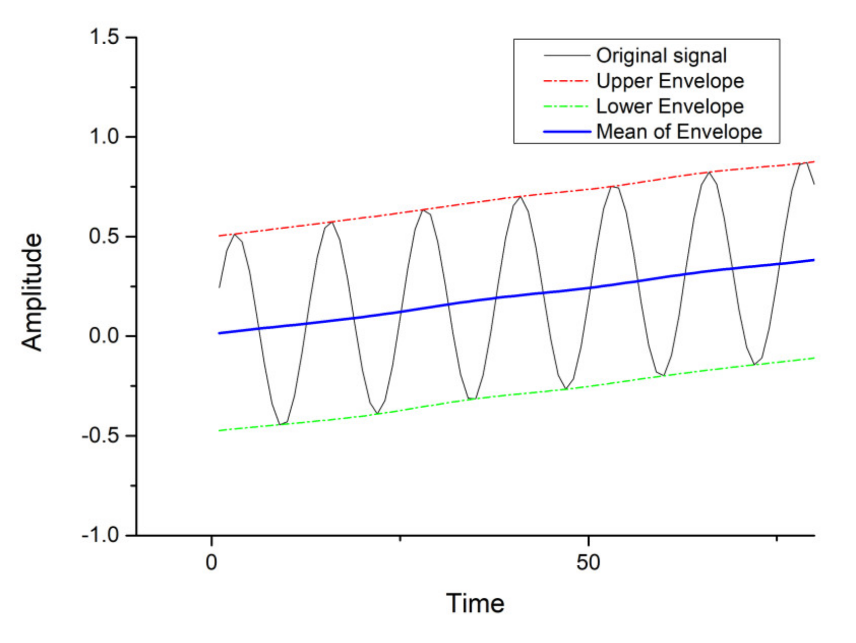
- Find out all the maxima and minima of the original signal A, and fit the upper, lower envelopes and a mean line M(t) of the original data with three spline interpolation functions. The distribution of the three lines is shown in Figure 1.
- 2.
- Subtract the original data A from the mean M(t) of the envelopes. If the new data meets the IMF constraints, the data is the IMF.
- 3.
- The result of subtracting the original data from the IMF is the residue data. Using the residue data as the new data and repeating the above process, the next IMF can be obtained.where is the residue after K-th decomposition.
- Add the Gaussian white noise to the original data.
- The decomposition of EMD is performed to obtain the IMF components.
- Repeat steps 1 and 2, adding a new normal distribution white noise data each time.
- Integrating the obtained IMFs according to the order to get the mean, each component of EEMD can be obtained.
- Generate a particular white noise and add it to original signal: Here represent the original signal and is the first white noise of finite variance. Then, we extract all the IMFs from the new series by EMD. The mean of these IMFs is the first mode of CEEMDAN.here, n represent the number of modes, while (j=1,2,……n) indicates the whole modes decomposed by EMD. is the first mode of CEEMDAN and equal to the mean of .
- 2.
- Calculate the first-order residue:
- 3.
- Decompose the residue to get the second-order IMF and calculate the second-order residue:
- 4.
- Decompose the k-th residue and extract the first mode, and the k-th mode can be obtained using the following equation (k = 2, 3, …K):
2.2. RNN, LSTM, MRNN and MLSTM
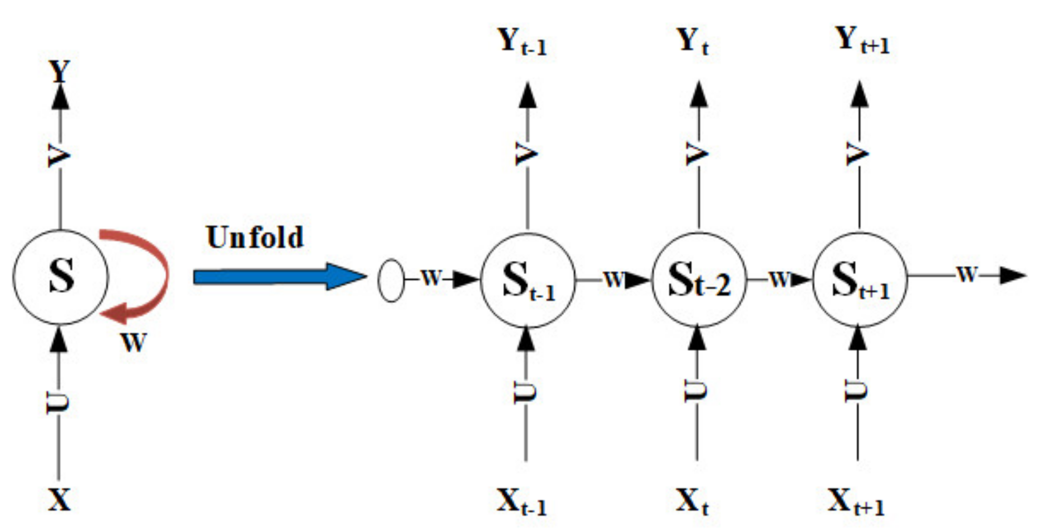
2.2.1. RNN
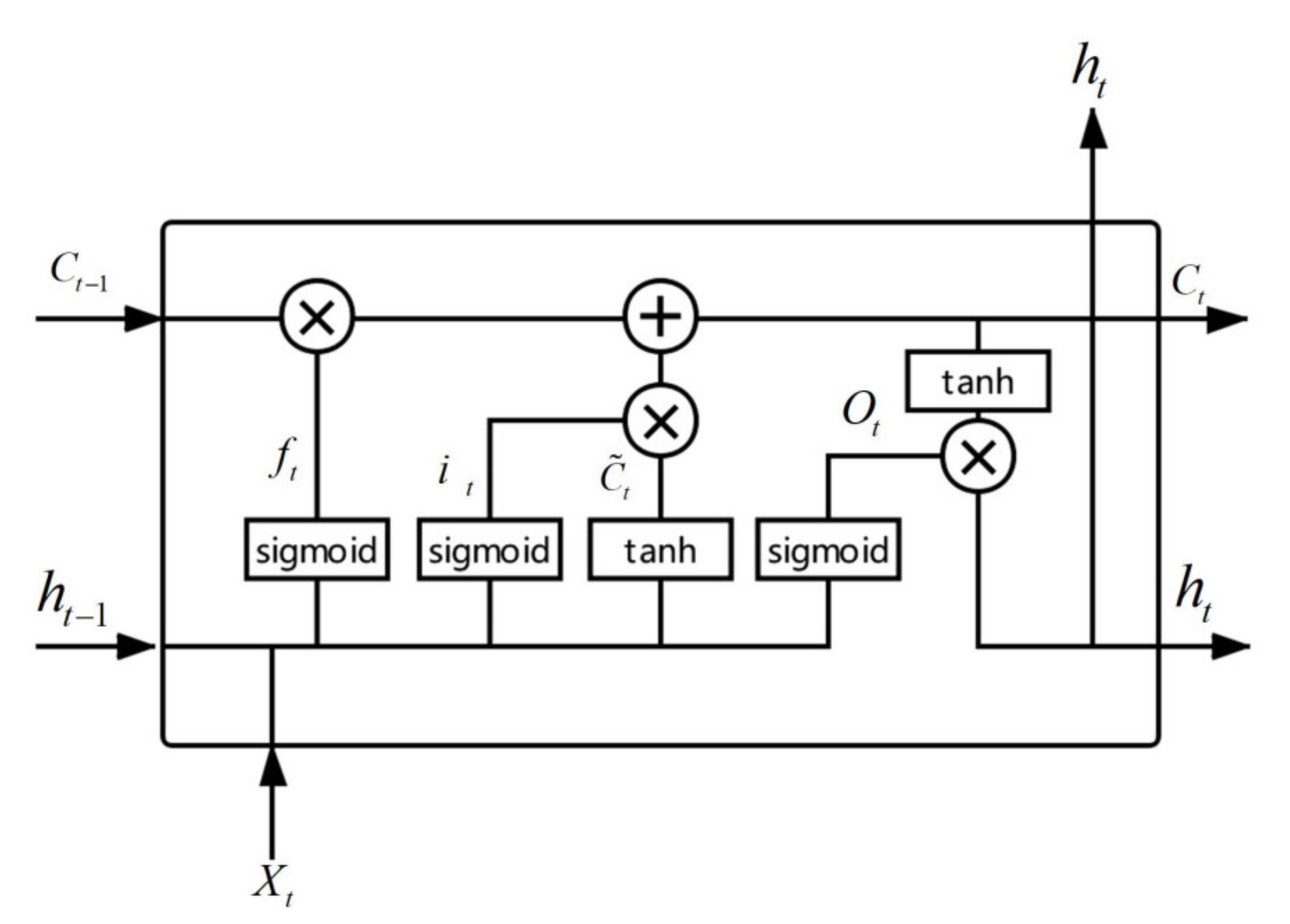
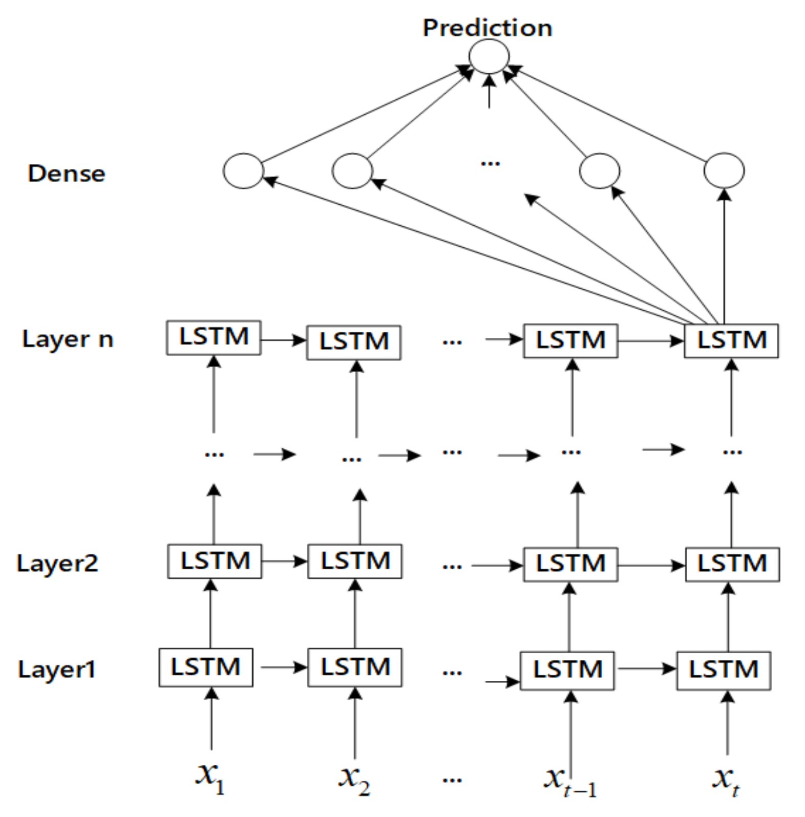
2.2.2. LSTM
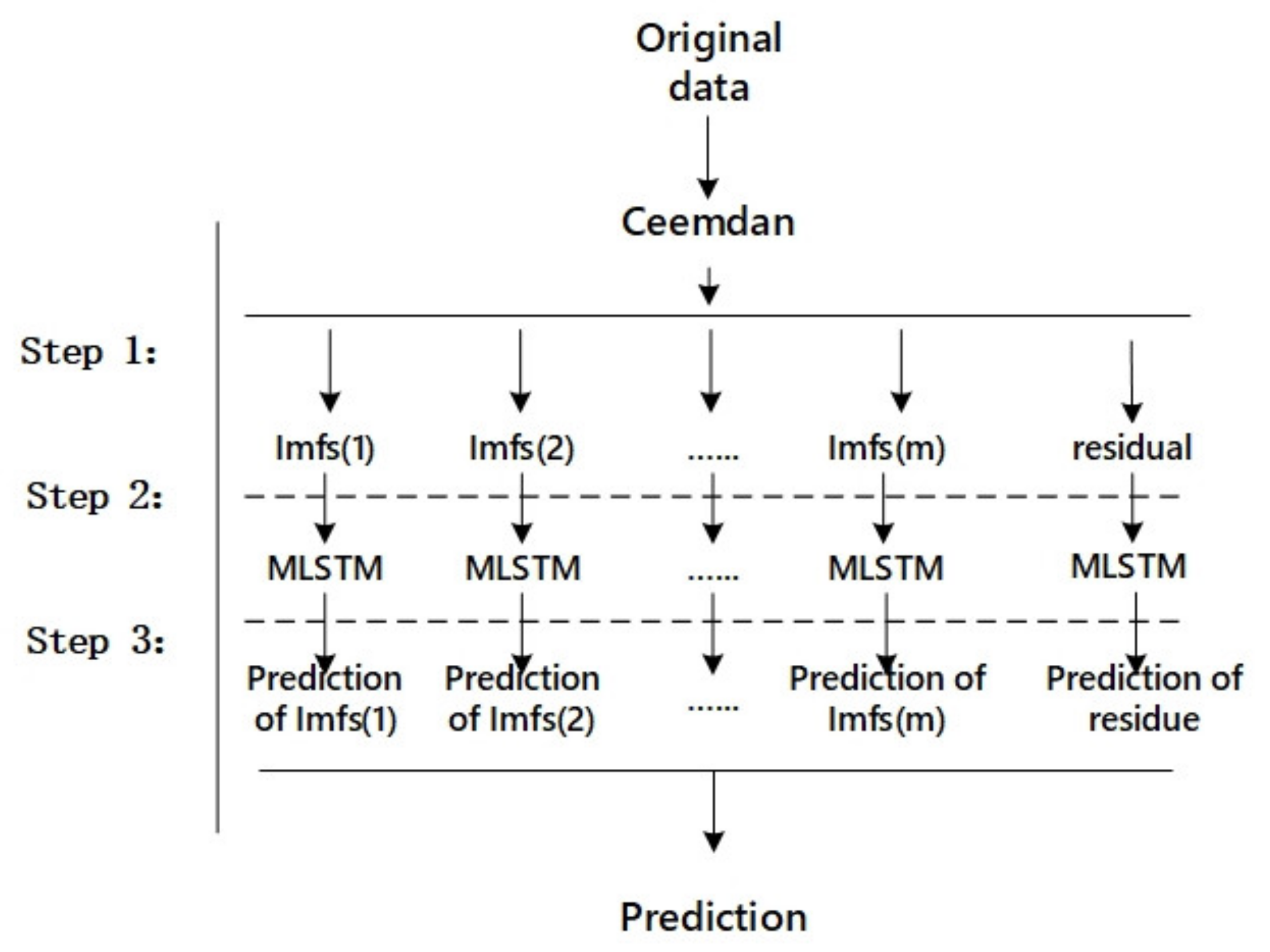
2.2.3. CEEMDAN–MLSTM
- Decompose the original data into relatively simple IMFs by CEEMDAN.
- Input the IMFs into the multilayer LSTM neural network separately and predict each extracted IMF.
- Finally, sum up the IMF and residual of each training. Then, we get the expected prediction.
3. Experiment
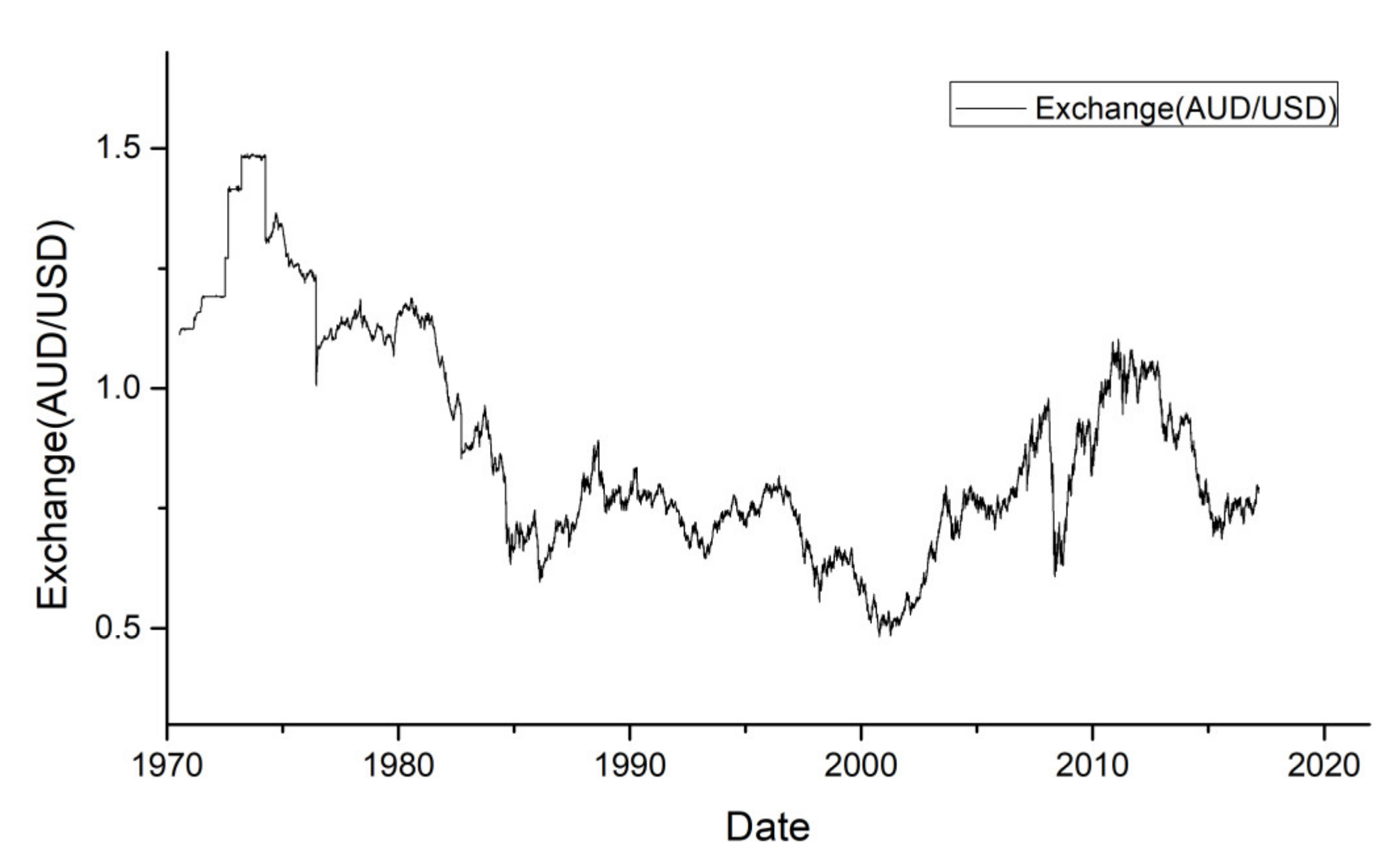
3.1. Data Preparing and Description
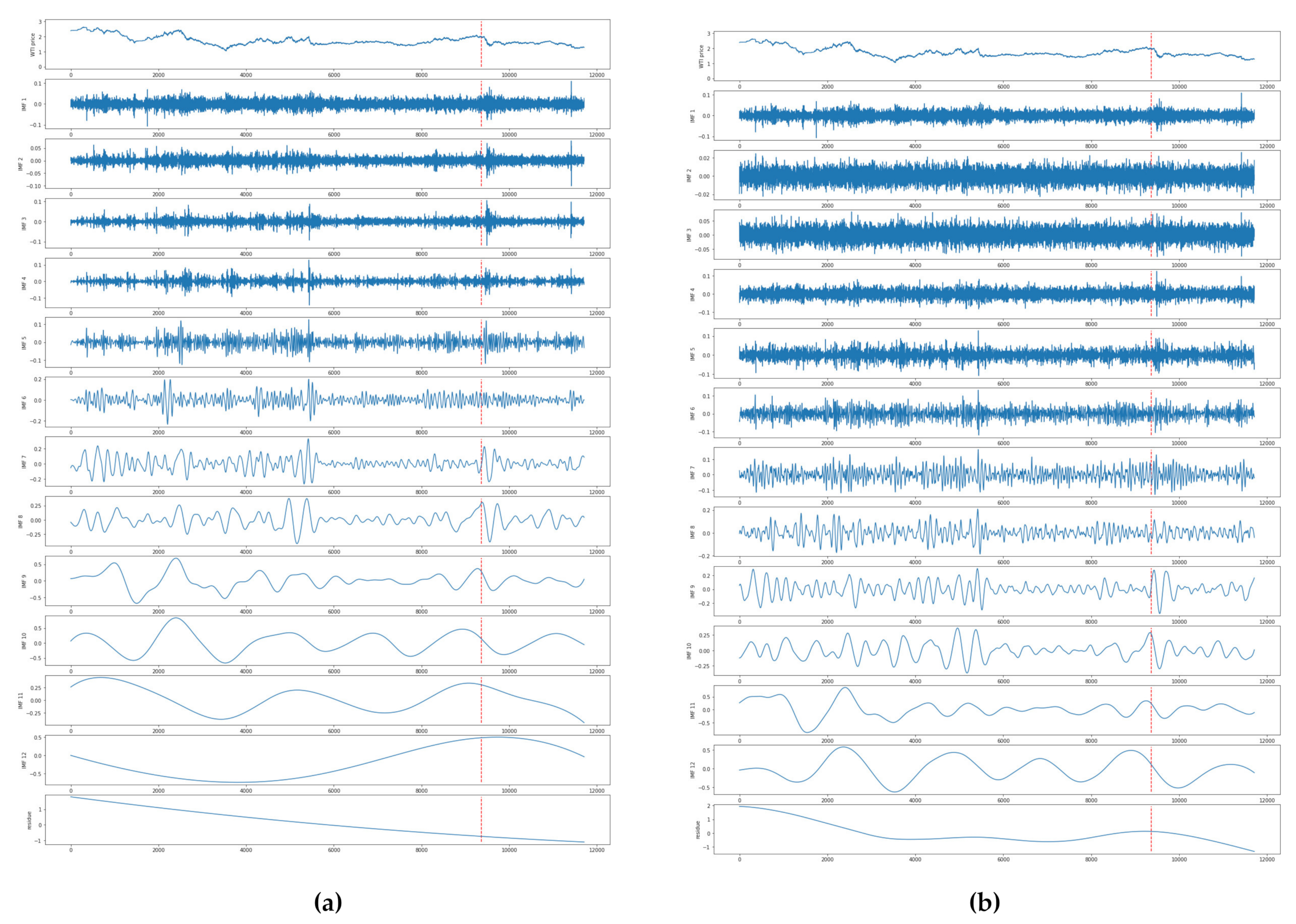
3.2. Data Decomposition
3.3. Building of MLSTM
3.3.1. Loss
3.3.2. Learning Rate
3.3.3. Batch_size
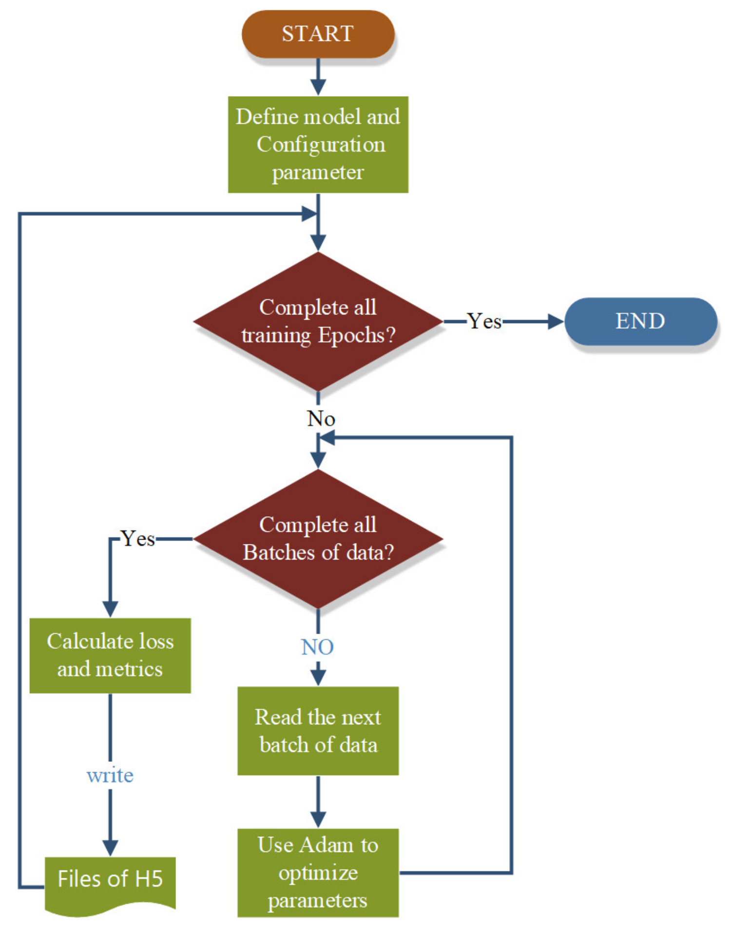
3.3.4. Optimizer
3.3.5. Metrics
- MAE:
- 2.
- RMSE:
- 3.
- MAPE:
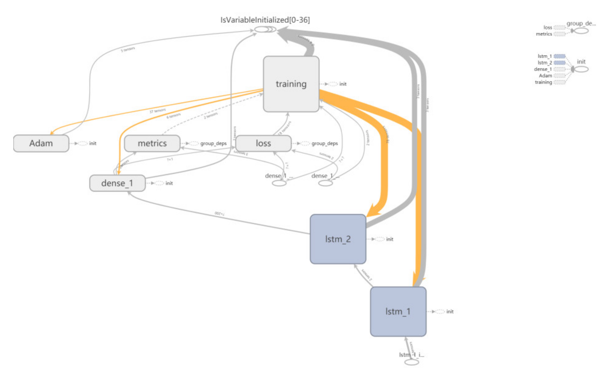
3.3.6. Dependencies in MLSTM
3.4. Experimental Results and Analysis
3.4.1. Prediction and Analysis Based on Undecomposed Data
3.4.2. Prediction and Analysis Based on Decomposition Data
- Decompose the three preprocessed identical exchange rate data by EMD, EEMD, and CEEMDAN methods to obtain three sets of different IMFs.
- Divide each group of IMFs into training set and test set, and input the training set into RNN, MRNN, LSTM, and MLSTM models for training.
- Enter the test data set and observation values into the trained deep learning model to obtain the final evaluation result.
3.5. Discussion
3.5.1. Performance of Different Step-Ahead Forecasts
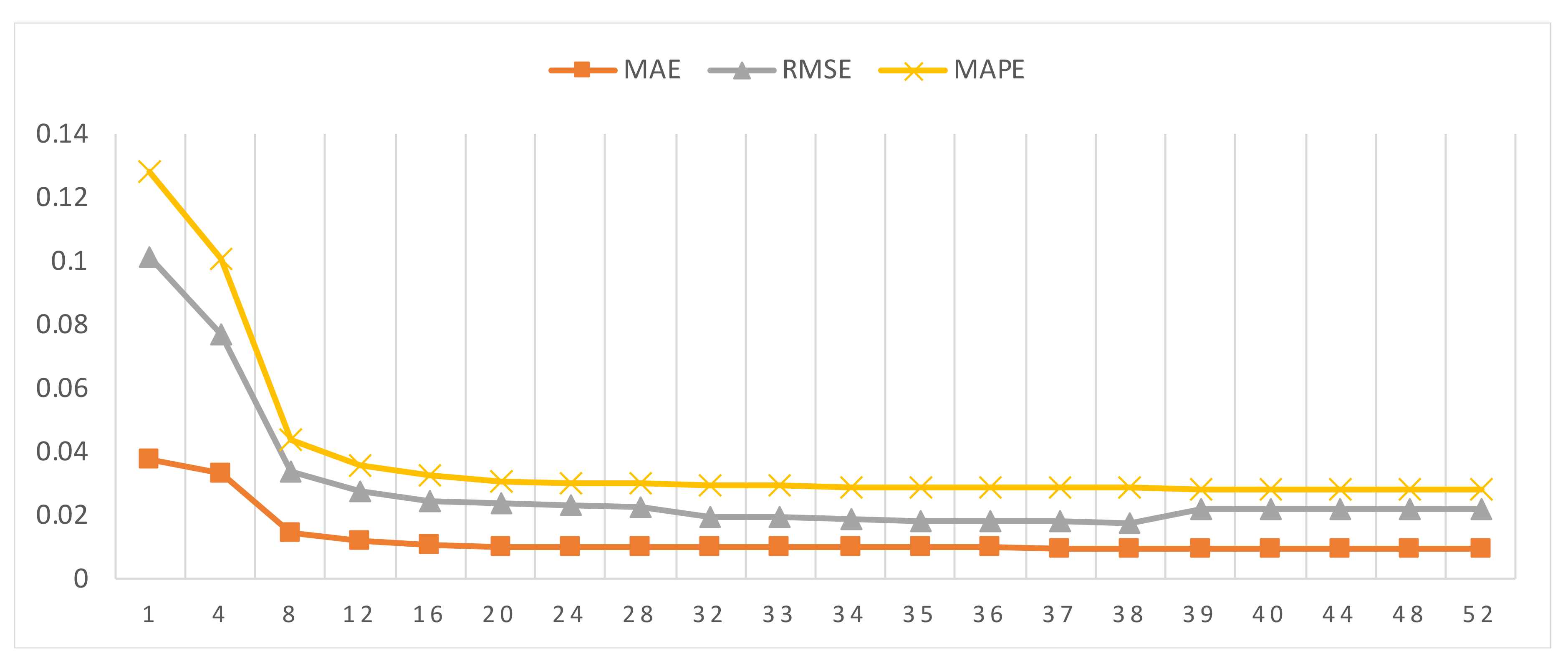
3.5.2. Impact of Different Lag Orders
4. Conclusions
Author Contributions
Funding
Conflicts of Interest
References
- Brada, J.C.; Méndez, J.A. Exchange rate risk, exchange rate regime and the volume of international trade. Kyklos 2007, 41, 263–280. [Google Scholar] [CrossRef] [Scilit]
- Korhonen, A. Strategic financial management in a multinational financial conglomerate: A multiple goal stochastic programming approach. Eur. J. Oper. Res. 2001, 128, 418–434. [Google Scholar] [CrossRef] [Scilit]
- Takatoshi, I.; Satoshi, K.; Kiyotaka, S.; Junko, S. Exchange rate exposure and exchange rate risk management: The case of japanese exporting firms. Discuss. Pap. 2013, 41, 17–29. [Google Scholar]
- Papaioannou, M.G. Exchange rate risk measurement and management: Issues and approaches for firms. IMF Work. Pap. 2006, 6, 1–20. [Google Scholar] [CrossRef] [Scilit]
- Davidson, J.; Li, X. Strict stationarity, persistence and volatility forecasting in ARCH(∞) processes. J. Empir. Financ. 2016, 38, 534–547. [Google Scholar] [CrossRef] [Scilit]
- Kristjanpoller, W.; Minutolo, M.C. Forecasting volatility of oil price using an artificial neural network-GARCH model. Expert Syst. Appl. 2016, 65, 233–241. [Google Scholar] [CrossRef] [Scilit]
- Riesgo García, M.V.; Krzemień, A.; Manzanedo del Campo, M.Á.; Escanciano García-Miranda, C.; Sánchez Lasheras, F. Rare earth elements price forecasting by means of transgenic time series developed with ARIMA models. Resour. Policy 2018, 59, 95–102. [Google Scholar] [CrossRef] [Scilit]
- Fan, J.; Yao, Q. Nonlinear Time Series: Nonparametric and Parametric Methods. J. Am. Stat. Assoc. 2005, 100, 348–349. [Google Scholar]
- Box, G. Box and jenkins: Time series analysis, forecasting and control. In A Very British Affair: Six Britons and the Development of Time Series Analysis during the 20th Century; Mills, T.C., Ed.; Palgrave Macmillan UK: London, UK, 2013; pp. 161–215. [Google Scholar]
- Engle, R.F. Autoregressive conditional heteroscedasticity with estimates of the variance of United Kingdom inflation. Econometrica 1982, 50, 987–1007. [Google Scholar] [CrossRef] [Scilit]
- Bollerslev, T. Generalized autoregressive conditional heteroskedasticity. EERI Res. Pap. 1986, 31, 307–327. [Google Scholar] [CrossRef] [Scilit]
- Lin, L.; Fang, W.; Xie, X. Random forests-based extreme learning machine ensemble for multi-regime time series prediction. Expert Syst. Appl. An Int. J. 2017, 83, 164–176. [Google Scholar] [CrossRef] [Scilit]
- Cao, L. Support vector machines experts for time series forecasting. Neurocomputing 2003, 51, 321–339. [Google Scholar] [CrossRef] [Scilit]
- Yan, D.; Qi, Z.; Wang, J.; Na, Z. Bayesian regularisation neural network based on artificial intelligence optimisation. Int. J. Prod. Res. 2016, 55, 2266–2287. [Google Scholar] [CrossRef] [Scilit]
- Rather, A.M.; Agarwal, A.; Sastry, V.N. Recurrent neural network and a hybrid model for prediction of stock returns. Expert Syst. Appl. 2015, 42, 3234–3241. [Google Scholar] [CrossRef] [Scilit]
- Hsieh, T.-J.; Hsiao, H.-F.; Yeh, W.-C. Forecasting stock markets using wavelet transforms and recurrent neural networks: An integrated system based on artificial bee colony algorithm. Appl. Soft Comput. 2011, 11, 2510–2525. [Google Scholar] [CrossRef] [Scilit]
- Rosas-Romero, R.; Díaz-Torres, A.; Etcheverry, G. Forecasting of stock return prices with sparse representation of financial time series over redundant dictionaries. Expert Syst. Appl. 2016, 57, 37–48. [Google Scholar] [CrossRef] [Scilit]
- Zhou, T.; Gao, S.; Wang, J.; Chu, C.; Todo, Y.; Tang, Z. Financial time series prediction using a dendritic neuron model. Knowl. Based Syst. 2016, 105, 214–224. [Google Scholar] [CrossRef] [Scilit]
- Mammadli, S. Financial time series prediction using artificial neural network based on Levenberg-Marquardt algorithm. Procedia Comput. Sci. 2017, 120, 602–607. [Google Scholar] [CrossRef] [Scilit]
- Kim, H.Y.; Won, C.H. Forecasting the volatility of stock price index: A hybrid model integrating LSTM with multiple GARCH-type models. Expert Syst. Appl. 2018, 103, 25–37. [Google Scholar] [CrossRef] [Scilit]
- Guresen, E.; Kayakutlu, G.; Daim, T.U. Using artificial neural network models in stock market index prediction. Expert Syst. Appl. 2011, 38, 10389–10397. [Google Scholar] [CrossRef] [Scilit]
- Bisoi, R.; Dash, P.K. A hybrid evolutionary dynamic neural network for stock market trend analysis and prediction using unscented Kalman filter. Appl. Soft Comput. 2014, 19, 41–56. [Google Scholar] [CrossRef] [Scilit]
- Ma, Z.; Dai, Q.; Liu, N. Several novel evaluation measures for rank-based ensemble pruning with applications to time series prediction. Expert Syst. Appl. 2015, 42, 280–292. [Google Scholar] [CrossRef] [Scilit]
- Gong, X.; Si, Y.-W.; Fong, S.; Biuk-Aghai, R.P. Financial time series pattern matching with extended UCR suite and support vector machine. Expert Syst. Appl. 2016, 55, 284–296. [Google Scholar] [CrossRef] [Scilit]
- Pwasong, A.; Sathasivam, S. A new hybrid quadratic regression and cascade forward backpropagation neural network. Neurocomputing 2016, 182, 197–209. [Google Scholar] [CrossRef] [Scilit]
- Wang, J.; Peng, B.; Zhang, X. Using a stacked residual LSTM model for sentiment intensity prediction. Neurocomputing 2018, 322, 93–101. [Google Scholar] [CrossRef] [Scilit]
- EA-LSTM: Evolutionary attention-based LSTM for time series prediction. Knowl. Based Syst. 2019, 181, 104785. [CrossRef] [Scilit]
- Liu, G.; Guo, J. Bidirectional LSTM with attention mechanism and convolutional layer for text classification. Neurocomputing 2019. [Google Scholar] [CrossRef] [Scilit]
- Sagheer, A.; Kotb, M. Time series forecasting of petroleum production using deep LSTM recurrent networks. Neurocomputing 2019, 323, 203–213. [Google Scholar] [CrossRef] [Scilit]
- Dai, S.; Li, L.; Li, Z. Modeling vehicle interactions via modified LSTM models for trajectory prediction. IEEE Access 2019, 7, 38287–38296. [Google Scholar] [CrossRef] [Scilit]
- Hao, X.; Du, Q.H.; Mark, R. SS-LSTM: A Hierarchical LSTM Model for Pedestrian Trajectory Prediction. In Proceedings of the IEEE Winter Conference on Applications of Computer Vision. IEEE, 2018, Lake Tahoe, NV, USA, 12–15 March 2018. [Google Scholar]
- Tang, L.; Dai, W.; Yu, L.; Wang, S. A Novel CEEMD-Based EELM Ensemble Learning Paradigm for Crude Oil Price Forecasting. Int. J. Inf. Technol. Decis. Mak. 2015, 14, 141–169. [Google Scholar] [CrossRef] [Scilit]
- Cao, J.; Li, Z.; Li, J. Financial time series forecasting model based on CEEMDAN and LSTM. Phys. A Stat. Mech. Its Appl. 2018. [Google Scholar] [CrossRef] [Scilit]
- Huang, N.E.; Shen, Z.; Long, S.R.; Wu, M.L.C.; Shih, H.H.; Zheng, Q.N.; Yen, N.C.; Tung, C.C.; Liu, H.H. The empirical mode decomposition and the Hilbert spectrum for nonlinear and nonstationary time series analysis. Proc. R. Soc. A Math. Phys. Eng. Sci. 1998, 454, 903–995. [Google Scholar] [CrossRef] [Scilit]
- Wu, Z.; Huang, N. Ensemble empirical mode decomposition: A noise-assisted data analysis method. Adv. Adapt. Data Anal. 2009, 1, 1–41. [Google Scholar] [CrossRef] [Scilit]
- Zhang, N.; Lin, A.; Shang, P. Multidimensional k-nearest neighbor model based on EEMD for financial time series forecasting. Phys. A Stat. Mech. Its Appl. 2017, 477, 161–173. [Google Scholar] [CrossRef] [Scilit]
- Das, A.B.; Bhuiyan, M.I.H. Discrimination of focal and non-focal EEG signals using entropy-based features in EEMD and CEEMDAN domains. In Proceedings of the 9th International Conference on Electrical and Computer Engineering (ICECE), Dhaka, Bangladesh, 20–22 December 2016. [Google Scholar]
- Pradeepkumar, D.; Ravi, V. Forecasting financial time series volatility using Particle Swarm optimization trained quantile regression neural network. Appl. Soft Comput. 2017, 58, 35–52. [Google Scholar] [CrossRef] [Scilit]
- Meese, R.A.; Rogoff, K. Empirical exchange rate models of the seventies: Do they fit out of sample? J. Int. Econ. 1983, 14, 3–24. [Google Scholar] [CrossRef] [Scilit]
- Galeshchuk, S. Neural networks performance in exchange rate prediction. Neurocomputing 2016, 172, 446–452. [Google Scholar] [CrossRef] [Scilit]
- Wright, J.H. Bayesian model averaging and exchange rate forecasts. J. Econom. 2008, 146, 329–341. [Google Scholar] [CrossRef] [Scilit]
- Jia, S.; Guo, Y.; Qiang, W.; Jian, Z. Trend extraction and similarity matching of financial time series based on emd method. In Proceedings of the World Congress on Computer Science & Information Engineering, Los Angeles, CA, USA, 31 March–2 April 2009. [Google Scholar]



| Parameter | Description |
|---|---|
| spline_kind | Defines type of spline, which connects extrema |
| nbsym | Number of extrema used in boundary mirroring |
| max_imf | IMF number to which decomposition should be performed |
| ensemble_size | Number of trials or EMD performance with added noise |
| noise_strength | Standard deviation of the Gaussian random numbers used as additional noise. |
| Method | nbsym | max_imf | trials | noise_width/epsilon |
|---|---|---|---|---|
| EMD | 2 | ALL | -- | -- |
| EEMD | 2 | ALL | 100 | 0.05 |
| CEEMDAN | 2 | ALL | 100 | 0.05 |
| Model | Number of Hidden Layers | Number of Hidden Units | MAE | RMSE | MAPE(%) |
|---|---|---|---|---|---|
| ARIMA | - | - | 0.087 | 0.116 | 6.148 |
| Bayesian | - | - | 0.034 | 0.038 | 2.327 |
| SVM | - | - | 0.035 | 0.040 | 2.629 |
| RNN | 1 | 200 | 0.032 | 0.036 | 2.598 |
| MRNN | 2 | 200,200 | 0.023 | 0.025 | 1.836 |
| LSTM | 1 | 200 | 0.020 | 0.021 | 1.614 |
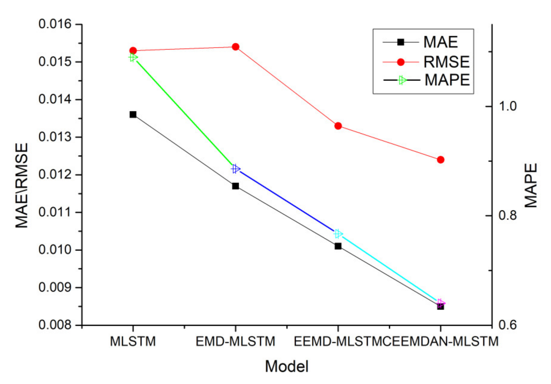
| MLSTM | 2 | 200,200 | 0.014 | 0.015 | 1.090 |
| Model | Number of Hidden Layers | No. of Hidden Units | MAE | RMSE | MAPE |
|---|---|---|---|---|---|
| EMD-RNN | 1 | 200 | 0.017 | 0.023 | 0.01304 |
| EMD-MRNN | 2 | 200,200 | 0.021 | 0.025 | 0.01590 |
| EMD-LSTM | 1 | 200 | 0.020 | 0.024 | 0.01456 |
| EMD-MLSTM | 2 | 200,200 | 0.012 | 0.015 | 0.00886 |
| Model | Number of Hidden Layers | Number of Hidden Units | MAE | RMSE | MAPE |
|---|---|---|---|---|---|
| EEMD-RNN | 1 | 200 | 0.022 | 0.018 | 0.0136 |
| EEMD-MRNN | 2 | 200,200 | 0.013 | 0.016 | 0.0095 |
| EEMD-LSTM | 1 | 200 | 0.013 | 0.017 | 0.0101 |
| EEMD-MLSTM | 2 | 200,200 | 0.010 | 0.013 | 0.0077 |
| Model | Number of Hidden Layers | Number of Hidden Units | MAE | RMSE | MAPE |
|---|---|---|---|---|---|
| CEEMDAN-–RNN | 1 | 200 | 0.111 | 0.015 | 0.0083 |
| CEEMDAN–MRNN | 2 | 200,200 | 0.012 | 0.016 | 0.0088 |
| CEEMDAN–LSTM | 1 | 200 | 0.014 | 0.011 | 0.0091 |
| CEEMDAN–MLSTM | 2 | 200,200 | 0.009 | 0.012 | 0.0064 |
| MAE Horizon | Methods | |||
|---|---|---|---|---|
| CEEMDAN–MLSTM | CEEMDAN–LSTM | CEEMDAN–MRNN | CEEMDAN–RNN | |
| One | 0.0096 | 0.0145 | 0.0124 | 0.1116 |
| Two | 0.0124 | 0.0153 | 0.0161 | 0.0252 |
| Three | 0.0203 | 0.0232 | 0.0306 | 0.0317 |
| Four | 0.0406 | 0.0543 | 0.0589 | 0.0411 |
| RMSE Horizon | CEEMDAN–MLSTM | CEEMDAN–LSTM | CEEMDAN–MRNN | CEEMDAN–RNN |
| One | 0.0122 | 0.0157 | 0.0168 | 0.0157 |
| Two | 0.0143 | 0.0183 | 0.0206 | 0.0241 |
| Three | 0.0189 | 0.0259 | 0.0317 | 0.0345 |
| Four | 0.0559 | 0.0625 | 0.0646 | 0.0759 |
| MAPE Horizon | CEEMDAN–MLSTM | CEEMDAN–LSTM | CEEMDAN–MRNN | CEEMDAN–RNN |
| One | 0.0064 | 0.0091 | 0.0088 | 0.0083 |
| Two | 0.0109 | 0.0118 | 0.0133 | 0.0147 |
| Three | 0.0347 | 0.0412 | 0.0462 | 0.0512 |
| Four | 0.1056 | 0.1263 | 0.1502 | 0.1753 |
© 2020 by the authors. Licensee MDPI, Basel, Switzerland. This article is an open access article distributed under the terms and conditions of the Creative Commons Attribution (CC BY) license (http://creativecommons.org/licenses/by/4.0/).
Share and Cite
Lin, H.; Sun, Q.; Chen, S.-Q. Reducing Exchange Rate Risks in International Trade: A Hybrid Forecasting Approach of CEEMDAN and Multilayer LSTM. Sustainability 2020, 12, 2451. https://doi.org/10.3390/su12062451
Lin H, Sun Q, Chen S-Q. Reducing Exchange Rate Risks in International Trade: A Hybrid Forecasting Approach of CEEMDAN and Multilayer LSTM. Sustainability. 2020; 12(6):2451. https://doi.org/10.3390/su12062451
Chicago/Turabian StyleLin, Hualing, Qiubi Sun, and Sheng-Qun Chen. 2020. "Reducing Exchange Rate Risks in International Trade: A Hybrid Forecasting Approach of CEEMDAN and Multilayer LSTM" Sustainability 12, no. 6: 2451. https://doi.org/10.3390/su12062451
APA StyleLin, H., Sun, Q., & Chen, S.-Q. (2020). Reducing Exchange Rate Risks in International Trade: A Hybrid Forecasting Approach of CEEMDAN and Multilayer LSTM. Sustainability, 12(6), 2451. https://doi.org/10.3390/su12062451