Coal Resource Security Assessment in China: A Study Using Entropy-Weight-Based TOPSIS and BP Neural Network

Abstract

Energy security has become a worldwide issue in recent years. Coal resources security (CRS), an important part of energy security, has been an emerging concern in many countries, due to the diminishing fossil energy reserve and unbalanced energy structure. However, there is no universally agreed method of constructing indicator system for CRS assessment. Subjectivity in the process of evaluation also affects the results of assessment. Moreover, CRS is a complex system that should be evaluated scientifically under diverse methods. Therefore, we constructed an indicator system and evaluation model of CRS and used a case study of China and 31 provinces in its mainland to evaluate CRS at both national and provincial levels. The indicator system included two subsystems—long-term CRS and short-term CRS. We also chose a few elements and factors that are consistent with China’s reality. Different research methods were used: the entropy-weight-based TOPSIS (Technique for Order Preference by Similarity to an Ideal Solution) method is applied to evaluate the degree of CRS, which avoids the subjectivity of weight determination and reflects the relative merit of each indicator; the BP (Back-Propagation) Neural Network method is used to analyze the sensitivity of CRS to each index. The results show that the national level of CRS dropped in the early years but slowly picked up with the help of government intervention. Investment in coal industry development resulted in the immediate effect of improving CRS. The positive impact of maintaining environmental sustainability is stable over either the short, medium, or long term. The degrees of CRS vary significantly across provinces, even between those with similar coal stock levels. Extra attention should be paid to the transportation of coal resources among provinces and intervention to balance supply and demand within the regions.

1. Introduction

Energy security is crucial to the sustainable development of all countries and always rises high on the policy agenda of governments, considering its linkages with economic growth, trade openness, and the ecological environment [1]. However, due to diminishing fossil energy reserves, the increasing pressure of environmental protection, and a changing energy structure [2], the outlook for global energy security is not optimistic. To ensure energy security, a global race to develop renewable energy has begun [3]. Different countries are developing policies that facilitate technological innovation and open new horizons for global energy [4,5].

As a developing country with rapid economic growth, China faces a unique energy dilemma [6]. Its energy structure is extremely unbalanced: two-thirds of its energy consumption is provided by coal. The high reliance on coal makes the coal strategy a primary concern of policy makers [7]. Further, the objective assessment and understanding of coal resource status are the basis for making relevant government policy. Therefore, in this article, we will carry out an evaluation of coal resources security (CRS) in China.

China’s CRS situation is complicated. Fossil energy usage (mainly coal) results in China suffering enormous pressure from environmental pollution and climate problems [8]. There are many conflicts and contradictions in the development and utilization of coal resources, including the overcapacity of coal resources, the unreasonable allocation of coal resources in time and space [9], etc. As coal imports increase, China is closely connected to the international market, which means it is vulnerable to international terrorism and global geopolitical risks [10]. In such a complex context, many scholars have come to understand the CRS from different perspectives and have obtained different results. Hou et al. [11] calculated CRS from four aspects—resource security, development conditions, the ecological environment, and the coal market. They used CRS to give warning about coal consume quantity and production ability. Guo et al. [12] established a Pressure-State-Response (PRS) model to evaluate and predict CRS, and their results showed that, after 2009, CRS did not repeat its previous rising cycle and reached a maladjustment state from 2009 to 2016. This article shares the same turning point with our work. Gao and Li [13] established a measurement system through four interlocking steps—coal production, circulation, international trade, and consumption. Wang et al. [14] analyzed coal availability, accessibility, sustainability, and technology development and synthesized CRS with these four variables. Chao et al. [15] based CRS on coal supply and usage, paying more attention to the problems brought by coal usage. Jing Xua et al. [16] took CRS as symbol of sustainable development and found that economic growth in China was largely dependent on coal consumption.

The above literature shows that the research on CRS varies with the authors’ understanding. Actually, there is no universally agreed method of constructing indicator system for CRS assessment. The definition of CRS is slippery, and it can hold multiple dimensions and present different specificities depending on the district, timeframe, or energy type. This uncertainty makes it difficult to identify consistent research methods for analysis, prediction, and policy making [17]. In this paper, our understanding of CRS is an extension of the definition of energy security from the International Energy Agency (IEA), which is widely accepted and appears in many articles [18,19,20,21]. We define CRS as the uninterrupted availability of coal resources at an affordable price. We can also use long-term CRS and short-term CRS to summarize the influence factors.

Based on this definition of CRS, we will build CRS evaluation system to calculate the CRS degree. Considering the regional differences and multiple layers of coal policies in China, we will study CRS at both the overall level and the provincial level [22]. Finally, a back-propagation (BP) neural network model for prediction [23,24] will be built to simulate the non-linear relationships in the evaluation system and calculate indicators’ sensitivity to CRS. We want to achieve the following objectives through the above empirical test. First, we want to observe annual trends in CRS. Second, by sensitivity analysis, we want to find key variables that affect CRS. Third, we want to clearly delineate low-CRS areas and high-CRS areas. This work, we believe, will help policy makers to design a coal industry strategy and arrange overall coal production.

This study makes the following contributions. First, after extending the definition of energy security given by the IEA, we summarize a comprehensive set of factors affecting CRS. Second, we differentiate the indicator system of evaluation between national and provincial levels. Last but not least, it combines a back-propagation neural network with factor sensitivity analysis. The structure of this paper is as follows. Section 2 introduces the indicator system and evaluation methods. Section 3 shows the result of CRS at both the national and provincial levels. Section 4 presents the conclusions.

2. Research Method

2.1. Indicator System for CRS at the Provincial and National Levels

Coal resource security (CRS) is a multifaceted concept. Inspired by the definition of energy security from the International Energy Agency (IEA), we define CRS as the uninterrupted availability of coal resources at an affordable price, which involves long-term CRS and short-term CRS.

Long-term CRS is affected by three elements—coal reserves, the development level of the coal industry, and environment sustainability. They reflect whether the supply and use of coal resources will be limited in the long run. Coal reserves affect the self-sufficiency of coal resources. The development level of the coal industry indicates the capacity of coal production, thus affecting the supply and use of coal resources in the medium and long term. The destruction to the environment caused by coal production and consumption increases the economic cost of using coal in the long run. We should not ignore the fact that that environmental pressure is the driving factor to reduce the use of fossil fuels and develop clean energy [5].

Short-term CRS is affected by three elements—coal supply, coal demand, and coal import and export. Coal supply refers to domestic coal capacity, which determines to what extent China can achieve coal self-sufficiency. Coal demand refers to the minimum requirement for the coal supply. Increases in coal demand may indicate that a country is more dependent on coal and has fewer alternative energy sources. The factor of coal import and export reflects the ability to acquire external coal resources and control the balance of supply and demand by reacting promptly to emergencies such as a shortage of external coal supply or overly volatile prices in the international market. Coal imports have a negative impact on national coal resource security, in that a large quantity of coal imports is detrimental to the domestic coal industry, leading to high dependence on overseas coal resources and low self-sufficiency.

Based on the analysis of the definition of coal resource security, this paper sets four tiers in the index system. The first tier is the ultimate goal of our research—CRS. The second tier includes the two subsystems. The third tier includes the primary indicators affecting the subsystems, as discussed above. The fourth tier includes secondary indicators linked closely with the front indicators, some of which are flow and stock data and some are elasticity indexes reflecting sensitivity.

In order to evaluate the degree of CRS at national and provincial levels, we establish two indicator systems for evaluation [25].

The indicators at the national level are shown in

Table 1. The indicator system of national coal resource security (CRS).

Target	Subsystem	Primary Indicator	Secondary Indicators	Impact Direction
National CRS	Long-term CRS	Coal Reserves	N1: Proved coal reserves	+
			N2: Base coal reserves	+
		Development level of Coal Industry	N3: Output of special mining equipment	+
			N4: Investment in coal mining industry	+
			N5: Energy industry investment	+
			N6: The ratio of coal mining industry investment in the total energy industry investment	+
		Environment sustainability	N7: SO2 emission	−
			N8: Investment in waste gas treatment projects	+
	Short-term CRS	Coal supply	N9: Elasticity coefficient of coal production	+
			N10: Coal production	+
		Coal demand	N11: Coal consumption	−
			N12: The ratio of Thermal power generation to the total power generation	−
			N13: The ratio of coal consumption to domestic energy	−
		Coal import and export	N14: Coal self-sufficiency ratio	+
			N15: Net coal import	−

. Among them, the elasticity coefficient of coal production N9 refers to the average annual growth rate of total coal production divided by the average annual growth rate of the national economy. Coal self-sufficiency ratio N14 refers to coal production divided by coal consumption. Data for the other indicators are directly available from our database. Table 1 also lists the impact direction of each factor on national CRS. Among them, all indexes for coal reserves (N1 and N2), development level of coal industry (N3, N4, N5, and N6), and coal supply (N9 and N10) are hypothesized to have positive effects on CRS, while all the indicators for coal demand (N11, N12, and N13) have a negative impact. In terms of environment sustainability, SO₂ emission (N7) has a negative impact on CRS because high pollution leads to higher social and economic cost. However, the investment of waste gas treatment projects (N8) improves environment sustainability and thus has a positive impact on CRS. The coal self-sufficiency ratio (N14) indicates the ability of the country to satisfy its coal demand and thus is consistent with CRS, while net coal import (N15) is detrimental to the self-sufficiency ratio, and thus, a negative direction should be identified.

We do not consider carbon dioxide emissions as a secondary indicator because the technology of carbon dioxide (CO₂) capture and storage (CCS) is still immature, and policies such as carbon credits, carbon taxes, and other incentives to increase the cost of coal use are still in operation on a small scale, so it is difficult to measure the actual increase in the cost of coal usage caused by CO₂ emissions [26,27]. However, SO₂ emissions from coal can be avoided by coal washing, which increases the cost of coal use in practice.

Table 2. The indicator system of provincial CRS.

Target	Subsystem	Primary Indicator	Secondary Indicators	Impact Direction
Provincial CRS	Long-term CRS	Coal Reserves	M1: Base coal reserves	+
		Development level of Coal Industry	M2: The ratio of coal mining industry investment to the total energy industry investment	+
			M3: The ratio of the fixed assets investment of state-owned coal mining industry to the total investment of state-owned economic energy	+
		Environment sustainability	M4: SO2 emission	−
	Short-term CRS	Coal demand	M5: The total amount of coal transfer	−
			M6: The ratio of Thermal power generation to the total power generation	−
			M7: Coal consumption	−
		Coal supply	M8: Coal production	+
			M9: The total amount of coal available for deployment	+
			M10: The outward allocation of coal	+
		Coal import and export	M11: Net coal import	−

shows the evaluation system of coal resource security at provincial level. Compared with Table 1, we add some indicators to reflect the movement of coal resources between provinces (M5, M9 and M10).

The total amount of inward deployment of coal (M5) refers to the amount of coal received from the other provinces, which indicates a negative situation of CRS. The total amount of coal available for deployment (M9) refers to the total output of key state-owned coal mines in each province. The amount of outward deployment of coal (M10) refers to the ratio of the total amount that can be allocated to other provinces. These two indicators are consistent with the capacity of coal resources within the province, so they have a positive impact on the CRS.

2.2. Evaluation Methods

2.2.1. The Entropy-Weight-Based TOPSIS

The methods for evaluation of indicator system vary extensively, including the method based on Catastrophe theory [28], the analytic hierarchy process [29], the principal component analysis [18], and the entropy-weight-based TOPSIS (Technique for Order Preference by Similarity to an Ideal Solution) [29,30,31,32,33,34]. The entropy-weight-based TOPSIS method has been widely applied in the field of evaluation and management since the 1980s and has become a classic method in multi-index comprehensive evaluation. The entropy-weight method is advantageous because it avoids the arbitrariness of subjective determination of indicators’ weights and has strong adaptability in the process of weight determination [31,34,35,36,37]. TOPSIS was first proposed by Wang and Yoon in 1981 for evaluation and decision-making problems. It is a comparative method of analyzing the difference between each object and its optimal solution. It has no special requirement for sample data and can be combined with many other methods. Therefore, we apply this method in our article.

The specific steps of entropy-weight-based TOPSIS method are as follows:

• Formulate a matrix $M={[m_{ij}]}_{p\times q}$, with p evaluation objects and q evaluation indicators. In order to make different indicators comparable, we standardize each index and get the normalized matrix $Z={[z_{ij}]}_{p\times q}$.
• Use the entropy weight method to calculate weights of each index. First, calculate the proportion of the i^th target indicator value under the j^th indicator: $v_{ij}=\frac{z_{ij}}{{\displaystyle \sum _{i=1}^p{z}_{ij}}}$. Then, use $v_{ij}$ to calculate the information entropy of j^th indicator $e_j=-h{\displaystyle \sum _{i=1}^p{v}_{ij}}\ln v_{ij}$, where $h$ is a positive number and can be set as $h=1/\ln p$. Next, calculate the coefficient of difference of j^th indicator $g_i=1-e_i$. Finally, the weight for the j^th evaluation index can be expressed as $w_j=\frac{g_j}{{\displaystyle \sum _{j=1}^p{g}_j}}$.
• Determine the correlation between each indicator and the final evaluation target—coal resource security. If it is positive, the optimal solution is the maximum value of the indicator, and the worst solution is the minimum value of the indicator, and vice versa if it is negative. A positive ideal solution $E^{+}$ is formed by all the optimal values and a negative ideal solution $E^{-}$ is formed by all the worst values.
• Calculate the Euclidean distances from evaluation object to the positive ideal solutions or negative ideal solutions using the following equations:

  $$D_i^{+}=\sqrt{{\displaystyle \sum _{j=1}^p{w}_j{(z_j^{+}-z_j)}^2}},D_i^{-}=\sqrt{{\displaystyle \sum _{j=1}^p{w}_j{(z_j^{-}-z_j)}^2}}$$
• Calculate the relative approach degree for all the evaluation objectives using $C_i=\frac{D_i^{+}}{D_i^{+}+D_i^{-}}$, in which the larger the $C_i$, the lower the comprehensive evaluation, and vice versa. The level of coal resource security can be evaluated based on the value of 1-$C_i$. The larger the value of 1-$C_i$, the better the situation of coal resource security.

2.2.2. Back-Propagation (BP) Neural Network

Neural network is a calculation model that simulates the biological nervous system for decision making and prediction. In this article, the BP neural network is used to simulate the relationship between the secondary indicators (from the CRS evaluation system) and CRS degree, so that we can get the resulting predictive value under any given secondary indicators. Back-propagation neural network can find the non-linear correlation in data sets. Compared with other prediction models, such as the grey model [33,38], the BP neural network algorithm is able to adapt, generalize, and tolerate faults. It has been used in various prediction problems [31,32,39]. That is why it is an effective prediction model, and we can apply this model to find the reaction of CRS when changing one input indicator.

The functionality of the neural network is determined by its network structure and connection weights between neurons. The first step in predicting is to train a neural network model to minimize the loss function $f$. The loss function includes two parts—the error term and the regular term. The error term measures the degree of fitting of the neural network model on the training data set, while the regular term measures the complexity of the model to prevent over-fitting.

The value of the loss function is determined by the two parameters of the model: weight value $P={[p_{ij}]}_{n_1\times n_2}$ and offset value $B={[b_{ij}]}_{n_1\times 1}$, where $n_1$ is the number of neurons, and $n_2$ is the number of neurons in the previous layer (or the number of input layer features). We combine $P$ and $B$ into an n-dimensional weight vector $W=[w_1,w_2,\dots ,w_n],n=n_1(n_2+1)$. Therefore, the loss function can be expressed as $f(W)$. $W*$ is the minimum value of the loss function. By arbitrarily selecting a point $A$ in space, we can calculate the first-order and second-order derivatives of the loss function. The first order derivative can be expressed as a vector:

$$gradf{(W)}_i={f^{\prime }}_i(W)=\frac{df}{d{w}_i},(i=1,\dots ,n)$$

Similarly, the second order derivative can be expressed as a Hessian matrix:

$$H_{ij}(f(W))=\frac{d^{2}f}{d{w}_{i}d{w}_j},(i,j=1,\dots ,n)$$

Therefore, the training problem of the neural network is transformed into the problem of solving the multivariable continuous differentiable function. We abstract the learning problem of the neural network into the problem of finding the parameter vector $W*$, so that the loss function $f(W)$ reaches the minimum value at this point. Suppose that we find the minimum point of the loss function, then the gradient of the neural network function is considered to be equal to zero. Usually, the loss function is a non-linear function. Therefore, we search step by step in the parameter space to find the optimal solution. In each step, the parameters of the neural network model are recalculated, and the value of $f(W)$ are correspondingly reduced. The specific method is as follows: first, randomly initialize a set of model parameters; then, update the set of parameters iteratively so the loss function value decreases; and finally, when a specific condition or termination condition is met, the entire training process ends.

Common training algorithms include gradient descent, Newton’s method, conjugate gradient, the quasi-Newton method, and the Levenberg–Marquardt (LM) algorithm. In this paper, the Levenberg–Marquardt algorithm, also known as the least square method of attenuation, is applied to find the squared error in the loss function. It is efficient even when the size of data is small.

The iterative process of LM algorithm is as follows:

• Set the training error allowable value $\epsilon$, the initialization weight $W_n$ and the number of iterations $n$, as the weight correction parameter $[\lambda ,v]$. Generally, $\lambda$ is a small number. $v$ takes a number greater than 1. Set the initial $n=0$.
• Calculate the output value $t_n$ of the network, then calculate the error ${\epsilon }_n$.
• Calculate the Jacobian matrix $J$.
• Base on $[\lambda ,v]$ and $W_n$ to calculate the weight correction amount $\Delta W_n$, and get the weight correction value $W_{n+1}=W_n+\Delta W_n$.
• If the error ${\epsilon }_n$ satisfies the accuracy requirement, go to (7); otherwise, calculate the new error ${\epsilon }_{n+1}$ with the weight correction value $W_{n+1}$.
• If the new error ${\epsilon }_{n+1}$ is smaller than the old error, let $n=n+1$ and $\lambda =\lambda \times v$ and return to (2); otherwise, if the weight value is not updated this time, the new weight $W_{n+1}$ is equal to the old weight $W_n$, the weight correction parameter is changed to $\lambda =\lambda \times v$, and return to (4).
• Stop.

2.2.3. Sensitivity Analysis

The sensitivity analysis of input parameters studies the change of output parameters when given input parameters are changed in a certain baseline state—that is, the influence of the change of input parameters on the output parameters. The calculation process is as follows. First, normalize all input indicators to [0,1]. A single input variable is tested with the values 0, 0.25, 0.5, 0.75, and 1, while the other input variables remain unchanged. After introducing each test value of the input index into the network, observe the value of the output index given by the neural network, record the maximum and minimum outputs, and calculate the ratio of their difference to the maximum output. The mean of all the ratios is the sensitivity of the input variable. In this process, the values of the other variables are the calculating benchmarks. The sensitivity values are different against different benchmarks. This difference reflects the joint effect of all the input variables.

3. Results

3.1. National CRS Assessment

Our study period is from 2004 to 2017. During these 14 years, the overall situation of coal in China has significantly changed. Base coal reserves have fallen by 80 billion tons in 14 years. If the rate of coal use continues at the same level, China’s coal reserves will be exhausted in 30 years. In the past decade, with the development of the economy, the investment in the coal industry has increased year by year, leading to the problem of coal overcapacity. In addition, for the first time in recent years, China’s coal industry has seen a sharp decline in investment in mining because of the country’s policy to reduce excess capacity. The ratio of coal mining industry investment in the total energy industry investment has also declined year by year since 2011. SO₂ emission decreased by 50% in the last five years. The share of thermal power generation has declined significantly in the past five years. Coal consumption and production continue to rise with the development of the economy. China’s coal self-sufficiency rate has been decreasing since 2008, while net coal imports have been increasing for many years.

For a more comprehensive assessment of coal resources, in this part, we used the entropy-weight-based TOPSIS to evaluate and analysis the degree of coal resource security in China at national level during 2004–2017. Then, we trained the back-propagation neural networks and combine it with sensitivity analysis, so we can understand the influence mechanism in our national CRS system further.

3.1.1. Calculation of National CRS

Our data were extracted from National Bureau of Statistics, China Coal Information Network, and China Customs, covering the time period 2004–2017.

First, the entropy weight method was used to calculate the weight of each index. According to the normalized matrix, positive ideal scheme A+ and negative ideal scheme A− in the finite scheme (14 years) are obtained.

Table 3. Weight, positive solution, and negative solution of indicators in national CRS system.

Index	Weight	Positive Ideal Solution	Negative Ideal Solution	Index	Weight	Positive Ideal Solution	Negative Ideal Solution
N1	0.0300	0.9862	−2.6474	N9	0.0324	1.5203	−2.5005
N2	0.0721	0.9502	−1.5892	N10	0.0547	1.1747	−1.8295
N3	0.1019	1.1970	−1.3033	N11	0.0404	2.2088	0.9646
N4	0.0670	1.2121	−1.6103	N12	0.0643	−1.7319	1.2183
N5	0.0670	1.4259	−1.5917	N13	0.0491	−1.9845	1.0164
N6	0.0783	1.6964	−1.4366	N14	0.0911	1.5594	−1.3440
N7	0.0383	−2.3682	1.0711	N15	0.0960	−1.3251	1.4272
N8	0.1172	2.1759	−1.0682

shows that the average weights of indexes under two factors—development level of coal industry (N3, N4, N5, and N6) and coal import and export (N14 and N15) are the largest. N3 (the proportion of investment in state-owned coal mining industry in total energy investment) and N8 (investment in waste gas projects) have the largest two weights, which indicates that these two indicators have more information and play a more important role in the evaluation of national CRS.

The Euclidean distances D+ and D− were calculated respectively. Then, the relative proximity of each evaluation object to the positive ideal scheme C was calculated. Here, 1-C represents the comprehensive evaluation of national CRS degree. The results are plotted in Figure 1, from which we identify the changing direction of CRS degree in China during the data period. The national CRS increased with slightly fluctuation from 2004 to 2009 and reached its peak in 2007. From 2009 to 2015, it gradually declined, but recovered after 2015.

Here is our analysis combined with economic facts and relevant policies (we assume that the policy lag is only one to two years):

(1)

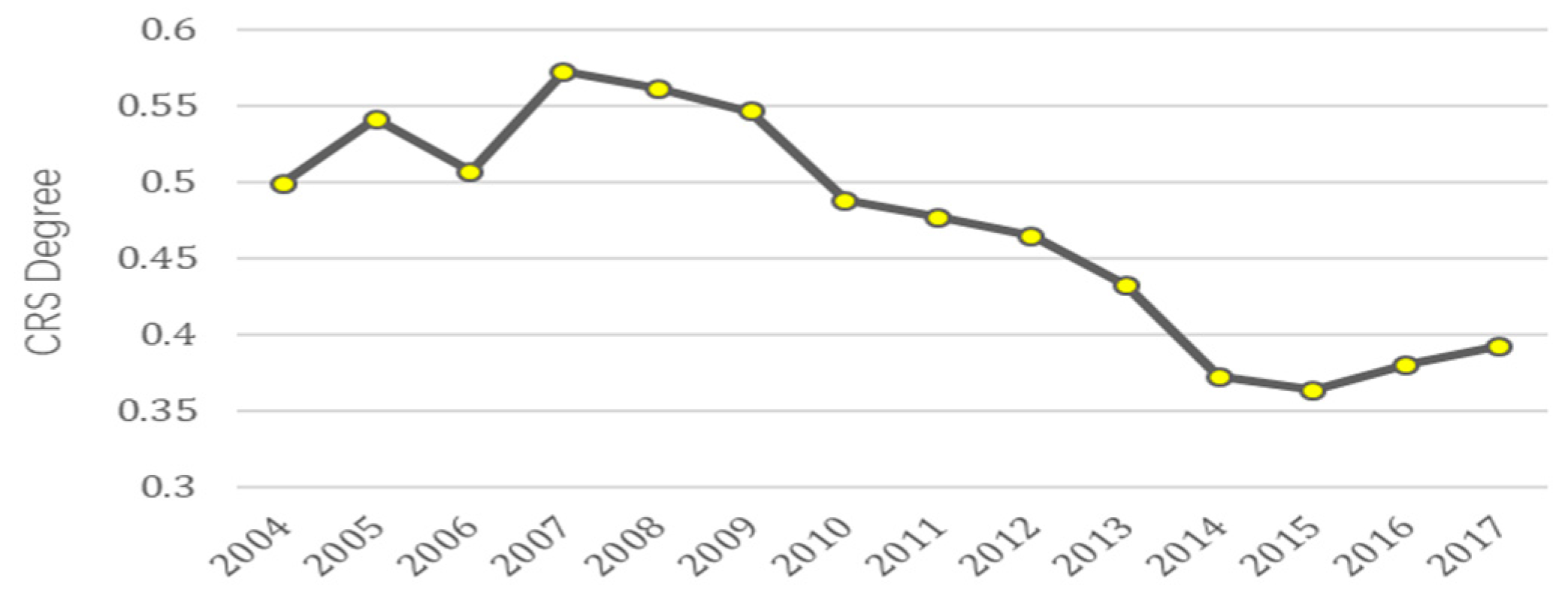
From 2004 to 2008, influenced by the upward economic trend and the country’s vigorous construction of infrastructure, the demand for coal increased greatly, which led to the development of the coal industry. By calculating the Euclidean distance D+ from the primary indicators to their positive ideal solutions (see

Table 4. The Euclidean distance D+ from the primary indicator to its positive ideal solution.

Year	Coal Reserves	Development Level of Coal Industry	Environment Sustainability	Coal Demand	Coal Supply	Coal Import and Export
2017	0.6706	0.9753	0.3474	0.3410	0.0846	1.1516
2016	0.3454	0.8033	0.1612	0.3459	0.5695	0.7921
2015	0.3742	0.4250	0.3607	0.4057	0.2245	1.2863
2014	0.4209	0.2012	0.1866	0.5495	0.1859	1.4952
2013	0.5270	0.0643	0.2760	0.7332	0.1005	1.2235
2012	0.1757	0.0684	1.0727	0.7386	0.1027	0.6330
2011	0.1002	0.2097	1.2632	1.0418	0.0234	0.6224
2010	0.0243	0.3911	1.3315	0.6956	0.0793	0.3966
2009	0.0060	0.7504	1.1921	0.8775	0.1600	0.0948
2008	0.0012	1.1453	1.1321	0.6753	0.2458	0.1002
2007	0.0015	1.4400	1.1718	1.1198	0.2626	0.0601
2006	0.0001	1.7246	1.3661	1.0257	0.3268	0.0304
2005	0.0004	1.9962	1.4134	0.9110	0.3782	0.0076
2004	0.0010	2.3750	1.5277	0.7092	0.4938	0.0040

), we found that from 2004 to 2008, the development level of the coal industry had moved the most towards the positive ideal solution. So, it contributed most to the change of national CRS. The fluctuation of coal demand’s D+ caused the fluctuation of CRS. We believe that the period from 2004 to 2008 was the golden development period of the coal industry, and the coal supply was gradually improved, so the CRS during this period climbed step by step.

(2)

From 2008 to 2012, under the government’s Four Trillion Plan, the rapid growth of the coal industry and coal supply led to a glut of coal stocks that China’s domestic market could not absorb. Though the Table 4, we found that the D+ of coal demand didn’t change much; the huge increase in the D+ of coal import and export had exacerbated the contradiction between domestic coal supply and demand. The imbalance put some pressure on the national CRS. We think that the period from 2008 to 2012 was the adjustment period for coal industry, and CRS slightly decreased.

(3)

From 2012 to 2014, the coal industry was oversaturated, and the economic downturn led to a reduction in coal demand, which intensified the contradiction between coal supply and demand. In these three years, the incremental D+ of coal import and export contributed most to the negative change of national CRS. We think that the period from 2012 to 2014 was the winter for coal industry, and CRS sharply declined. And we should also notice the positive contribution of environmental sustainability to CRS.

(4)

From 2015 to 2017, national policies and the operating pressure of coal industry had led to the closure of overcapacity and backward coal producers. Some policies also drove a decline in coal import and coal industry investment, which reduced the gap between supply and demand for coal. Margins in the coal economy also started to recover. In Table 4, we can see the D+ of all four primary indicators to its fluctuated during the three years, and their mutual cooperation helped the national CRS to recover slowly. We think that the period from 2015 to 2017 was the recovery period for coal industry, and CRS slightly picked up.

3.1.2. Sensitivity Analysis

In 2019, the National Development and Reform Commission formulated overall coal planning and systematic arrangements to be implemented by 2025. They aimed to construct an efficient system of coal production, supply, and marketing and provide solutions to the potential problems within the system, which would ensure China’s coal industry to gradually move toward a controllable and predictable future. So, an empirical prediction of the situation of coal resource security in China is able to provide help for policy makers in determining energy strategies.

The back-propagation neural network model was applied to predict the security of coal resources in China. We normalized 14-year data of the 15 indicators as the input data. Fourteen-year CRS degrees obtained from the Entropy-weight-based TOPSIS method were used as the prediction variables (output variables). The 14 samples from 14 years were divided into a training set (85%) and a test set (15%) randomly in the process of training, which are shown in the

Table A1. Normalized input variables.

	Index	2017	2016	2015	2014	2013	2012	2011	2010	2009	2008	2007	2006	2005	2004
Input data	N1	0.3633	0.2751	0.2322	0.1991	0.1687	0.1160	0.0000	0.5232	0.8488	0.9079	0.9078	0.9682	0.9613	1.0000
	N2	0.2322	0.1991	0.1687	0.1160	0.0000	0.5232	0.8488	0.9079	0.9078	0.9682	0.9613	1.0000	0.9742	0.9541
	N3	1.0000	0.9726	0.8727	0.9592	0.9475	0.8084	0.5591	0.5117	0.3001	0.1350	0.1274	0.0533	0.0000	0.0506
	N4	0.4184	0.5016	0.7086	0.8535	0.9663	1.0000	0.9011	0.6612	0.5057	0.3651	0.2381	0.1642	0.1010	0.0000
	N5	0.9772	1.0000	0.9891	0.9478	0.8489	0.7104	0.6135	0.5575	0.4726	0.3490	0.2445	0.1706	0.1066	0.0000
	N6	0.0000	0.0796	0.3130	0.5086	0.7459	0.9821	1.0000	0.7100	0.5720	0.4944	0.3794	0.3155	0.2435	0.0757
	N7	0.0000	0.1328	0.5741	0.6414	0.6820	0.7252	0.7835	0.7643	0.7813	0.8437	0.9295	1.0000	0.9770	0.8051
	N8	0.4693	0.6475	0.5862	1.0000	0.7704	0.1777	0.1065	0.0702	0.1387	0.1901	0.2049	0.1399	0.1085	0.0000
	N9	0.6747	0.0000	0.3562	0.4066	0.5620	0.5574	0.8196	0.7368	0.6797	0.6079	0.6903	0.7144	0.9009	1.0000
	N10	0.7569	0.6958	0.8774	0.9460	1.0000	0.9843	0.8865	0.7050	0.5359	0.4214	0.3441	0.2415	0.1307	0.0000
	N11	0.9155	0.9105	0.9401	0.9860	1.0000	0.9536	0.9221	0.7366	0.6620	0.5663	0.5374	0.3833	0.2310	0.0000
	N12	0.0000	0.0323	0.1538	0.3592	0.5643	0.5516	0.8513	0.6559	0.7561	0.5550	1.0000	0.9737	0.9006	0.8652
	N13	0.0000	0.1344	0.2727	0.4298	0.5785	0.6694	0.8099	0.7273	0.9256	0.9174	1.0000	0.9917	0.9917	0.8099
	N14	0.1050	0.2467	0.0612	0.0000	0.0908	0.3235	0.3262	0.4402	0.7031	0.6961	0.7576	0.8228	0.9074	1.0000
	N15	0.8589	0.6999	0.9154	1.0000	0.8997	0.6221	0.6135	0.4631	0.1934	0.2007	0.1435	0.0930	0.0370	0.0000
Target data	CRS degree	0.3922	0.3798	0.3634	0.3721	0.4319	0.4646	0.4763	0.4877	0.5461	0.5609	0.5720	0.5066	0.5407	0.4988c

.

We used Neural Network Toolbox in MATLAB (a software from MathWorks Company in Natick, Massachusetts, USA) to train our BP neural network model. First, we need to set the structure of the Neural Network. The number of nodes in the input layer is 15, corresponding to the 15 indexes in the coal resource security evaluation index system. Set the number of network hidden layers to 1. According to the calculation formula of the number of neuronal nodes in the hidden layer, $n_1=\sqrt{n_2+l}+\alpha$ (where $n_2$ is the number of nodes in the input layer, $l$ is the number of hidden layers, $\alpha \in [1,10]$ ), the number of nodes should be between 5 and 11. After testing the number of different hidden layer nodes, it was finally determined that the number of selected nodes in this paper is 10. The number of nodes in the output layer is 1, and the output object is the degree of CRS. The next step is to determine the parameters of the neural network. The LM algorithm is applied to train the neural network. The target is that the MSE of the training set is less than 0.000001, and that of the test set is less than 0.0001. In our tests, the MSE of the training set turned out to be 1.28241 × 10⁻⁷, and that of the test set was 4.67832 × 10⁻⁵, which met our accuracy requirements.

Next, we calculated and sorted the sensitivities of output parameters to changes in input parameters under the neural network model. We selected three calculating benchmarks which are 2017, 2013–2017, and 2004–2017, to calculate single-term average, medium-term average, and long-term average sensitivities, respectively. Take N1’s sensitivity as an example. We use five numbers (0, 0.25, 0.7, 0.75, 1) to replace the valuation of N1 in 2017 to get five different samples for the input of BP Neural Network model. After inputting them to the trained model, we can get five outputs for the prediction of CRS degree. Then, we record the maximum and minimum outputs and take the ratio of their difference to the maximum output as sensitivity of N1 in 2017 and also as the single-term sensitivities of N1. N1’s medium-term average sensitivity is the average of N1’s sensitivities from 2013 to 2017. N1’s long-term average sensitivity is the average of N1’s sensitivities from 2004 to 2017. The results are shown in the Figure 2.

By comparing the sensitivities for different lengths of term, we find the following:

(1)

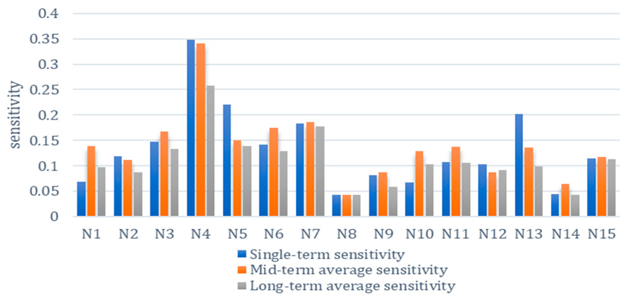
The single-term sensitivities of indexes for coal industry development (N4 and N5) are higher than their medium-term and long-term average sensitivities, which indicates that the positive impact of development in the coal industry takes effect immediately within the first year, while being compromised by the changes in the other indexes in later years.

(2)

The sensitivities of indexes for environment sustainability (N7 and N8) in the single, medium, and long terms are stable, which indicates that they work independently. Therefore, we can draw the conclusion that regardless of changes in any other indexes, investment in environment sustainability always has a positive impact on CRS.

(3)

The mid-term average sensitivities of most indexes, even those related to short-term CRS (N9, N10, N14, and N15), are higher than their single-term and long-term average sensitivities, which indicates that they are more influential in the period 2013–2017 than in the other years. This is not surprising considering the intensive government intervention starting from 2015.

3.2. Provincial CRS Assessment

The issues of uneven distribution of coal resources, mismatch of coal supply and coal demand between provinces, and difficulties in cross-regional allocation of coal have all threatened the security of coal resources. Therefore, we calculated the weights of indicators in our provincial evaluation system (in mainland China) from 2012 to 2016 and ranked the degrees of CRS of each province for each year. The data is from the National Bureau of Statistics, the China Energy Yearbook, and the China Coal Industry Yearbook. The weights are shown in Figure 3 and they vary over five years. In particular, note that the M5’s weight in 2014 is significantly different from other years.

Based on the weights we calculated the degrees of CRS in each province and sorted them for each year. We gave the ranks for the provinces according to their CRS degree. The results are presented in

Table 5. Rankings of the provincial CRS degree from 2012 to 2016.

Province	2012	2013	2014	2015	2016
Beijing	18	15	22	13	13
Tianjin	23	21	27	20	19
Hebei	25	26	15	26	26
Shanxi	1	1	1	1	1
Inner Mongolia	2	2	2	2	2
Liaoning	27	30	25	30	29
Jilin	20	25	24	24	22
Heilongjiang	17	22	13	21	17
Shanghai	24	23	26	22	24
Jiangsu	31	31	30	31	31
Zhejiang	29	27	28	27	28
Anhui	5	7	6	5	5
Fujian	22	18	21	15	21
Jiangxi	19	17	19	23	20
Shandong	28	28	17	29	30
Henan	16	19	7	12	25
Hubei	26	24	31	25	23
Hunan	14	11	11	10	10
Guangdong	30	29	29	28	27
Guangxi Zhuang Autonomous Region	21	20	23	19	18
Hainan	12	12	20	11	12
Chongqing	11	13	16	14	15
Sichuan	15	16	14	16	16
Guizhou	6	5	5	4	4
Yunnan	9	6	9	9	14
Tibet Autonomous Region	10	10	18	6	6
Shaanxi	3	3	3	3	3
Gansu	13	14	10	8	9
Qinghai	8	8	12	7	8
Ningxia Hui Autonomous Region	4	4	4	17	11
Xinjiang Uygur Autonomous Region	7	9	8	18	7

.

Our findings are as follows:

(1)

Shanxi, Inner Mongolia, Anhui, Guizhou, Yunnan, Shaanxi, and Xinjiang have remained in the top 10 provinces for all studied years because they are major coal producing provinces, with coal reserves and supplies far ahead of the rest of the provinces. Among them, Guizhou, as the only province in southern China that transfers coal resources and sends electricity from the west to the east, has been vigorously carrying out mergers, reorganizations, transformations, and upgrades of its coal mines since 2012. This explains its improved rankings in the last two years.

(2)

Tianjin, Liaoning, Jilin, Shanghai, Jiangsu, Zhejiang, Shandong, Hubei, and Guangdong all remained in the bottom 10. This is mainly because these provinces have large demand for coal, but their own coal supply cannot meet the need. Therefore, the transfer of coal from other provinces or other counties is relatively large.

(3)

The rankings of Henan, Shandong, Heilongjiang, and Ningxia decreased in 2015, mainly because the effective supply was insufficient, and the amount of coal transferred to other provinces dropped significantly. It reflects the contradiction between supply and demand in these provinces.

For more intuitive result, we made Figure 4. We can draw the following conclusions:

(1)

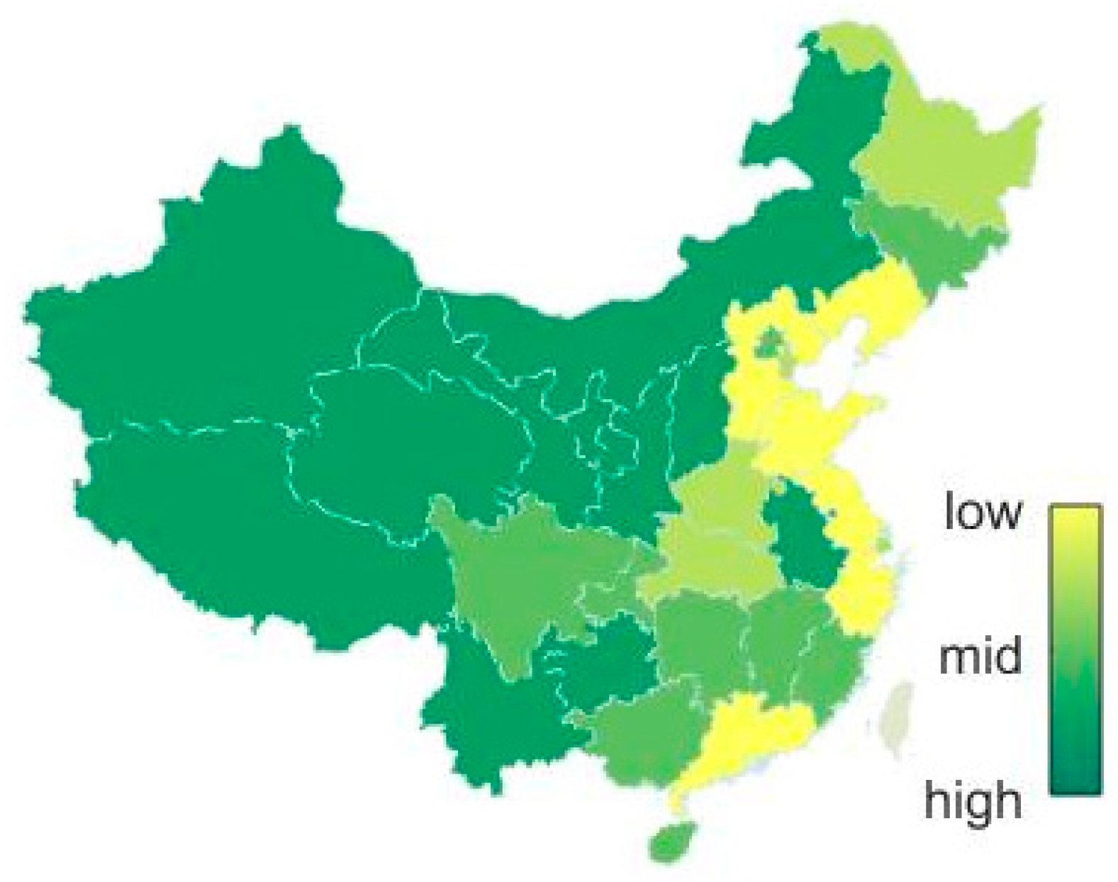
There are obvious regional differences in provincial CRS degree. CRS is quite low in the southeastern coastal provinces and high in the western and northern provinces. This characteristic also reflects that coal is mainly distributed in the inland areas and that the southeast coastal areas have large population, resulting in high coal demand.

(2)

Shanxi, Inner Mongolia, Shaanxi, Gansu, Ningxia Hui, and Xinjiang Uygur have high coal stocks. Among these provinces, Shanxi has the largest coal supply. This is because Shanxi has made a high investment in the coal industry for many years, and traffic to and from Shanxi is relatively convenient compared with other inland provinces. Therefore, other inland provinces who want to improve their coal supply capacity require supporting transportation facilities and necessary investment, which will reduce part of the cost for domestic coal, thus enhancing competitiveness and gradually expanding the internal market.

(3)

We find that the CRS of Fujian, Shandong, Hunan, and Guangdong have stayed at a same low level, which is mainly because these eastern and southeastern coastal provinces have a high dependence on other provinces. Therefore, the import restrictions for these provinces should be lowered during peak seasons of coal use.

4. Conclusions

In this paper, we set up an indicator system of CRS and evaluated the degree of CRS in China based on the entropy-weight-based TOPSIS method from 2004–2017. During the 14 years of the study period, CRS went through a golden period, an adjustment period, a decline period, and a recovery period. We also found that government intervention played an important role in improving CRS in China in recent years. Then, we tried to find indexes of high sensitivities to CRS based on the BP neural network model. After comparing the single-term (2017), medium-term (2013–2017), and long-term (2004–2017) results, we discovered that investment in coal industry development can take immediate effect within one year to improve CRS. This effect will be compromised in later years by changes in the other indexes. However, the positive impact of investment in environment sustainability is stable. In a word, the government can indirectly control CRS by adjusting the amount of investment in the coal industry. Environmental protection has a positive and stable effect on the safety of coal resources. Therefore, we should constantly increase investment in environmental protection and promote environmental protection policies.

Additionally, we adjust the indicator system of CRS to accommodate provincial data issues. We evaluated and ranked the degrees of provincial CRS with data from 2012 to 2016. It is surprising to find significant differences in CRS between provinces with similar coal reserve levels. For provinces with rich coal reserves, extra attention should be paid to setting up an efficient intervention system within the region and more investment in their transportation network. For those with low coal reserves but high coal demand, government restrictions on coal import should be lowered, especially during peak seasons of coal use.

Our article has some limitations. First, our data set is too small, and therefore, the time segments for analysis are too short. It will take a longer time to verify the results. Second, the CRS degrees we calculated are a function of the distance to the ideal target, and its size has practical significance only in a limited context. Third, this paper is too conservative in the selection of indicators, which may affect the effectiveness of the results. In the future, we need to improve or change the model to solve this problem.

References

- Shahbaz, M.; Hye, Q.M.A.; Tiwari, A.K.; Leitão, N.C. Economic growth, energy consumption, financial development, international trade and CO2 emissions in Indonesia. Renew. Sustain. Energy Rev. 2013, 25, 109–121. [Google Scholar] [CrossRef]
- Augutis, J.; Krikštolaitis, R.; Martišauskas, L.; Pečiulytė, S.; Žutautaitė, I. Integrated Energy Security Assessment. Energy 2017, 138, 890–901. [Google Scholar] [CrossRef]
- Zeppini, P.; Van Den Bergh, J.C.J.M. Global competition dynamics of fossil fuels and renewable energy under climate policies and peak oil: A behavioural model. Energy Policy 2020, 136, 110907. [Google Scholar] [CrossRef]
- Schmidt, T.S.; Sewerin, S. Technology as a driver of climate and energy politics. Nat. Energy 2017, 2, 1–3. [Google Scholar] [CrossRef]
- Watcharejyothin, M.; Shrestha, R.M. Regional energy resource development and energy security under CO2 emission constraint in the greater Mekong sub-region countries (GMS). Energy Policy 2009, 37, 4428–4441. [Google Scholar] [CrossRef]
- Tang, E.; Peng, C.Y. A macro- and microeconomic analysis of coal production in China. Resour. Policy 2017, 51, 234–242. [Google Scholar] [CrossRef]
- Guo, L.; Wu, C.; Yu, J. A study on simulating energy security system of China. Sci. Res. Manag. 2015, 36, 112–120. [Google Scholar]
- Lin, B.Q.; Sun, C.W. How can china achieve its carbon emission reduction target while sustaining economic growth? Soc. Sci. China 2011, 1, 64–76. [Google Scholar]
- Wang, C.; Ducruet, C. Transport corridors and regional balance in China: The case of coal trade and logistics. J. Transp. Geogr. 2014, 40, 3–16. [Google Scholar] [CrossRef]
- Odgaard, O.; Delman, J. China’s energy security and its challenges towards 2035. Energy Policy 2014, 71, 107–117. [Google Scholar] [CrossRef]
- Hou, Y.B.; Zheng, W.; Yang, X.H.; Liu, C.D.; Cao, D.Y.; Zhang, J.; Zhang, S.L. Study on The Early Warning of Coal Resources Safety in Hebei Province. J. China Coal Soc. 2008, 33, 561–565. [Google Scholar]
- Guo, J.D.; Wang, E.Y. Measurement Indicator System and Comprehensive Appraisal for Coal Energy Security in China. China Saf. Sci. J. 2009, 20, 112–118. [Google Scholar]
- Gao, H.; Li, H.T. Measurement System Construction and Prediction of China’s Coal Safety. Stat. Decis. 2013, 3, 59–60. [Google Scholar]
- Wang, X.Q.; He, Y.F.; Yu, J.; Zhang, L. Evaluation of Coal Security: Model, Integrated Algorithm and Application. Math. Pract. Theory 2014, 44, 99–106. [Google Scholar]
- Meng, C.; Hu, J. A Research on China’s Coal Mine Safety Evaluation Based on BP Neural Network. Sci. Res. Manag. 2016, 37, 153–160. [Google Scholar]
- Xua, J.; Zhou, M.; Li, H. The drag effect of coal consumption on economic growth in China during 1953–2013. Resour. Conserv. Recycl. 2018, 129, 326–332. [Google Scholar] [CrossRef]
- Ang, B.W.; Choong, W.L.; Ng, T.S. Energy security: Definitions, dimensions and indexes. Renew. Sustain. Energy Rev. 2015, 42, 1077–1093. [Google Scholar] [CrossRef]
- IEA. The Global Value of Coal. Iea Energy Pap. 2012. Available online: https://doi.org/10.1787/20792581 (accessed on 1 March 2020).
- Jacoby, K.D. Energy Security: Conceptualization of the International Energy Agency (IEA)[M]// Facing Global Environmental Change; Springer: Berlin/Heidelberg, Germany, 2009. [Google Scholar]
- Khatib, H. IEA World Energy Outlook 2010—A comment. Energy Policy 2011, 39, 2507–2511. [Google Scholar] [CrossRef]
- Kruyta, B.; van Vuurena, D.P.; de Vries, H.J.M.; Groenenberg, H. Indicators for Energy Security Journal. Energy Policy 2009, 37, 2166–2181. [Google Scholar] [CrossRef]
- Zhang, L.; Yu, J.; Sovacool, B.K.; Ren, J. Measuring energy security performance within China: Toward an inter-provincial prospective. Energy 2017, 125, 825–836. [Google Scholar] [CrossRef]
- Liang, S.X.; Li, M.C.; Sun, Z.C. Prediction models for tidal level including strong meteorologic effects using a neural network. Ocean Eng. 2008, 35, 666–675. [Google Scholar] [CrossRef]
- Sahoo, G.B.; Schladow, S.G.; Reuter, J.E. Forecasting stream water temperature using regression analysis, artificial neural network, and chaotic non-linear dynamic models. J. Hydrol. 2009, 378, 325–342. [Google Scholar] [CrossRef]
- Shi, Y.; Ge, X.; Yuan, X.; Wang, Q.; Kellett, J.; Li, F.; Ba, K. An Integrated Indicator System and Evaluation Model for Regional Sustainable Development. Sustainability 2019, 11, 2183. [Google Scholar] [CrossRef]
- Xu, J.; Feng, Q.; Lv, C.; Huang, Q. Low-carbon electricity generation–based dynamic equilibrium strategy for carbon dioxide emissions reduction in the coal-fired power enterprise. Env. Sci Pollut Res 2019, 26, 36732–36753. [Google Scholar] [CrossRef]
- Huang, Y.; Liu, L.; Ma, X.; Pan, X. Abatement technology investment and emissions trading system: A case of coal-fired power industry of Shenzhen, China. Clean Techn. Environ. Policy 2015, 17, 811–817. [Google Scholar] [CrossRef]
- Wang, W.; Liu, S.; Zhang, S.; Chen, J. Assessment of a model of pollution disaster in near-shore coastal waters based on catastrophe theory. Ecol. Model. 2011, 222, 307–312. [Google Scholar] [CrossRef]
- Onüt, S.; Soner, S. Transshipment site selection using the AHP and TOPSIS approaches under fuzzy environment. Waste Manag. 2008, 28, 1552–1559. [Google Scholar] [CrossRef]
- Zhang, X.; Xu, Z. Extension of TOPSIS to Multiple Criteria Decision Making with Pythagorean Fuzzy Sets. Int. J. Intell. Syst. 2014, 29, 1061–1078. [Google Scholar] [CrossRef]
- Ertuğrul, İ.; Karakaşoğlu, N. Performance evaluation of Turkish cement firms with fuzzy analytic hierarchy process and TOPSIS methods. Expert Syst. Appl. 2009, 36, 702–715. [Google Scholar] [CrossRef]
- Deng, H.; Yeh, C.H.; Willis, R.J. Inter-company comparison using modified TOPSIS with objective weights. Comput. Oper. Res. 2000, 27, 963–973. [Google Scholar] [CrossRef]
- Wu, D.F.; Wang, N.L.; Yang, Z.P.; Li, C.W.; Yang, Y.P. Comprehensive Evaluation of Coal-Fired Power Units Using Grey Relational Analysis and a Hybrid Entropy-Based Weighting Method. Entropy 2018, 20, 215–238. [Google Scholar]
- Berry, J.C.H. Entropy Measure of Diversification and Corporate Growth. J. Ind. Econ. 1979, 27, 359–369. [Google Scholar]
- Li, M.; Sun, H.; Singh, V.P.; Zhou, Y.; Ma, M.W. Agricultural Water Resources Management Using Maximum Entropy and Entropy-Weight-Based TOPSIS Methods. Entropy 2019, 21, 364. [Google Scholar] [CrossRef]
- Hoskisson, R.E.; Hitt, M.A.; Moesel, J.D.D. Construct Validity of an Objective (Entropy) Categorical Measure of Diversification Strategy. Strateg. Manag. J. 1993, 14, 215–235. [Google Scholar] [CrossRef]
- Xu, T.L.; Wang, Y.B.; Chen, K. Tailings saturation line prediction based on genetic algorithm and BP neural network. J. Intell. Fuzzy Syst. 2016, 30, 1947–1955. [Google Scholar]
- Gu, W.; Sun, Z.; Wei, X.; Dai, H. A new method of accelerated life testing based on the Grey System Theory for a model-based lithium-ion battery life evaluation system. J. Power Sources 2014, 267, 366–379. [Google Scholar] [CrossRef]
- Xu, B.; Dan, H.C.; Li, L. Temperature prediction model of asphalt pavement in cold regions based on an improved BP neural network. Appl. Therm. Eng. 2017, 120, 568–580. [Google Scholar] [CrossRef]