Article

Sustainable Production from Shale Gas Resources through Heat-Assisted Depletion

1
College of Petroleum Engineering and Geosciences, King Fahd University of Petroleum and Minerals, Dhahran 31261, Saudi Arabia
2
Materials Design Inc, MedeA, 92120 Montrouge, France
*
Authors to whom correspondence should be addressed.
Sustainability 2020, 12(5), 2145; https://doi.org/10.3390/su12052145
Submission received: 11 February 2020 / Revised: 4 March 2020 / Accepted: 6 March 2020 / Published: 10 March 2020
(This article belongs to the Special Issue Sustainability in Oil, Gas and Energy Resources)

Abstract

:
Advancements in drilling and production technologies have made exploiting resources, which for long time were labeled unproducible such as shales, as economically feasible. In particular, lateral drilling coupled with hydraulic fracturing has created means for hydrocarbons to be transported from the shale matrix through the stimulated network of microcracks, natural fractures, and hydraulic fractures to the wellbore. Because of the degree of confinement, the ultimate recovery is just a small fraction of the total hydrocarbons in place. Our aim was to investigate how augmented pressure gradient through hydraulic fracturing when coupled with another derive mechanism such as heating can improve the overall recovery for more sustainable exploitation of unconventional resources. Knowledge on how hydrocarbons are stored and transported within the shale matrix is uncertain. Shale matrix, which consists of organic and inorganic constituents, have pore sizes of few nanometers, a degree of confinement at which our typical reservoir engineering models break down. These intricacies hinder any thorough investigations of hydrocarbon production from shale matrix under the influence of pressure and thermal gradients. Kerogen, which represents the solid part of the organic materials in shales, serves as form of nanoporous media, where hydrocarbons are stored and then expelled after shale stimulation procedure. In this work, a computational representation of a kerogen–hydrocarbon system was replicated to study the depletion process under coupled mechanisms of pressure and temperature. The extent of production enhancement because of increasing temperature was shown. Moreover, heating requirements to achieve the enhancement at reservoir scale was also presented to assess the sustainability of the proposed method.

1. Introduction

Thermal enhanced recovery of conventional resources through steam injection, electrical heating, and in situ combustions have shown significant improvement on oil recovery. The process of heating reservoirs is primarily meant to enhance the oil mobility which makes the approach almost exclusively applied for heavy oil. However, heating can play role in altering some other properties for the favor of enhanced production. In unconventional resources of shale gas and oil, a large amount of hydrocarbons is stored in the organic constituents of the shale matrix known as kerogen [1]. Hydrocarbons are produced from those confinements by the continuous expansion of free compressed fluids and desorption of sorbed molecules through non-Darcian form of transport [2,3,4,5,6]. The modeling approach usually incorporates mechanisms such as adsorption, slip flow, and molecular and surface diffusions. These are pressure- and temperature-dependent quantities. Unconventional resources are produced under the influence of augmented pressure gradient through hydraulic fracturing under isothermal conditions (i.e., reservoir temperature being constant throughout production time). However, increasing the temperature through means of adding heat to the reservoir may alter some of the aforementioned transport and storage mechanisms for enhanced production. In this work, our aim was to investigate how coupling pressure depletion with heating can impact hydrocarbon recovery from organic materials of shales through a molecular computational approach. In addition, a reservoir scale design of hydraulically fractured reservoir assisted with heating was investigated for the power requirements and heat propagation.

2. Limitations of Macroscopic Equations

Assuming monolayer adsorption and adsorbing sites being organized in perfectly flat planes, the Langmuir isotherm is probably the most commonly utilized theoretical model to study the sorption behavior of hydrocarbons and carbon dioxide in shale or coal bed methane reservoirs, respectively [7,8,9]. The equilibrium for a single adsorbate and the adsorbent system is given as
V a b s P = V L P P + P L
where Vabs (scf/ton) constitutes the total or absolute amount of gas adsorbed in the adsorption space; VL describes the Langmuir volume (scf/ton) corresponding to the maximum theoretical sorption capacity achievable under an infinite pressure P (psi) assumption; and PL (psi) is the Langmuir or critical desorption pressure, defined as the pressure where the volume of adsorbed gas equals fifty percent of the Langmuir volume [10,11]. It has to be pointed out that, from an experimental point of view, and particularly for high pressure experiments, determination of the absolute adsorbent amount is problematic. A more pragmatic approach is to communicate the incremental change in the form of, for instance, the surface excess adsorbed amount [12,13,14].
Given our particular interest in multicomponent mixtures, an extended form of the Langmuir isotherm model can be defined as follows [15,16,17,18]:
V a b s , i = V L i b i p i 1 + i = 1 n b i p i
In Equation (2), pi represents the partial pressure of the i-th component. Consequently, the total amount of gas adsorbed is given with
V a b s , T = i = 1 n V a b s , i
The extended Langmuir model, as shown in Equation (3), seeks to overcome limitations of the original model but is unable to adequately account for adsorbate size effects resulting from dissimilarities of saturation capacities for pure species Langmuir isotherms [19].
This is particularly true for multicomponent sorption studies with respect to shales, where the sorption of hydrocarbons on kerogen, a complex and heterogeneous carbonaceous material, is subject to ongoing research [20,21,22,23]. Furthermore, both classical and extended Langmuir formulations cannot accommodate sorption phenomena at varying temperatures, as encountered during thermal stimulation- or gas injection-based enhanced hydrocarbon recovery techniques [24].
Fluids confined in nanoporous media behave differently. Luo et al. [25] conducted an experimental work to study the phase behavior of octane–decane binary mixture. The bubble point in their work was found to be lower than its typical values. The extent of that change in the phase behavior was found to be proportional to the degree of confinement. Walton et al. [26] used the grand canonical Monte Carlo simulation (GCMC) to study the condensation of confined fluids and found it to occur at a pressure lower than what was expected. Wongkoblap et al. [27] followed a similar approach and reported similar observations with some pore size-dependent hysteresis in the condensation/evaporation processes. Jiang et al. [28] studied the phase transitions of hydrocarbons in nanotubes and found their critical temperature and pressure to be different than their bulk phase values. Singh et al. [29] observed a positive deviation of saturation pressure of confined fluid for a 3 nm slit-pore and negative deviation when the pore size was reduced to 1 nm.
The degree of uncertainty is even larger when more than one component is present. Didar and Akkutlu [30] and Pitakbunkate et al. [31] studied a mixture of hydrocarbons where one component had higher relative affinity toward the surfaces of nanotubes. They found the properties of the mixture to be highly correlated with the degree of confinement. Bui and Akkutlu [32] conducted a combined molecular dynamics (MD) and GCMC to study the compositional variation of a mixture of hydrocarbons in a nanotube that was in thermodynamic equilibrium with a bulk phase of constant composition. They found the composition inside the nanotube to be different than the bulk phase. Moreover, the variation of composition inside the nanotube was found to be dependent on the pressure. The fraction of heavier molecules increased as the pressure decreased. That would have some significant implications on the properties of the fluids, and hence the recovery from shale reservoirs. In this study, we considered a group of hydrocarbons confined in a representative kerogen structure undergoing a continuous depletion at (1) typical reservoir temperature and (2) increased temperature. We were interested in understanding the influence of increasing the temperature on the overall productivity.
In general, macroscopic modeling of fluid storage and transport would breakdown in nano-confinements. Typical equations are insufficient to tell apart sorbed from free fluid nor capturing selectivity of kerogen nanopores of given component over the others under given conditions of pressure and temperature. For that, a molecular computational approach was selected to investigate the system of hydrocarbons confined in a representative kerogen model for better understanding of how variables such as temperature and pressure can influence the recovery from such resources.

3. Molecular Simulation Approach

The build-up of pressure inside kerogen pores during hydrocarbons generation results in the formation of microcracks. This can be seen in various electron microscopy studies of shale matrix [33,34,35]. These microcracks serve as conduits of fluid transport from the organic nanopores to the larger size fractures [5]. During production, compressed hydrocarbons undergo continuous expansion and depletion through microcracks, shifting the adsorption equilibrium to the favor of desorption. The walls of the organic nanopores influence the transport mechanisms, making the continuum approach of modeling fluid transport insufficient due to the degree of confinement. Various studies have considered the transport of natural gas in nanopores and derived composite advective–diffusive–adsorptive models [3,4,36,37]. Moreover, the surfaces of kerogen can favor one component over the other, which makes the composition of a given mixture vulnerable to continuous changes during the production span.
We built our conceptual model on the basis of the repeated observations of the close associations of organic materials and microcracks. Examples of that are the SEM images shown in Figure 1. Hydrocarbons stored in the kerogen were subject to pressure gradient when the formation was hydraulically fractured. During their continuous migration to microcracks, hydrocarbons were subject to chemical and physical interactions with the kerogen surfaces. A molecular replication of kerogen was obtained, and then loaded with some arbitrary multicomponent gas mixture. After that, desorption simulations at typical reservoir temperature were performed to mimic the depletion process, as shown in Figure 2. The same procedure was repeated at elevated temperature. The goal was to closely monitor compositional variations during the depletion of shale matrix for both scenarios. This can provide some insights to how heat-assisted depletion can improve overall productivity.

4. Kerogen Models

Ungerer et al. [38] created six kerogen molecules corresponding to different levels of maturity. These can help as the building blocks of the nanoporous organic materials. In their study, type I was built for immature kerogen. Four versions of type II were created with some variations in their origins. Type III is represented by one version that corresponds to coal. These porotypes, which were created in a computational platform, were found to be within acceptable compositional agreement with experimental work. In our work, type II D, which corresponds to shale gas, was recreated and used for our study.
In this section, the molecular modeling approach used in this work is presented. The first subsection details building the molecular structures of the type II-D kerogen. The second part concerns the creation of realistic models for condensed kerogen bulk phases including the characterization and porosity estimation. The last part discusses the methodology in estimating the sorption of multicomponent systems into a condensed kerogen phase. The model building and simulation tools employed are those provided within the MedeA simulation environment. Specifically, these tools provide for the creation of realistic model configurations of condensed kerogen phases, which by nature are an amorhous ensemble of kerogen molecules. For the molecular mechanics and dynamics simulation, the MedeA environment makes use of the powerful program LAMMPS, developed by Plimpton and coworkers at Sandia National Laboratories [39]. For the Monte Carlo simulations in the isothermal-isochoric NVT ensemble, the MedeA environment employs the GIBBS program [40]. Within the MedeA software environment, input models and command scripts are prepared and submitted to LAMMPS and GIBBS, with raw data returned to MedeA for further processing including, in the present work, statistical analysis of calculated properties of kerogen phases, such as (among others) the density, fugacity, chemical potential, and amount of adsorbed and desorped molecules. All calculations used the polymer consistent forcefield PCFF+, which is based on the class II forcefields included with the LAMMPS distribution, following extensive refinement of nonbond parameters using liquid state PVT and cohesive property data for small molecules.
The building process for the model of the condense bulk phase of the kerogen type II-D encompassed several steps. Initially, five molecules of the kerogen type II-D were placed inside a cubic simulation cell, such that the density was 0.1 g/cc. Then a low energy configuration of randomly oriented kerogen molecules was created, using a Monte Carlo algorithm as implemented in the Amorphous Materials module of MedeA. To build a dense kerogen bulk phase, the resulting structure was relaxed in a sequence of several molecular dynamics (MD) simulations, such as illustrated in Figure 3.
The first MD simulation was performed within the canomical (NVT) ensemble. The initial structure of randomly oriented kerogen molecules was headed up to a temperature of 900 K for 250 ps. The next four MD simulations were performed within in the isobaric (NPT) ensemble to condition the density of the bulk kerogen phase for a particular pressure. Stepwise, the temperature was decreased from 900 to 300 K at a constant pressure of 20 MPa (2900 psi), as shown in Figure 3. Within the MD simulations, temperature and pressure were controlled with the Nosé–Hoover thermostat and barostat, respectively [41]. The time step used in all calculations was 1 fs.
At the final conditions of pressure and temperature, the density was calculated to be around 1–1.2 g/cc. The porosity of the final structure was estimated by a stimulated helium pycnometry using the program GIBBS. As in the experimental helium pycnometry method, in the simulation the effective pore volume was also determined by adsorption of helium [42,43]. The calculated porosity of the final bulk phase of the kerogen type II-D was 19%.

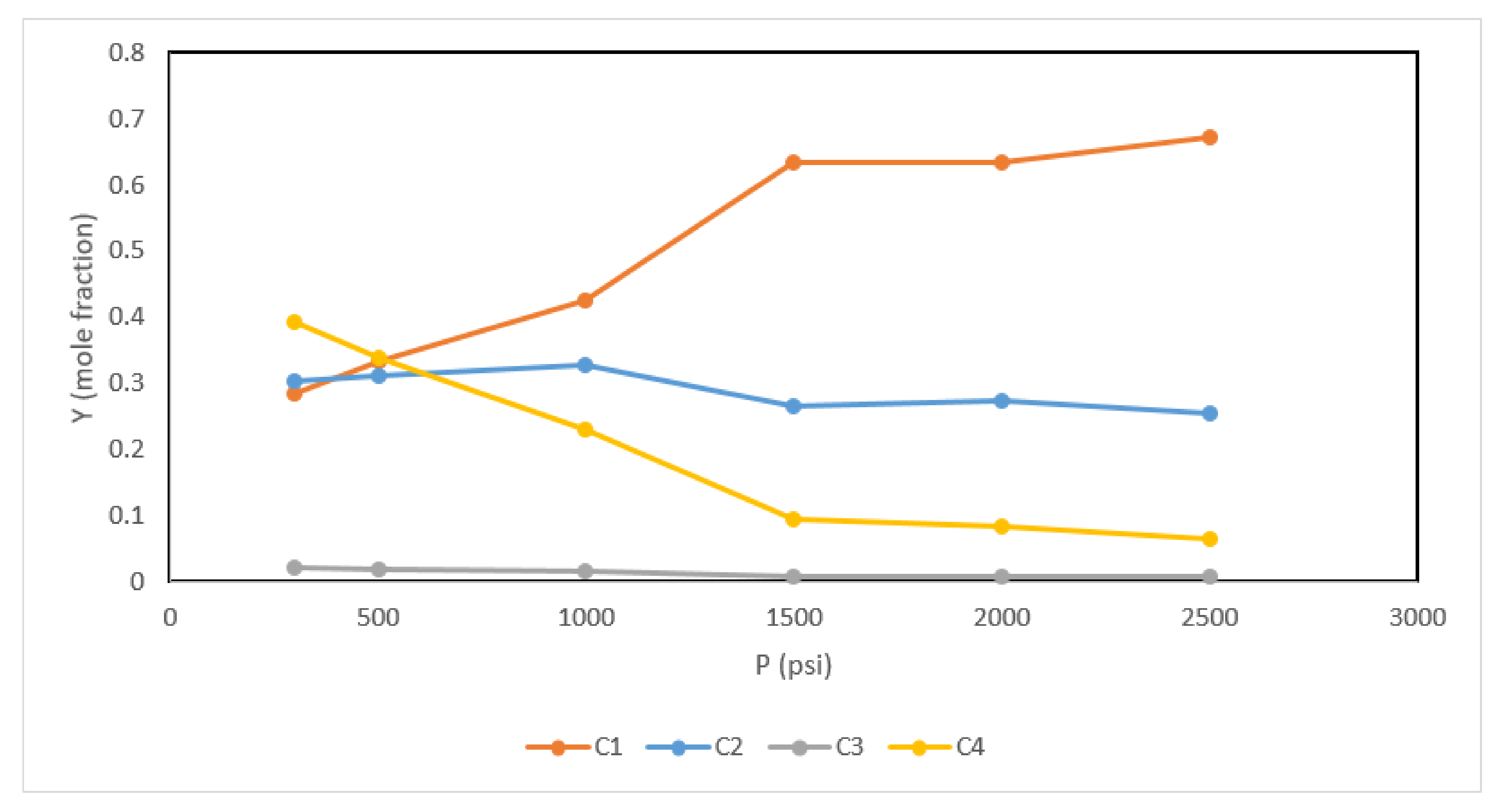
5. Results and Discussions

The nanoporous material was loaded with a mixture of C1-C4 at a pressure of 2500 psi and temperature equal to 194 °F (i.e., typical reservoir temperature). The bulk phase composition was arbitrary selected to be 0.3, 0.15, 0.2, and 0.35 for the four alkanes, respectively. The initial composition of the mixture was 0.673, 0.255, 0.0073, and 0.065, respectively, as shown in Table 1.
The sorption of the different components was obtained by using Grand Canonical ensemble [44]. The parameters of such ensemble are the adsorbed molecule chemical potential, volume, and temperature. The fugaicties were imposed for each component (i.e., its gas mixture with relative high pressure), which was the equivalent of using the chemical potential as follows:
μ i = μ i o + R T l n f i f i o
where μ i , μ i o ,   R , T ,   f i , and f i o are the chemical potential for component i, ideal chemical potential for component i, gas constant, temperature, fugacity of component i, and ideal fugacity of component i, respectively. All the adsorbent components were treated as rigid, except C1 due to the high fugacity value. Rigid type simplified the problem because there was no need to consider the solid–solid interaction energy [40].
The kerogen type II-D molecule shown in Figure 3 was recreated at the molecular platform and the nanoporous material was created by following the description provided in the previous section. Porosity was selected as 19.6% by adding 10 molecules of heptane during the construction phase and then deleting them afterwards. The initial composition of components in the nanoporous structure was obtained as shown in Table 2.
Desorption of hydrocarbons were carried out at a typical reservoir temperature of 194 °C and then at 284 °C. During the desorption stages, number of molecules of each component was monitored for further analysis. The total number of desorbed molecules for both cases is shown in Figure 4. The recovery factor RF is calculated as
R F = 1 n n i
where n is the total number of molecules present at a given depletion stage and ni is the initial number of molecules present at initial conditions. The ultimate recovery factor at the last desorption was 36%, whereas that of the heated case was almost 70%, indicating an improved recovery by two times.
The compositional variations at each pressure stage were obtained for typical reservoir and heated temperature cases, as shown in Figure 5 and Figure 6, respectively. For the typical temperature, the lightest component which was methane was selectively desorbed, leaving other heavier molecules behind. This behavior was referred to as the fractionation effect, where continuous compositional variations were observed. It can be seen from Figure 5 that gas composition is maintained constant above certain pressure, which is in this case was around 1500 psi (this pressure is called saturation pressure, which is the maximum adsorption capacity pressure). The structure above this pressure tended to hold on to its contained gases. However, the extent of that fractionation became more pronounced below saturation pressure (i.e., maximum adsorption capacity pressure). On the other hand, the fractionation effect was less severe for the heated case, as components maintained almost constant composition during desorption stages. The influence of compositional variations on the phase behavior was investigated by obtaining a P-T diagram for given composition of both cases at two stages of depletion, as shown in Figure 7 and Figure 8, respectively. It can be seen that the two-phase envelope was larger for the unheated case compared with the case of depletion at a higher temperature. The two-phase envelope of the unheated scenario continued to expand as kerogen pressure dropped further. This effect was attributed to the accumulation of heavier components. On the other hand, the two-phase envelope of the heat-assisted depletion almost stayed constant as all components were expelled from the structure uniformly. Hence, heating can reduce fractionation effect and potentially condensate problems to maximize the overall recovery.

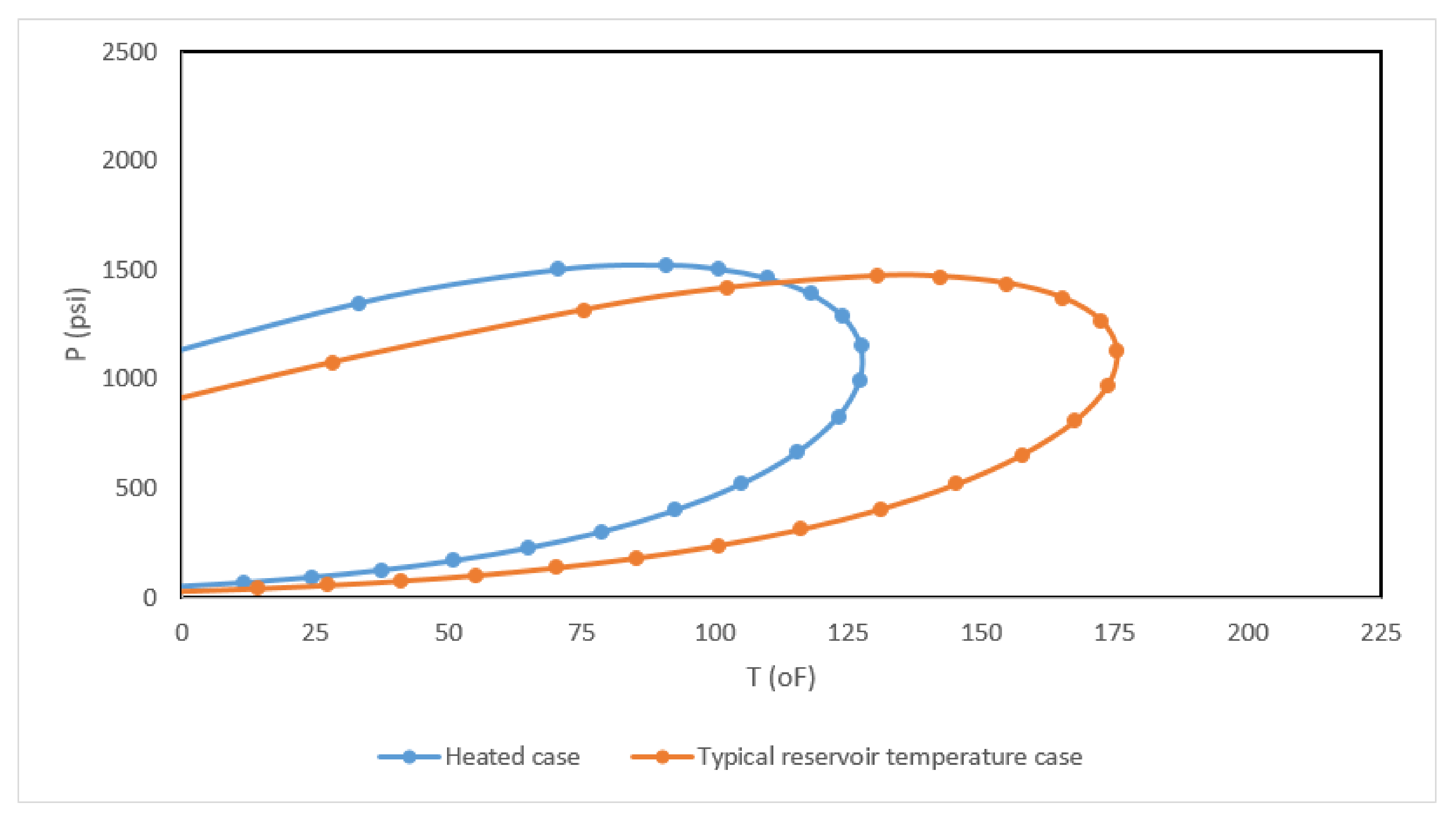
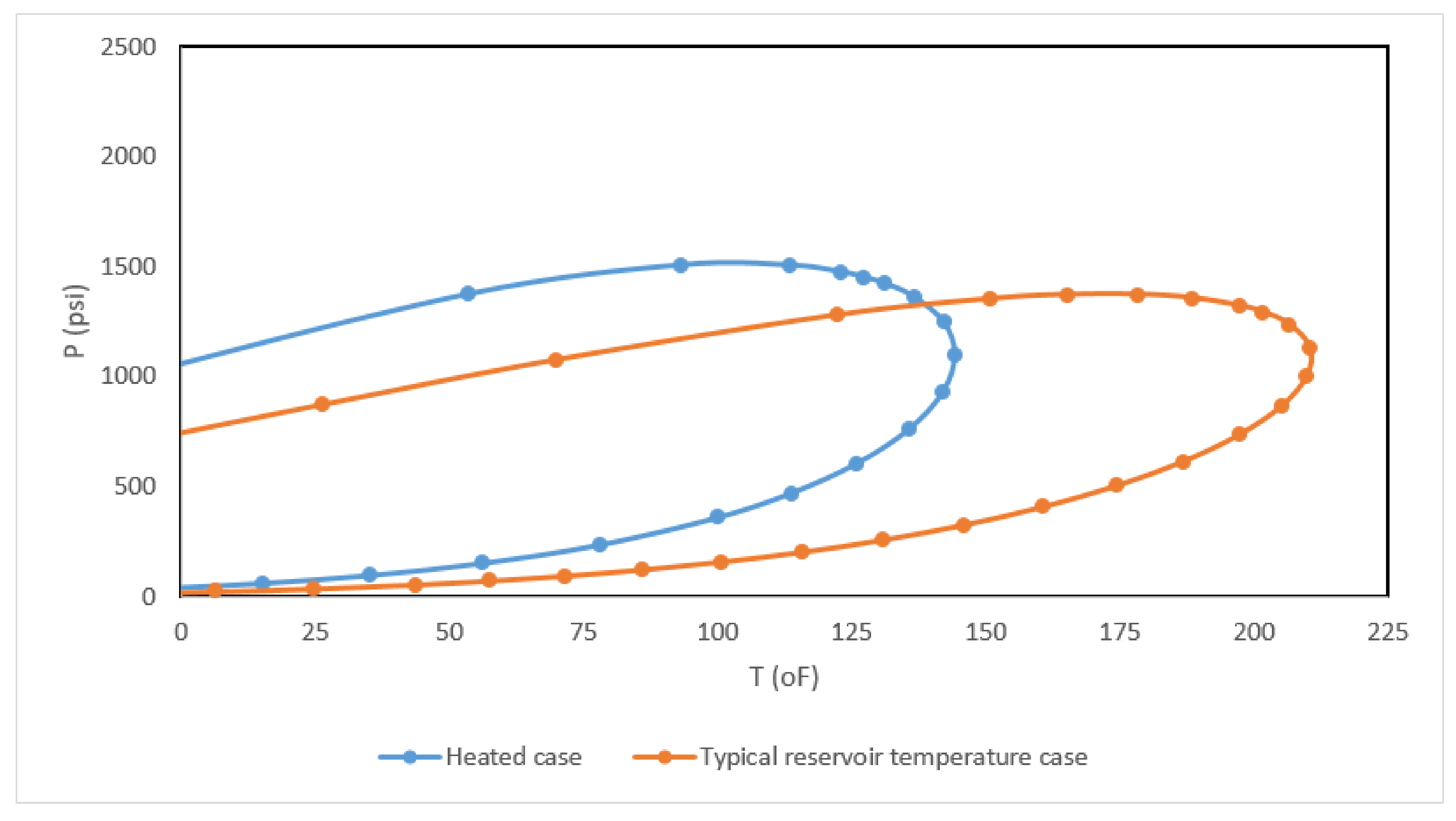
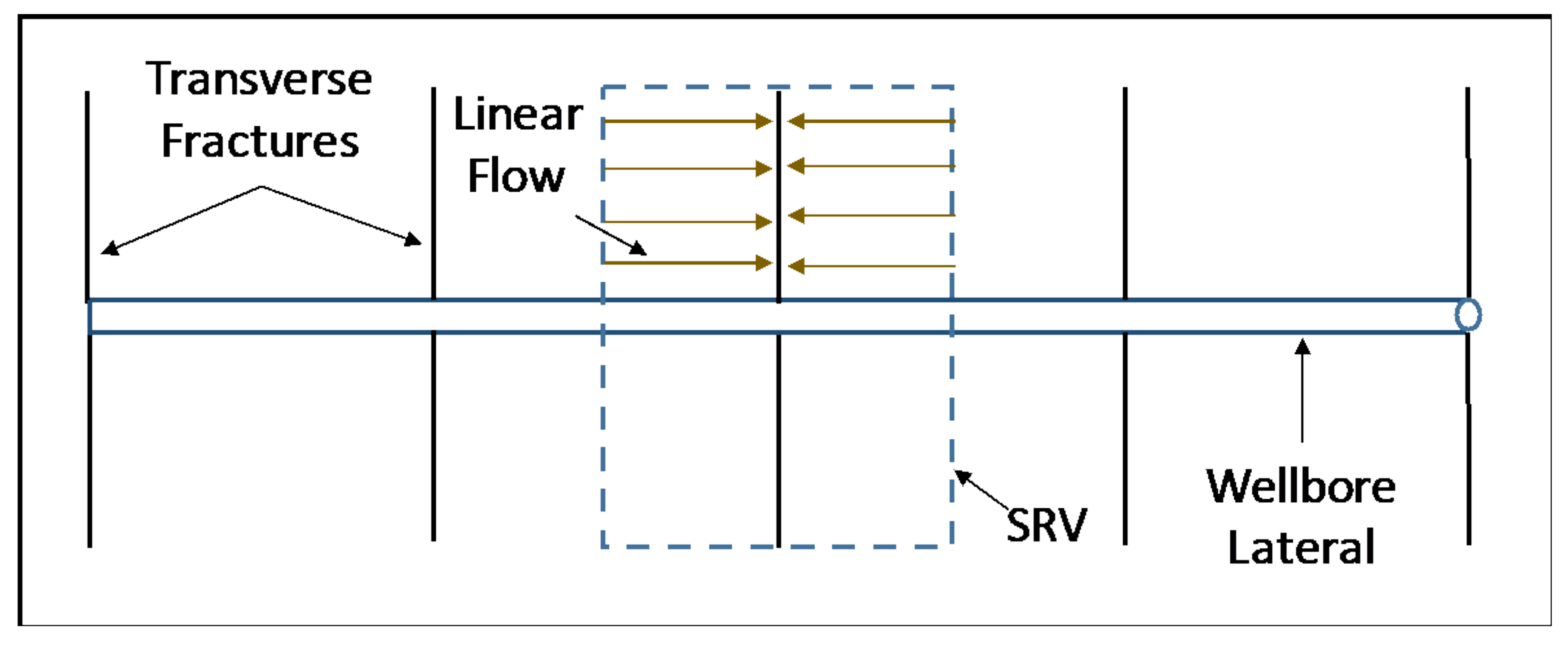
6. Reservoir Scale Heat Transfer Model

In this section, the feasibility of heating an unconventional reservoir by either injecting hot gas or by introducing a heating element was investigated. The model assumed transverse fractures intersecting the wellbore lateral created by multistage hydraulic fracturing (MSF), as shown in Figure 9. It also assumed that a 30 ft spacing between hydraulic fractures along a 4500 ft long lateral was designed, producing 150 transverse fractures. The fracture half-length was 400 ft, whereas the fracture height was 150 ft. Due to symmetry, the simulation domain was half of the stimulated reservoir volume (SRV), as shown in Figure 9.
A coupled heat and mass transfer model was used to study the heat propagation while injecting hot fluids. The detailed mathematical description is given in the Appendix A. The reservoir temperature was around 200 °F, whereas the gas was heated to 400 °F before injection. The thermal properties of the reservoir rock and fluids are shown in Table 3. The gas injector was simulated in this case to understand the heat propagation, given that the producer was neglected. It was found that the hot gas can advance heat to a sufficient distance only when a considerable amount was being injected for long periods. Figure 10 shows the heat propagation at a steady-state condition when injecting 0.5 MMscf/D and 1.0 MMscf/D of hot gas. The hydraulic fracture (one wing) was placed in the middle of the x-axis (0 location). As expected, most of the heating occurred within the fracture surroundings. Additionally, the larger the injection rate, the longer the heat penetration distance.
Hot gas injection was not feasible for many reasons. The process of gas injection is very expensive and could cause severe corrosion when CO2 is the selected gas. Additionally, the practice of heating gas while injecting and separating it after production is costly and unpractical. A considerable amount of gas must be injected; despite this, the heat does not fully propagate to the tip of the fracture. A large amount of heat could be lost around the wellbore, especially if it has to travel a long distance before reaching the perforation clusters. Figure 11 shows a comparison between the initial geothermal temperature and after injection temperature around the vertical wellbore section. Notice that the wellbore was placed on the west edge of the figure. As can be observed from the temperature magnitudes, a large amount of heat was lost to the formation before the hot fluids reached the fracture.
The other option would be placing a heated element around the lateral section of the wellbore. This would assume that the heated element was permanently placed at a constant temperature of 400 °F while the reservoir was under production (10 MMscf/D). The heating element was considered as a constant temperature boundary condition at the south side of the domain, as shown in Figure 12. The feasibility of the heated element arises from two facts: first, the heating propagation from the element into the reservoir does not act against the formation linear advection direction. Second, heat propagation, in this case, is transient and kept reaching new fronts as time progress (see Figure 12). As a matter of fact, heat propagation did not terminate while the heated element was operating. The mechanism at which the heat was propagated was through conduction within the formation's rock and fluids. In contrary to the previous scenario, the heat propagated almost equally through the SRV, except around the producing fractures. The reason was that the fluids were advected against the heat propagation only within the fracture.
Besides the heating time, two other factors can influence the heat propagation. First, the advection rate can significantly enhance heat transfer within the SRV, causing the heat to reach longer distances. Figure 13a shows the temperature map when the lateral was assumed to produce at 100 MMscf/D. The heat reached around 90 ft along the fracture direction, whereas only 55 ft for the 10 MMscf/D production case (see Figure 12b). Additionally, increasing the spacing between fractures can enhance heat propagation, as can be seen in Figure 13b. This is because an SRV will receive more heat flux, which improves the efficiency of heat transfer.

7. Conclusions

The common practice of producing unconventional resources through hydraulic fracturing can be enhanced when coupled with heating. The effect of temperature change on recovery was investigated for kerogen where significant amounts of hydrocarbons are stored. The computational work was carried out on a molecular replication of a kerogen sample using molecular simulations. The results showed an improved recovery by a factor of two with reduced fractionation effect in comparison with the non-heated case for the same applied pressure difference when the temperature was increased by 90 °F. Furthermore, the energy requirements to achieve that temperature rise at reservoir scale was investigated. Desired reservoir temperature for enhanced recovery could be achieved through resistive heating or fluid injection.

Author Contributions

Conceptualization, S.A. and M.A.; methodology, S.A.; software, R.W.; validation, G.G., S.A. and M.A.; formal analysis, S.A.; investigation, S.A.; resources, A.S.; data curation S.A.; writing—original draft preparation, S.A.; writing—review and editing, G.G.; supervision, A.S. All authors have read and agreed to the published version of the manuscript.

Funding

This research received no external funding.

Acknowledgments

Authors gratefully acknowledge College of Petroleum Engineering and Geoscience CPG support.

Conflicts of Interest

The authors declare no conflict of interest.

Nomenclature

P Pressure (psi)
T Temperature (°F)
Y Mole fraction (mole/mole)
f Fugacity (MPa)
C Specific heat capacity, kJ/(kg·°C)
k Thermal conductivity, kJ/(s·m·°C)
U Overall heat transfer coefficient, kJ/(s·m2·°C)

Appendix A

An integrated flow and heat transfer model was developed for a system containing a wellbore, fracture, and reservoir. These were integrated through the shared boundary conditions. The mathematical description of each model is shown below. Detailed description of the model was provided by Aljawad et al. [45].
The wellbore model is transient one-dimensional (1D), and projected to estimate the temperature of the fluid incoming to the fracture from the wellbore. The wellbore model is numerically coupled with a reservoir model to estimate the heat transfer from the wellbore to the surrounding formation. To obtain the velocity profile in the wellbore, the following continuity equation is solved:
ρ f t = 2 γ R w ρ f v L , p ρ f v z z
where t is injection time, R w is the wellbore radius, ρ f is the injected fluid density, γ is the wellbore open ratio, v L , p is the velocity of fluids entering the fracture, and z is the direction along the wellbore length. Obtaining the velocity profile makes it possible to solve the wellbore energy balance equation. The heat transfer equation within the wellbore can be written as
ρ f C ^ p f T w b t + v z T w b z + 2 γ R v L , p T w b T f B = 2 1 γ U R w T r B T w b
where T w b is the temperature of the wellbore, C ^ p f is the fluid’s specific heat capacity , T f B is the fracture temperature at the wellbore/fracture boundary, U   is the overall heat transfer coefficient between the wellbore and formation, and T r B is the temperature at the wellbore/formation (i.e., reservoir) boundary. The subscript B is used to represent the value at the boundary of the wellbore, reservoir, and fracture.
Solving Equation (A2) requires information about the fracture and formation temperatures. A procedure that requires iteration was implemented to solve the complete system. The geothermal temperature was considered as the initial condition. The radial reservoir heat conduction model was coupled along the wellbore, which can be written as
ρ C ^ p ¯ T r t = 1 r r r   k e ¯ T r r +   k e ¯ 2 T r   z 2
where ρ C ^ p ¯ is the average reservoir rock and fluid property, k e ¯ is the effective average thermal conductivity, and r is the radial direction away from the wellbore.
During injection, the fluid loss from the fracture induces fluid flow in the reservoir.
The flow in the coupled fracture/reservoir system can be estimated by solving diffusivity equation for compressible fluids, written as
· k n D m p = φ μ c t m p t
where k n D is the non-Darcy permeability, φ is the formation porosity, c t   is the total compressibility, and m(p) is the pseudo-pressure function.
That enables solving the heat transfer model in the reservoir/fracture system, which can be described as
ρ f C ^ p f T r t + φ β T T r p t + ρ f C ^ p f v · T r = · k f T r + β T T r 1 v · p
where β T is the thermal expansion factor, v is the velocity vector, k f is the fluid’s thermal conductivity vector, and p is the formation pressure. The first term in the above equation represents the accumulation of heat in the fracture, the second term is heat convection, and the last term is heat conduction.

References

  1. Ambrose, R.J.; Hartman, R.C.; Diaz-Campos, M.; Akkutlu, I.Y.; Sondergeld, C.H. Shale Gas-in-Place Calculations Part I: New Pore-Scale Considerations. SPE J. 2012, 17, 219–229. [Google Scholar] [CrossRef]
  2. Ertekin, T.; King, G.A.; Schwerer, F.C. Dynamic gas slippage: A unique dual-mechanism approach to the flow of gas in tight formations. SPE Form. Eval. 1986, 1, 43–52. [Google Scholar]
  3. Javadpour, F. Nanopores and Apparent Permeability of Gas Flow in Mudrocks (Shales and Siltstone). J. Can. Petrol. Technol. 2009, 48, 16–21. [Google Scholar] [CrossRef]
  4. Sakhaee-Pour, A.; Bryant, S. Gas Permeability of Shale. SPE Reserv. Eval. Eng. 2012, 15, 401–409. [Google Scholar] [CrossRef]
  5. Alafnan, S.F.K.; Akkutlu, I.Y. Matrix-Fracture Interactions during Flow in Organic Nanoporous Materials under Loading. Transp. Porous Med. 2018, 121, 69–92. [Google Scholar] [CrossRef]
  6. Alafnan, S. Pore Network Modeling Study of Gas Transport Temperature Dependency in Tight Formations. ACS Omega 4, 9778–9783. [CrossRef] [Green Version]
  7. Belyadi, H.; Fathi, E.; Belyadi, F. Hydraulic Fracturing in Unconventional Reservoirs: Theories, Operations, and Economic Analysis; Gulf Professional Publishing: Houston, TX, USA, 2019. [Google Scholar]
  8. Singh, H.; Javadpour, F. Langmuir slip-Langmuir sorption permeability model of shale. Fuel 2016, 164, 28–37. [Google Scholar] [CrossRef]
  9. Zhao, S.; Huang, W.W.; Wang, X.Q.; Fan, Y.R.; An, C.J. Sorption of Phenanthrene onto Diatomite under the Influences of Solution Chemistry: A Study of Linear Sorption based on Maximal Information Coefficient. J. Environ. Inform. 2019, 34, 33–54. [Google Scholar] [CrossRef]
  10. Yu, W.; Sepehrnoori, K. Numerical Model for Shale Gas and Tight Oil Simulation. In Shale Gas and Tight Oil Reservoir Simulation; Elsevier: Amsterdam, The Netherlands, 2018; pp. 11–70. [Google Scholar]
  11. Wang, X.; Wang, S.; Hagan, P.; Cao, C. Lacustrine Shale Gas: Case study from the Ordos Basin; Gulf Professional Publishing: Houston, TX, USA, 2017. [Google Scholar]
  12. Pini, R. Interpretation of net and excess adsorption isotherms in microporous adsorbents. Microporous Mesoporous Mater. 2014, 187, 40–52. [Google Scholar] [CrossRef]
  13. Menon, P.G. Adsorption at high pressures. Chem. Rev. 1968, 68, 277–294. [Google Scholar] [CrossRef] [Green Version]
  14. Zhou, Y.; Zhou, L. Fundamentals of high pressure adsorption. Langmuir 2009, 25, 13461–13466. [Google Scholar] [CrossRef] [PubMed]
  15. Kapoor, A.; Ritter, J.A.; Yang, R.T. An extended Langmuir model for adsorption of gas mixtures on heterogeneous surfaces. Langmuir 1990, 6, 660–664. [Google Scholar] [CrossRef]
  16. Do, D.D. Adsorption Analysis: Equilibria and Kinetics; Imperial College Press And Distributed By World Scientific Publishing Co: London, UK, 1998; Volume 2. [Google Scholar]
  17. Ruthven, D.M. Principles of Adsorption and Adsorption Processes; John Wiley & Sons: Hoboken, NJ, USA, 1984. [Google Scholar]
  18. Piñeiro, Á.; Brocos, P.; Amigo, A.; Gracia-Fadrique, J.; Lemus, M.G. Extended Langmuir Isotherm for Binary Liquid Mixtures. Langmuir 2001, 17, 4261–4266. [Google Scholar] [CrossRef]
  19. Van Assche, T.R.C.; Baron, G.V.; Denayer, J.F.M. An explicit multicomponent adsorption isotherm model: Accounting for the size-effect for components with Langmuir adsorption behavior. Adsorption 2018, 24, 517–530. [Google Scholar] [CrossRef]
  20. Michalec, L.; Lísal, M. Molecular simulation of shale gas adsorption onto overmature type II model kerogen with control microporosity. Mol. Phys. 2017, 115, 1086–1103. [Google Scholar] [CrossRef]
  21. Zhao, H.; Lai, Z.; Firoozabadi, A. Sorption Hysteresis of Light Hydrocarbons and Carbon Dioxide in Shale and Kerogen. Sci. Rep. 2017, 7, 1–10. [Google Scholar] [CrossRef] [Green Version]
  22. Hu, H. Methane adsorption comparison of different thermal maturity kerogens in shale gas system. Chin. J. Geochem. 2014, 33, 425–430. [Google Scholar] [CrossRef]
  23. Pang, Y.; He, Y.; Chen, S. An innovative method to characterize sorption-induced kerogen swelling in organic-rich shales. Fuel 2019, 254, 115629. [Google Scholar] [CrossRef]
  24. Fianu, J.; Gholinezhad, J.; Hassan, M. Comparison of Temperature-Dependent Gas Adsorption Models and Their Application to Shale Gas Reservoirs. Energy Fuels 2018, 32, 4763–4771. [Google Scholar] [CrossRef] [Green Version]
  25. Luo, S.; Nasrabadi, H.; Lutkenhaus, J.L. Effect of confinement on the bubble points of hydrocarbons in nanoporous media. AIChE J. 2016, 62, 1772–1780. [Google Scholar] [CrossRef]
  26. Walton, J.P.R.B.; Quirke, N. Capillary condensation: A molecular simulation study. Mol. Simulat. 1989, 2, 361–391. [Google Scholar] [CrossRef]
  27. Wongkoblap, A.; Do, D.D.; Birkett, G.; Nicholson, D. A critical assessment of capillary condensation and evaporation equations: A computer simulation study. J. Colloid Interface Sci. 2011, 356, 672–680. [Google Scholar] [CrossRef]
  28. Jiang, J.; Sandler, S.I. Capillary phase transitions of linear and branched alkanes in carbon nanotubes from molecular simulation. Langmuir 2006, 22, 7391–7399. [Google Scholar] [CrossRef]
  29. Singh, S.K.; Sinha, A.; Deo, G.; Singh, J.K. Vapor-Liquid Phase Coexistence, Critical Properties, and Surface Tension of Confined Alkanes. J. Phys. Chem. C 2009, 113, 7170–7180. [Google Scholar] [CrossRef]
  30. Didar, B.R.; Akkutlu, I.Y. Pore-Size Dependence of Fluid Phase Behavior and Properties in Organic-Rich Shale Reservoirs. In Proceedings of the SPE International Symposium on Oilfield Chemistry, The Woodlands, TX, USA, 8–10 April 2013. [Google Scholar] [CrossRef]
  31. Pitakbunkate, T.; Balbuena, P.B.; Moridis, G.J.; Blasingame, T.A. Effect of confinement on pressure/volume/temperature properties of hydrocarbons in shale reservoirs. SPE J. 2016, 21, 621–634. [Google Scholar] [CrossRef]
  32. Bui, K.; Akkutlu, I.Y. Hydrocarbons Recovery from Model-Kerogen Nanopores. Soc. Petrol. Engs. 2017, 22, 854–862. [Google Scholar] [CrossRef]
  33. Curtis, E.M. Influence of thermal maturity on organic shale microstructure. (n.d.). Available online: http://www.ogs.ou.edu/MEETINGS/Presentations/2013Shale/2013ShaleCurtis.pdf (accessed on 9 March 2019).
  34. Chen, S.; Han, Y.; Fu, C.; Zhang, H.; Zhu, Y.; Zuo, Z. Micro and nano-size pores of clay minerals in shale reservoirs: Implication for the accumulation of shale gas. Sediment. Geol. 2016, 342, 180–190. [Google Scholar] [CrossRef]
  35. Hou, Y.; He, S.; Wang, J.; Harris, N.B.; Cheng, C.; Li, Y.; Pedersen, P. Preliminary study on the pore characterization of lacustrine shale reservoirs using low pressure nitrogen adsorption and field emission scanning electron microscopy methods: A case study of the Upper Jurassic Emuerhe Formation, Mohe basin, northeastern China. Can. J. Earth Sci. 2015, 52, 294–306. [Google Scholar]
  36. Wasaki, A.; Akkutlu, I.Y. Permeability of organic-rich shale. SPE J. 2015, 20, 381–384. [Google Scholar] [CrossRef]
  37. Kou, R.; Alafnan, S.F.K.; Akkutlu, I.Y. Multi-scale Analysis of Gas Transport Mechanisms in Kerogen. Tranp. Porous Med. 2017, 116, 493–519. [Google Scholar] [CrossRef]
  38. Ungerer, P.; Collell, J.; Yiannourakou, M. Molecular modeling of the volumetric and thermodynamic properties of kerogen: Influence of organic type and maturity. Energy Fuels 2015, 29, 91–105. [Google Scholar] [CrossRef]
  39. Plimpton, S. Fast Parallel Algorithms for Short-Range Molecular Dynamics. J. Comput. Phys. 1995, 117, 1–19. [Google Scholar] [CrossRef] [Green Version]
  40. Yiannourakou, M.; Ungerer, P.; Leblanc, B.; Rozanska, X.; Saxe, P.; Vidal-Gilbert, S.; Gouth, F.; Montel, F. Molecular simulation of adsorption in microporous materials. Oil Gas Sci. Technol. 2013, 68, 977–994. [Google Scholar] [CrossRef] [Green Version]
  41. Hoover, W.G. Canonical dynamics: Equilibrium phase-space distributions. Phys. Rev. A 1985, 31, 1695–1697. [Google Scholar] [CrossRef] [PubMed] [Green Version]
  42. Zhang, T.; Ellis, G.S.; Ruppel, S.C.; Milliken, K.; Yang, R. Effect of organic-matter type and thermal maturity on methane adsorption in shale-gas systems. Org. Geochem. 2012, 34, 120–131. [Google Scholar] [CrossRef]
  43. Tian, Y.; Yan, C.; Jin, Z. Characterization of Methane Excess and Absolute Adsorption in Various Clay Nanopores from Molecular Simulation. Sci. Rep. 2017, 7, 1–21. [Google Scholar] [CrossRef] [Green Version]
  44. Nicholson, D.; Parsonage, N.G. Computer Simulation and the Statistical Mechanics Ofadsorption; Academic Press: New York, NY, USA, 1982. [Google Scholar]
  45. Aljawad, M.S.; Alafnan, S.; Abu-Khamsin, S. Artificial Lift and Mobility Enhancement of Heavy Oil Reservoirs Utilizing a Renewable Energy-Powered Heating Element. ACS Omega 2019, 4, 20048–20058. [Google Scholar] [CrossRef] [Green Version]
Figure 1. Conceptual model to study multicomponent hydrocarbons transport in organic material microcrack system.
Sustainability 12 02145 g001
Figure 2. Kerogen type II-D as created by Ungerer et al. (2015).
Sustainability 12 02145 g002
Figure 3. NVT/NPT simulation parameters.
Sustainability 12 02145 g003
Figure 4. Adsorption as a function of pressure at typical reservoir temperature and at elevated temperature.
Sustainability 12 02145 g004
Figure 5. Compositional variation for desorption stages at typical reservoir temperature of 194 °F.
Sustainability 12 02145 g005
Figure 6. Compositional variation for desorption stages at elevated reservoir temperature of 284 °F.
Sustainability 12 02145 g006
Figure 7. P-T diagram generated at the gas composition of typical (orange) and heated (blue) when the kerogen pressure dropped to 1000 psi. The typical reservoir temperature had a larger two-phase envelope due to accumulation of heavier components.
Sustainability 12 02145 g007
Figure 8. P-T diagram generated at the gas composition of typical (orange) and heated (blue) when the kerogen pressure dropped to 500 psi. The two-phase envelope continued to increase for the typical reservoir temperature while maintaining its shape for the heated case.
Sustainability 12 02145 g008
Figure 9. Schematic of multistage hydraulic fracturing and stimulated reservoir volume (SRV).
Sustainability 12 02145 g009
Figure 10. Heat propagation within the SRV when a hot fluid was injected at two different injection rates. (a) Heat propagation at 0.5 MMscf/D and (b) at 1.0 MMscf/D.
Sustainability 12 02145 g010
Figure 11. (a) Initial formation geothermal temperature. (b) Formation temperature around the vertical wellbore section after hot fluids injection.
Sustainability 12 02145 g011
Figure 12. Heat propagation within the SRV when placing a heating element (south side of the figure) at different heating times. Mapping of heat propagation is shown after (a) 3 months and (b) 3 years.
Sustainability 12 02145 g012
Figure 13. Heat propagation within the SRV when placing a heating element at (a) high production rate (100 MMscf/D), and at (b) lower production rate (10 MMscf/D) but with larger fracture spacing.
Sustainability 12 02145 g013
Table 1. Bulk phase composition to load kerogen with molecules.
ComponentCompositionFugacity (psi)
CH430%1061.1
C2H615%195.7
C3H820%123.4
n-C4H1035%106.2
Table 2. Initial composition of the loaded kerogen at 2500 psi.
CH4C2H6C3H8n-C4H10
67.30%25.50%0.73%6.50%
Table 3. Thermal properties of the reservoir fock and fluids.
Input DataSI UnitField Unit
Ambient temperature, T b 25 °C77 °F
Reservoir temperature, T R 93.33 °C200 °F
Gas temperature at injection or element temperature, T I 204.4 °C400 °F
Formation specific heat capacity, c m a 0.879 kJ/(Kg·°C)0.2099 Btu(lb·°F)
Formation thermal conductivity, k m a 1.57 × 10⁻³ kJ/(s·m·°C)0.907 Btu/(hr·ft·°F)
Gas heat capacity,   c p 2.18 kJ/(Kg·°C)0.52 Btu/(lbm·°F)
Gas thermal conductivity,   k 5.5 × 10⁻⁵ kJ/(s·m·°C)0.0318 Btu/(hr·ft·°F)
Overall heat transfer coefficient, U 0.1 kJ/(s·m2·°C)0.00488 Btu/(hr·ft2·°F)

